Statistical Validation Framework for Automotive Vehicle Simulations Using Uncertainty Learning

Abstract

The modelling and simulation process in the automotive domain is transforming. Increasing system complexity and variant diversity, especially in new electric powertrain systems, lead to complex, modular simulations that depend on virtual vehicle development, testing and approval. Consequently, the emerging key requirements for automotive validation involve a precise reliability quantification across a large application domain. Validation is unable to meet these requirements because its results provide little information, uncertainties are neglected, the model reliability cannot be easily extrapolated and the resulting application domain is small. In order to address these insufficiencies, this paper develops a statistical validation framework for dynamic systems with changing parameter configurations, thus enabling a flexible validation of complex total vehicle simulations including powertrain modelling. It uses non-deterministic models to consider input uncertainties, applies uncertainty learning to predict inherent model uncertainties and enables precise reliability quantification of arbitrary system parameter configurations to form a large application domain. The paper explains the framework with real-world data from a prototype electric vehicle on a dynamometer, validates it with additional tests and compares it to conventional validation methods. It is published as an open-source document. With the validation information from the framework and the knowledge deduced from the real-world problem, the paper solves its key requirements and offers recommendations on how to efficiently revise models with the framework’s validation results.

1. Introduction

The automotive development process is both highly complex and is becoming more diverse thanks to increasing possibilities in modelling, computing and analysing, especially in the field of new electric powertrain systems [1,2,3]. The early stages of the process offer a great deal of freedom when the development comes to realising the vehicle specifications [4]. In order to compare the different options, evaluating as many properties of the final product as possible [5] is important. As today’s research and development work increasingly depends on predictions based on system simulations [6], their reliability quantification is essential for creating new knowledge, the transparent evaluation of options for action and to support safety-relevant decisions based on simulation results [7].

The modelling and simulation (M+S) process and analysis methods used in automotive development are undergoing a transformation and new requirements are emerging. An increasing system complexity and growing variant diversity lead to more complex and modular simulation models. This transformation needs virtual vehicle development, testing and approval in a large application domain [1,8]. Better knowledge of systems, such as the ability to precisely quantify uncertain parameters, is needed to ensure a more accurate understanding of systems that affect the safety and efficiency of complex powertrains [9,10] and non-linear dynamic systems [11,12,13]. As described in Danquah et al. [1], the new key requirements of validation include a more precise reliability quantification of simulation results in a large application domain, achieved at reasonable cost and time. What is meant by large application domain is a precise evaluation of the simulation’s output reliability under changing system parameters, system scenarios or system topologies. Part of the information can be obtained from existing verification and validation (V+V) processes. Nonetheless, the information is not enough to fulfil the new requirements, because their validation provides scant information on the reliability of the simulation results [14,15,16]. Danquah et al. [1] identified four key insufficiencies that prevent conventional validation methods from meeting the new requirements:

1.

the negligence of uncertainty,

2.

the binary, low-information validation result,

3.

the low extrapolation capability of model reliability,

4.

the small application domain size.

This paper addresses those insufficiencies by developing a statistical verification, validation and uncertainty quantification (VV+UQ) framework. The framework focuses on dynamic systems with changing parameter configurations, thus enabling a flexible validation of complex total vehicle simulations including powertrain and consumption modelling. It uses non-deterministic models to include input uncertainties, applies uncertainty learning to predict inherent model uncertainties and thus enables the precise reliability quantification of arbitrary system parameter configurations to form a large application domain. The main contributions are:

• Summarising the insufficiencies of validation in the automotive domain, which prevent a reliability assessment of simulation models and system safety.
• A statistical VV+UQ framework with uncertainty learning for the precise validation of a large application domain.
• First application of a statistical VV+UQ framework predicting model uncertainties of new parameter configurations.
• Explanation, validation and discussion of the framework with real world data from a prototype electric vehicle on a roller dynamometer.
• Solving the new key requirements of automotive validation and recommending four improvement strategies to allow efficient error targeting for revising automotive M+S processes and total system understanding.

After defining validation and summarizing the problems in Section 2, the basic VV+UQ framework and the test system setup are explained in Section 3 and Section 4. In Section 5, the validation framework validates a modular longitudinal simulation model. Section 6 applies the model in a large application domain using uncertainty learning to predict the model reliability. Real data were collected from statistical consumption measurements for an electric vehicle on a roller dynamometer for this purpose. After validating the framework with additional test data in Section 7, Section 8 concludes the most important research findings.

2. Model Validation

This section explains the foundations of V+V and identifies the problems in automotive validation that will be addressed in the statistical validation framework in the next sections. Section 2.1 is a compact summary of ([1], Section 2.1), Section 2.2 is a summary of ([1], Section 2.2) and Section 2.3 is a summary of ([1], Sections 3.4 and 4.2) and ([4], Section 2.2).

2.1. Philosophy of the Science of Validation

So as to be able to improve V+V, the paper begins by clarifying the philosophical foundations of validation theory and its terminology. Kleindorfer et al. [17] come to the conclusion that the problem of correct validation is an ethical issue, whereby the warranty offered by the model and evidence around the model must be carefully justified. Popper [18,19] introduces the theory of falsificationism. Since natural systems are never self-contained, he and Oreskes et al. [20] agree that they are impossible to validate. Theories can be confirmed by observations, but due to the limited access to natural phenomena, there is never proof of their complete accuracy. The discussion of V+V has converged in some communities ([21], p. 21). Thus, the IEEE [22] states that V+V is accepted when the model meets defined specifications. This definition is incorporated into ISO 9000 [23]. The American Society of Mechanical Engineers (ASME) Guide [24] accepts the validation definition of the US Department of Defence [25] and defines verification as:

Verification: The process of determining that a computational model accurately represents the underlying mathematical model and its solution.

Validation: The process of determining the degree to which a model is an accurate representation of the real world from the perspective of the intended uses of the model.

For the purpose of this paper, the theory or entity is characterised by a simulation model. According to the definition of Neelamkavil [26], a model is a representation of a real system and simulation is the mimicking of model behaviour. This means that for a valid, correct use of the model, the reliability of its results must be determined individually for each application. The conclusion from the philosophy of science is that it is almost impossible to validate a model that aims to reflect reality.

2.2. Validation Processes

There are widely accepted V+V processes to validate the M+S process. They focus on practical approaches and less on the truth in the philosophy of science [21]. As shown in Figure 1, Sargent [27] developed a V+V process and defined operational validity as the determination of whether the output behaviour of the model has a satisfactory range of precision for its intended purpose within the area of intended applicability. The V+V process of Sargent is similar to the approaches of Oberkampf and Trucano [28] and the ASME Guide [24]. This V+V process is one of the most broadly acknowledged in the validation of M+S [16] and will be referred to as the conventional process in this paper.

Because conventional validation is strongly oriented towards its practicability, statistical validation methods are emerging that cover a better fulfilment of truth in the philosophy of science, while maintaining the necessary practicability in engineering [21]. Statistical validation assumes a natural true value $y_{\mathrm{nature}}$ of a real system’s or entity’s output response quantity of interest (SRQ). This value is often called ground truth or true value [30]. When the output value $y_{\mathrm{s}}$ of the system $G_{\mathrm{s}}$

$$G_{\mathrm{s}}:\left(x,\theta \right)\mapsto y_{\mathrm{s}}$$

(1)

$$G_{\mathrm{m}}:\left(x,\theta \right)\mapsto y_{\mathrm{m}}$$

(2)

is measured, there will always be an error $e_{y_{\mathrm{s}},\mathrm{obs}}$ between observation and true value. The simulation model $G_{\mathrm{m}}$ estimates the true value of the nature of the SRQ based on the input of time-variant signals x and the time-invariant parameters $\theta$ through its output value $y_{\mathrm{m}}$ (2). The errors e indicate the discrepancy between the simulated and true value. They are inherent in every simulation model because a model is by definition a simplified abstraction of reality [26]. One source of errors results from the calculation of finite accuracy by computers compared to the exact solution of the mathematical model $e_{\mathrm{h}}$. A further source of error results from the model time-variant inputs $e_{\mathrm{x}}$ and the time-invariant parameters $e_{\theta }$. Whereas they are usually assumed to be fully characterized in a conventional validation of deterministic simulations, these errors are mostly unknown in reality. Moreover, the model itself contains model form errors $e_{\mathrm{m}}$ due to the selection of an unsuitable equation. They can be quantified based on physical data from model validation experiments. Therefore, the experimental results of the physical system $G_{\mathrm{s}}$ and the simulation results of the model $G_{\mathrm{m}}$ are compared using validation metrics [31]. As defined in ASME [32], the involved errors can be summarized as:

$$y_{\mathrm{nature}}=G_{\mathrm{s}}\left(x,\theta \right)-e_{y_{\mathrm{s}},\mathrm{obs}}$$

(3)

$$y_{\mathrm{nature}}=G_{\mathrm{m}}\left(x,\theta ,h\right)-(e_{\mathrm{m}}+e_{\mathrm{x}}+e_{\theta }+e_{\mathrm{h}})$$

(4)

The basic theory behind statistical methods states that because those errors cannot be exactly estimated, they need to be approximated through uncertainties, which are expressed in probability functions or confidence intervals [33]. The various sources of uncertainty are deeply interwoven and affect each other. Depending on the constellation, they may reinforce or compensate each other, which can result in a misleading trustworthiness of the simulation model ([21], p. 385). It is therefore helpful to quantify the different uncertainties separately. Additional sources such as observation errors $e_{y,\mathrm{obs}}$ or extrapolation errors caused by model predictions beyond the validity range make this even more difficult. As explained in Figure 2, the uncertainties can be point valued, if accurately known, epistemic, resulting in an interval, aleatory, resulting in a cumulative distribution function (CDF), or mixed, resulting in a probability box (p-box). It should be noted that the definition of Oberkampf and Roy [21] for epistemic uncertainties is used, which treats purely epistemic uncertainties as an interval-valued quantity with no likelihood information specified. This assumption should not be confused with definitions in other disciplines, where epistemic uncertainties can contain subjective probability distributions [34].

In deterministic simulations, the errors and uncertainties are usually assumed to be fully characterised. This is not the case for partially and uncharacterised experiments as well as unknown model prediction conditions [35]. Therefore, non-deterministic simulations aggregate these uncertainties through the model to the result side for statistical validation. The most important framework that uses statistical validation is the VV+UQ framework of Oberkampf and Roy [21]. This uses a probability bound analysis, which was greatly influenced by Ferson et al. [36]. It clearly distinguishes between the input, numerical and model form and prediction uncertainties to improve the validation of CFD simulations. Sankararaman and Mahadevan [37] use a Bayesian network to aggregate all types of uncertainties in general engineering simulations. It has the advantage that heterogeneous information on several levels of the system architecture can be combined to a total prediction uncertainty.

2.3. Statistical Validation in Automotive Domain

The review of Danquah et al. [1] analyses more than 30 validation frameworks in the automotive domain from 1990 to 2020. It concludes that the analysed frameworks agree with the validation concept of Sargent. Since validation in the automotive domain only uses conventional tolerance-based metrics, four key insufficiencies arise:

The negligence of uncertainty: Conventional validation assumes that the data utilised in the process are valid. In practice, the data used for validation are not fully known, or may even be completely unknown. It is the law of nature that there will be a discrepancy. If valid input and output data, parameters and boundary conditions are assumed, errors are neglected. These uncertainties are underestimated and may become uncontrollably large when they accumulate ([21], p. 385).

Binary, low-information validation result: The conventional validation is binary ([38], p. 6). A model can be valid or invalid. This can never be proven to be true, because the philosophy of science tells us that absolute evidence is impossible. Validation should ask the question of the intended purpose and consider the degree of correctness [28,37].

Extrapolation capability of model reliability: Since an extrapolation of validity is not anticipated in conventional validation, almost no knowledge of the M+S process is gained beforehand, which makes extrapolation almost impossible. Conclusions outside the scope of the measured validation range are mere suppositions [14]. Conventional validation must re-validate the model if the conditions or the use case changes.

Application domain size: As validation is time-consuming and expensive, a simulation model can often only be validated by measurements of a few points. Since conventional validation does not foresee extrapolation, the application domain is restricted to the validation measurements. To close this gap, statistical validation allows extrapolation when information about the uncertainty of former validations is accessible [39].

Those four insufficiencies prevent validation from meeting the new key requirements. As analysed in Danquah et al. [1], there are attempts to address these problems by integrating statistical methods. They conclude that the problem has not been solved because the analysed authors did not consistently integrate statistical approaches. To meet the new key requirements, Danquah et al. [1] propose a consistent statistical validation method, which has a high potential to solve those four key insufficiencies [1,4].

3. Statistical Validation Method

This paper develops a statistical VV+UQ framework for dynamic systems with changing parameter configurations that enables a flexible statistical validation for complex total vehicle simulations. The key requirements are precise reliability quantification in a large application domain at a reasonable cost and time.

3.1. Concept and Previous Work

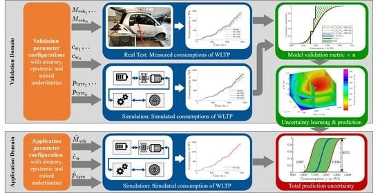
This framework takes its fundamental ideas from the statistical VV+UQ frameworks of Oberkampf and Roy [28,40] and Mahadevan and Sankararaman [37,41]. While Oberkampf [21] specialises in computational fluid dynamics and Mahadevan [41] in general engineering systems, this framework focuses on multi-component, modular models with a large number of parameters in automotive total vehicle simulations. Previous work has been carried out in the automotive domain, upon which this framework is directly based: (1) the review of Danquah et al. [1], which analyses and structures statistical validation frameworks. (2) The review of Riedmaier et al. [30], which compares a large number of uncertainty validation frameworks and brings them into one main structure. (3) The method and application of Danquah et al. [4], which is concentrated on statistical validation metrics for automotive total vehicle simulation. The statistical validation application with theoretical data of Riedmaier et al. [42] focuses on predicting the reliability quantification of simulation results under new application scenarios of autonomous vehicles. In contrast, this paper focuses on predicting the reliability quantification of simulation results under new application parameter configurations using real experimental data. In this paper, parameter configurations are internal vehicle parameters and not external scenarios or scenario parameters. The basic idea of the validation framework is explained in Figure 3.

In M+S, it is essential to validate and estimate the reliability of a model and each single simulation result depending on arbitrary parameter configurations of a large application domain a. Therefore, the model and result reliability of several validation parameter configurations must be estimated with multiple validation experiments forming the validation domain v. The model and result reliability in the application domain can be predicted through inter- and extrapolation based on the knowledge about the reliability from the validation domain.

3.2. Detailed Explanation

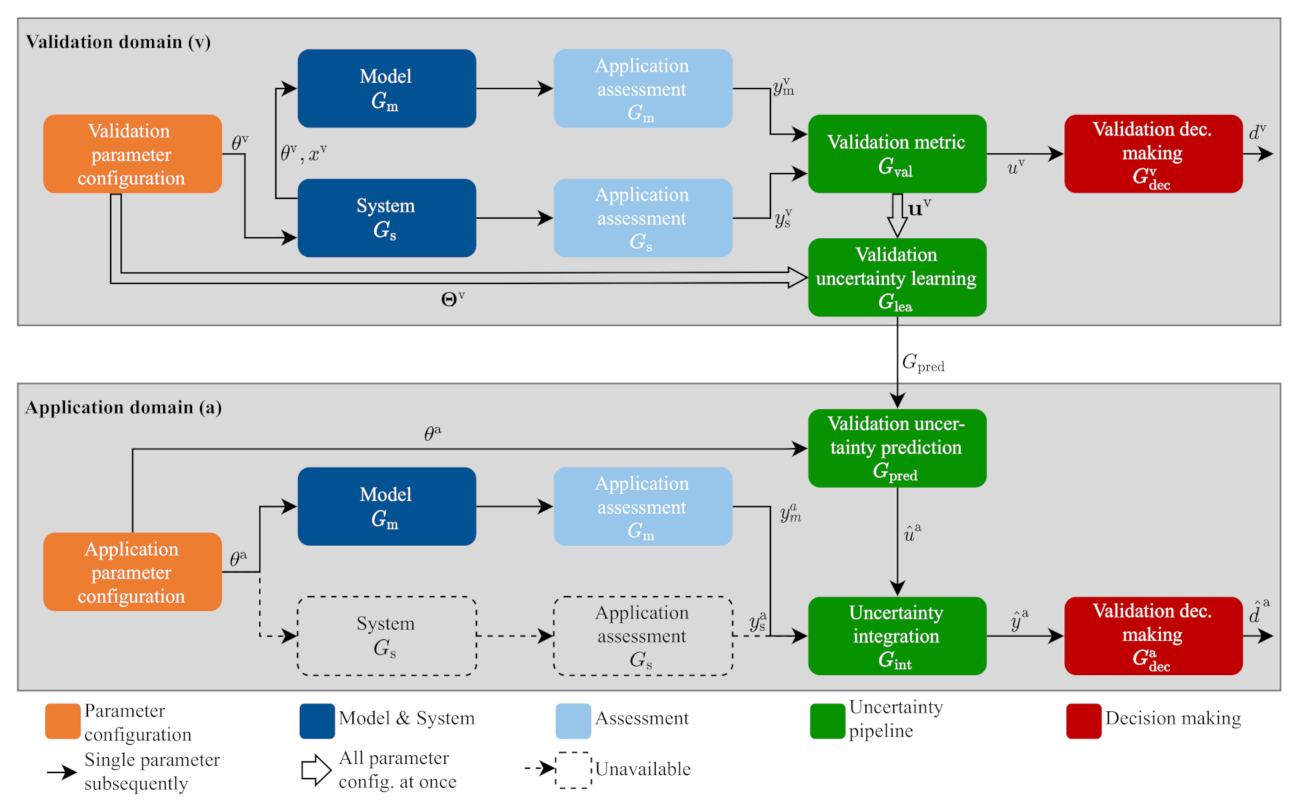
The validation framework is explained in detail in Figure 4. The aim is to give an overview of the framework and to introduce symbols and the nomenclature. The framework considers a model $G_{\mathrm{m}}$ shown in Equation (2). Based on the input of time-variant signals x and the time-invariant parameters $\theta$, the simulation of the model mimics the behaviour of the system $G_{\mathrm{s}}$ to approximate the system output SRQ $y_{\mathrm{s}}$. The simulation result $y_{\mathrm{m}}$ is an estimate of the measured SRQ $y_{\mathrm{s}}$. As shown in Figure 2, all inputs and outputs of a model can be single-value, aleatory, epistemic or mixed. Before starting with the actions in Figure 4, the model must be verified and the model inputs and their uncertainties quantified. For detailed information on how to estimate and calibrate uncertain parameters, please refer to the four publications [1,4,30,43]. In the validation domain, the results of a real system $y_{\mathrm{s}}^{\mathrm{v}}$ measured during a fixed validation parameter configuration ${\theta }^{\mathrm{v}}$ are compared to the results of the model $y_{\mathrm{m}}^{\mathrm{v}}$. A validation metric $G_{\mathrm{val}}$ compares both results to get an estimate of the model error, which leads to the model uncertainty $u^{\mathrm{v}}$. A non-deterministic model is needed to consider the uncertain model inputs. To cover the validation domain, several validation parameter configurations concluded in the validation configurations ${\mathsf{\Theta }}^{\mathrm{v}}$ must be validated by estimating the corresponding model uncertainties concluded in ${\mathit{u}}^{\mathrm{v}}$. These tests are needed to enable validation uncertainty learning $G_{\mathrm{lea}}$. The result reliabilities of new application parameter configurations ${\theta }^{\mathrm{a}}$ are estimated in the application domain. This process can be called the validation of an application parameter configuration. Because no system is available to provide real measurements $y_{\mathrm{s}}^{\mathrm{a}}$, it is necessary to validate the result by approximating the model uncertainty ${\widehat{u}}^{\mathrm{a}}$ through the validation uncertainty prediction $G_{\mathrm{pred}}$. This uses the data from uncertainty learning $G_{\mathrm{lea}}$ to inter- or extrapolate to the model uncertainty ${\widehat{u}}^{\mathrm{va}}$ of the current application parameter configuration ${\theta }^{\mathrm{a}}$. The approximated model uncertainty ${\widehat{u}}^{\mathrm{a}}$ and the simulation result of the application configuration $y_{\mathrm{m}}^{\mathrm{a}}$ need to be integrated with the integration model $G_{\mathrm{int}}$ to calculate the total prediction uncertainty ${\widehat{y}}^{\mathrm{a}}$. An application decision-making $G_{\mathrm{dec}}^{\mathrm{a}}$ decides if the result of the total prediction uncertainty is accurate enough for the intended use case. The basic structure of the framework shown in Figure 4 stays the same. There are several possibilities to conduct the individual steps of the framework that are interchangeable, which leads to some modularity. Several variants, combinations and advantages of them are explained in the review of Riedmaier et al. [30]. One variant with all steps will be explained and validated in detail with real data in this paper.

4. System, Model and Parameters

This section explains the framework in detail with a real-world example. For this purpose, a dataset is measured and published as an open-source document along with this paper [44]. The example test setup, the verification of the model and parameter identification are explained in this section.

4.1. System Setup, Control and Measurement

The example validates a total vehicle simulation with a focus on longitudinal dynamics and consumption. A detailed powertrain model is used to calculate the dynamics of the vehicle, which is necessary for the precise calculation of the energy consumption. The model calculates the consumption of the Worldwide Harmonised Light Vehicle Test Procedure (WLTP) Class 2 cycle of the prototype vehicle called NEmo. For the validation, a real system test is executed, where the vehicle is put on a roller dynamometer. For the precise evaluation of the dynamics and the consumption, additional sensors are integrated in the vehicles powertrain. The physical system setup is shown in Figure 5 and the schematic setup with the components, sensors, controls and data logging in Figure 6.

NEmo is a modified Smart with a prototype powertrain developed in Wacker et al. [45]. It has the advantages of integrated multiple sensors, a programmable power electronics and a programmable vehicle control unit. The target torque of the motor $T_{\mathrm{target},\mathrm{mot}}$ and the wheel brakes $T_{\mathrm{target},\mathrm{wheel}}$ can be set and the speed of the axis $\dot{\omega }$ can be measured via controller area network (CAN). This enables accurate and repeatable speed control. A battery simulator serves as power supply, where the voltage U can be controlled via CAN. The roller dynamometer imprints the vehicle longitudinal driving forces $F_{\mathrm{dyna}}$ depending on the actual vehicle acceleration and speed. Using this system setup, the environment can be controlled and all tests are repeatable and comparable. Additionally, vehicle parameters like mass, roll resistance and air resistance can be physically changed to measure multiple validation parameter configurations. This is essential for statistical validation uncertainty learning and prediction.

4.2. Simulation Model and Verification

The simulation model used is re-parametrised based on the already published model, in which the simulation results are verified with real data by Danquah et al. [46]. It can be downloaded with an open-source license in Danquah et al. [47]. Since this model is open source, it is very popular with several independent researchers [48,49,50,51] and has been improved over the last years by including their feedback. Hence, the paper assumes that all programmatic mistakes have been solved and that the simulation model accurately represents the underlying mathematical model. Additionally, it assumes that the numerical error due to discretization $e_{\mathrm{h}}$ is exclusively dependent on the current parameter configuration. Because there is no exact mathematical model, the discretization error is estimated with the Richardson extrapolation [52], as recommended by ([21], p. 318). The extrapolation uses the step sizes $h_1=0.01s$, $h_2=0.002s$ and $h_3=$$0.0004s$.

4.3. Parameter Identification

The following parameters of the vehicle were estimated in several tests such as rollout tests and tests with constant speed levels. Their uncertainties are documented in

Table 1. Model parameters ${\theta }^{\mathrm{v}}=({\theta }_{\mathrm{fix}}^{\mathrm{v}},{\theta }_{\mathrm{r}}^{\mathrm{v}})$ consisting of fixed parameters ${\theta }_{\mathrm{fix}}^{\mathrm{v}}$ and regressor parameters ${\theta }_{\mathrm{r}}^{\mathrm{v}}=\left[M_{\mathrm{veh}}{c}_{\mathrm{d}}{p}_{\mathrm{tyre}}\right]$. Their uncertainties are measured.

Description	Variable	Value
Vehicle speed	$v_{\mathrm{veh}}$	$\mathcal{U}({\mathit{Speed}}_1,{\mathit{Speed}}_3)$
Vehicle mass	$M_{\mathrm{veh}}$	$[1025\mathrm{kg},1033\mathrm{kg}]$
Axle load distribution	$\nu$	$0.5824$
Tyre pressure	$p_{\mathrm{tyre}}$	$2.5$
Tyre radius	$r_{\mathrm{dyn}}$	$\mathcal{N}(275.2\mathrm{mm},0.{22}^2\mathrm{mm}{}^2)$
Roll resistance coeff.	$c_{\mathrm{r}}$	$\mathcal{N}(0.01037,0.{000817}^2)$
Gear ratio	$i_{\mathrm{gear}}$	$\mathcal{N}(5.681,0.{0268}^2)$
Eff. motor	${\mu }_{\mathrm{mot}}$	$\mathcal{U}({\mathit{Map}}_1,{\mathit{Map}}_5)$
Eff. power electronic	${\mu }_{\mathrm{PE}}$	$\mathcal{U}({\mathit{Map}}_1,{\mathit{Map}}_5)$
Auxiliary power	$P_{\mathrm{aux}}$	$114.61W$
Front surface	A	$1.96{\mathrm{m}}^3$
Aerodynamic drag coeff.	$c_{\mathrm{d}}$	$0.37$
Air density	$\rho$	$1.20\mathrm{kg}{\mathrm{m}}^{-3}$
Dyna. calibration	$C_{\mathrm{dyna}}$	$\mathcal{N}(0.797,0.{0142}^2)$
Voltage power supply	$U_{\mathrm{target}}$	$104\mathrm{V}$

. The parameters are either normally distributed, defined in an epistemic interval, deterministic or uniformly distributed.

For normally distributed parameters $\mathcal{N}(\mu ,{\sigma }^2)$, it is estimated that their natural variation is higher than the error of the measurement procedure. The dynamic wheel radius $r_{\mathrm{dyn}}$ is quantified by simultaneously measuring the vehicle speed on the roller dynamometer and the wheel rotational speed at different speed levels. The wheel pressure $p_{\mathrm{tyre}}$ is measured by a manometer. The gear ratio $i_{\mathrm{gear}}$ is estimated by measuring the motor speed and the axle rotational speed. The roll resistance coefficient $c_{\mathrm{r}}$ is estimated by measuring the vehicle axle torques and the dynamometer forces $F_{\mathrm{dyna}}$. The vehicle mass $M_{\mathrm{veh}}$ and the axle load distribution $\nu$ are estimated via a scale. The mass is considered as an epistemic interval $I_{M_{\mathrm{veh}}}=\left[{\underline{M}}_{\mathrm{veh}},{\overline{M}}_{\mathrm{veh}}\right]$, as described in Figure 2c, because its natural variation was smaller than the error of the measurement procedure. The air density $\rho$, front surface A and air drag coefficient $c_{\mathrm{d}}$ are considered as deterministic because they are parameters of the roller dynamometer. Based on these parameters, the dynamometer deterministically calculates target longitudinal drive forces. The roller dynamometer calibration uncertainty $C_{\mathrm{dyna}}$ is introduced to consider the uncertainty of the actually applied forces. The calibration factor is estimated in a rollout test. The uncertainties of the motor ${\mu }_{\mathrm{mot}}$ and power electronics efficiencies ${\mu }_{\mathrm{PE}}$ are quantified through five efficiency maps, which are available in Wacker et al. [53]. The vehicle speed $v_{\mathrm{veh}}$ is measured three times via the vehicle axle rotational speed. The propagation of the presented characteristic curves and maps is challenging but important, because they are often used in engineering systems. As their entries are dependent on each other, their entries cannot be varied independently. To create a new random map for propagation, the dependencies must be expressed through several independent hyper parameters. They can be estimated through additional measurements or physical dependencies such as the temperature. Since there are no additional measurements and no more detailed models for this purpose, the raw measurements are used. Because the five efficiency maps and the three speeds have an equal probability of occurrence, they will be randomly propagated with a uniform distribution. The notation $\mathcal{U}({\mathrm{Map}}_1,{\mathrm{Map}}_n)$ is used in this paper to express this idea.

5. Validation Domain

The resulting reliability of several validation parameter configurations is estimated in the validation domain. This includes the explanation of parameter configurations, their measurements, simulation results and a validation metric. In addition, validation decision-making and validation uncertainty learning are explained with an example. This is essential for the prediction of the result reliability of application parameter configurations. All results are compiled in

Table 2. Validation model uncertainty learning data set with the variation of 10 linear combinations of the regressor parameters ${\theta }_{\mathrm{r}}^{\mathrm{v}}=\left[M_{\mathrm{veh}}{c}_{\mathrm{d}}p\mathrm{tyre}\right]$ forming the input data set ${\mathsf{\Theta }}_{\mathrm{r}10\times 3}^{\mathrm{v}}\in {\mathsf{\Theta }}^{\mathrm{v}}$, with 10 corresponding results of the model uncertainty $u^{\mathrm{v}}$ forming the result data set ${\widehat{\mathbf{u}}}^{\mathrm{a}}$. $y_{\mathrm{s},1-3}$ are three single measurements of the consumption in the WLTP cycle used for the calculation of $u^{\mathrm{v}}$. $c_{\mathrm{rr}}$ and $r_{\mathrm{wheel}}$ are additional data resulting from the changing tyre pressure $p_{\mathrm{tyre}}$.

${\mathit{n}}_{\mathit{i}}$	${\mathit{M}}_{\mathbf{veh}}\mathbf{in}\mathbf{kg}$	${\mathit{c}}_{\mathbf{d}}$	${\mathit{p}}_{\mathbf{tyre}}\mathbf{in}\mathbf{bar}$	${\mathit{c}}_{\mathbf{rr}}\mathbf{in}‰$	${\mathit{r}}_{\mathbf{dyn}}\mathbf{in}\mathbf{mm}$	${\mathit{y}}_{\mathbf{s},1-3}^{\mathbf{v}}\mathbf{in}\mathbf{Wh}$	${\mathit{u}}^{\mathit{v}}\mathbf{in}\mathbf{Wh}$
1	$[925,933]$	0.37	$2.5$	$\mathcal{N}(10.37,0.{817}^2)$	$\mathcal{N}(275.2,0.{22}^2)$	$(1183,1182,1181)$	$56.40$
2	$[1025,1033]$	0.37	$2.5$	$\mathcal{N}(10.37,0.{817}^2)$	$\mathcal{N}(275.2,0.{22}^2)$	$(1293,1280,1300)$	$19.86$
3	$[1125,1133]$	0.37	$2.5$	$\mathcal{N}(10.37,0.{817}^2)$	$\mathcal{N}(275.2,0.{22}^2)$	$(1358,1344,1337)$	$26.56$
4	$[1225,1233]$	0.37	$2.5$	$\mathcal{N}(10.37,0.{817}^2)$	$\mathcal{N}(275.2,0.{22}^2)$	$(1411,1406,1401)$	$32.41$
5	$[1025,1033]$	0.27	$2.5$	$\mathcal{N}(10.37,0.{817}^2)$	$\mathcal{N}(275.2,0.{22}^2)$	$(1144,1139,1141)$	$49.69$
6	$[1025,1033]$	0.32	$2.5$	$\mathcal{N}(10.37,0.{817}^2)$	$\mathcal{N}(275.2,0.{22}^2)$	$(1205,1200,1205)$	$43.69$
7	$[1025,1033]$	0.42	$2.5$	$\mathcal{N}(10.37,0.{817}^2)$	$\mathcal{N}(275.2,0.{22}^2)$	$(1305,1307,1319)$	$50.64$
8	$[1025,1033]$	0.37	$1.5$	$\mathcal{N}(13.20,0.{873}^2)$	$\mathcal{N}(273.8,0.{26}^2)$	$(1306,1339,1320)$	$43.61$
9	$[1025,1033]$	0.37	$2.0$	$\mathcal{N}(11.52,0.{879}^2)$	$\mathcal{N}(274.6,0.{16}^2)$	$(1321,1311,1302)$	$23.35$
10	$[1025,1033]$	0.37	$3.0$	$\mathcal{N}(9.43,1.{083}^2)$	$\mathcal{N}(275.8,0.{21}^2)$	$(1279,1281,1276)$	$24.83$

. The configuration parameters are estimated as explained in Section 4.3.

5.1. Validation Parameter Configurations

The variations of all linear combinations of the parameter $\theta$ form the possible parameter configuration space $\mathsf{\Theta }$. Because measuring all parameter combinations is too time-consuming, ten linear combinations ${\theta }^{\mathrm{v}}$ that form the validation parameter configurations ${\mathsf{\Theta }}^{\mathrm{v}}\subseteq \mathsf{\Theta }$ are used. During the variation, only the three parameters ${\theta }_{\mathrm{r}}^{\mathrm{v}}$ are varied. They are chosen to cover the three mayor driving roll, acceleration and air resistances of the longitudinal consumption cycle of the WLTP. They separate the parameter configuration ${\theta }^{\mathrm{v}}$ into fixed and regressor parameters defined as:

$${\theta }^{\mathrm{v}}=\left({\theta }_{\mathrm{fix}}^v,{\theta }_{\mathrm{r}}^{\mathrm{v}}\right)$$

(5)

$${\theta }_{\mathrm{r}}^{\mathrm{v}}=\left[M_{\mathrm{veh}}{c}_{\mathrm{d}}p\right]\subseteq {\theta }^{\mathrm{v}}$$

(6)

${\theta }_{\mathrm{r}}^{\mathrm{v}}$ is called regressor, because this vector will be used for validation uncertainty learning with regression. The minimum amount of validation experiments for the uncertainty learning method used is $n_{\min }=(p-1)+2=5$, while $(p-1)$ is the amount of regressor dimensions. One base configuration using the parameters of Table 1 is varied by the one factor at a time (OFAT) method to form the ten validation parameter configurations shown in Table 2. The ten parameter configurations ${\theta }_{\mathrm{r}}^{\mathrm{v}}$ form the regressor validation parameter configurations ${\mathsf{\Theta }}_{\mathrm{r}}^{\mathrm{v}}\subseteq {\mathsf{\Theta }}^{\mathrm{v}}$. It is generally advisable to use a random or similar design of experiment (DoE) because of a better coverage of the validation domain and better consideration of correlations. Nevertheless, the OFAT is used for two important practical reasons. The first is that changing multiple parameters at once for each test leads to more errors due to changeovers and is more time-consuming. The second reason is to facilitate the analysis by first changing only one parameter instead of executing the entire DoE. Identifying errors is possible at an early stage and analysing this method is easier if individual parameters are left constant. This is why three parameter configurations are measured for each of the three dimensions. Together with the base configuration, there are ten configurations, which is more than the minimum of five configurations. Since one aim of this paper is to prove the validity and the real world applicability of this method, transparent and simple analysis is considered more important than good coverage of the validation domain.

5.2. System and Application Assessment

The measurement results of all ten configurations are summarised in Table 2. Viehof [39], (p. 74) infers from the student t-distribution that at least three test samples should be derived per parameter configuration in the automotive validation. Consequently, the framework independently conducts the test three times for each configuration. In the application assessment, the final value of the measured cumulative consumption is used to estimate the total consumption of the vehicle. The result is shown in row $y_{\mathrm{s},1-3}^{\mathrm{v}}$.

5.3. Model and Application Assessment

A non-deterministic simulation model $G_{\mathrm{m}}$ is used to consider uncertain parameters in the framework, defined as:

$$G_{\mathrm{m}}:\left(f_X\left(x\right),f_{{\mathrm{\Theta }}^{\mathrm{v}}}\left({\theta }^{\mathrm{v}}\right)\right)\mapsto F_{Y_{\mathrm{m}}^{\mathrm{v}}}\left(y_{\mathrm{m}}^{\mathrm{v}}|G_{\mathrm{m}}\right).$$

(7)

A non-deterministic model can be expanded from a deterministic one by integrating over uncertain input probabilities and the model to create the uncertain output total consumption. Therefore, the integral of

$$F_{Y_{\mathrm{m}}^{\mathrm{v}}}\left(y_{\mathrm{m}}^{\mathrm{v}}|G_{\mathrm{m}}\right)=\int f_{Y_{\mathrm{m}}^{\mathrm{v}}}\left(y_{\mathrm{m}}^{\mathrm{v}}|G_{\mathrm{m}},{\theta }^{\mathrm{v}},x\right)f_{{\mathsf{\Theta }}^{\mathrm{v}}}\left({\theta }^{\mathrm{v}}\right)f_X(x)d{\theta }^{\mathrm{v}}dxd{y}_{\mathrm{m}}^{\mathrm{v}}$$

(8)

needs to be solved. Because the integral cannot be estimated analytically, one possibility is to use uncertainty propagation by evaluating the deterministic model multiple times. The methods of the probability-bound analysis of (Oberkampf and Roy [21], p. 609) are used to propagate the aleatory and epistemic uncertainties of the model parameters

$${\theta }^{\mathrm{v}}=\left({\theta }_{\mathrm{ep}}^{\mathrm{v}},{\theta }_{\mathrm{al}}^{\mathrm{v}}\right).$$

(9)

Since the distributions of the epistemic parameters $f_{{\mathrm{\Theta }}_{\mathrm{ep}}^{\mathrm{v}}}\left({\theta }_{\mathrm{ep}}^{\mathrm{v}}\right)$ are unknown, the propagation needs to be executed in two loops. First, all aleatory $f_{{\mathrm{\Theta }}_{\mathrm{al}}^{\mathrm{v}}}\left({\theta }_{\mathrm{al}}^{\mathrm{v}}\right)$ uncertainties are propagated with random Monte Carlo sampling through the model. Regarding the sample size, the paper focuses only on characterizing the output CDF and not the internal behaviour of the model with input output mapping. Additionally, the non-deterministic simulation is considered as an experiment with a random outcome. Thus, the CDF can be approximated with random sampling where the sample size is chosen as in a real world random experiment ([54], p. 93). If the result is normally distributed, a minimum of 32 samples is needed [55]. More samples should be chosen if higher accuracy is needed or a model containing inconsistencies is more complex. Obekampf and Roy [40,56] use 100 samples to calculate the CDF of a supersonic nozzle thrust. The paper’s example should be able to estimate a $99.9\%$ confidence band around the mean value. To meet this requirement, a DoE with the minimum necessary number of samples of 2000 is used for the aleatory loop. The DoE propagates the parameters with aleatory uncertainties to calculate the CDF

$$\begin{array}{c}\hfill F_{Y_{\mathrm{m}}^{\mathrm{v}}}(y_{\mathrm{m}}^{\mathrm{v}}|G_{\mathrm{m}},{\theta }_{\mathrm{ep}}^{\mathrm{v}})=\int f_{Y_{\mathrm{m}}^{\mathrm{v}}}\left(y_{\mathrm{m}}^{\mathrm{v}}|G_{\mathrm{m}},{\theta }_{\mathrm{al}}^{\mathrm{v}},{\theta }_{\mathrm{ep}}^{\mathrm{v}},x\right)f_{{\mathrm{\Theta }}_{\mathrm{al}}^{\mathrm{v}}}\left({\theta }_{\mathrm{al}}^{\mathrm{v}}\right)f_X(x)d{\theta }_{\mathrm{al}}^{\mathrm{v}}dxd{y}_{\mathrm{m}}^{\mathrm{v}}\end{array}$$

(10)

conditioned at the model and a fixed epistemic parameter sample ${\theta }_{\mathrm{ep}}^{\mathrm{v}}$. The input parameter distributions of Table 1 are used to randomly create aleatory samples. All epistemic uncertainties are varied in an outer loop, creating $\mathrm{i}\in 1,\dots l$ CDFs $F_{Y_{\mathrm{m}}^{\mathrm{v}}}(y_{\mathrm{m}}^{\mathrm{v}}|G_{\mathrm{m}},{\theta }_{\mathrm{ep},i}^{\mathrm{v}})$. Since the edges of the epistemic intervals should be considered, the vehicle mass $M_{\mathrm{veh}}$ is manually sampled three times (${\theta }_{\mathrm{ep},1}^{\mathrm{v}}=1025\mathrm{kg}$, ${\theta }_{\mathrm{ep},2}^{\mathrm{v}}=1029\mathrm{kg}$, ${\theta }_{\mathrm{ep},3}^{\mathrm{v}}=1033\mathrm{kg}$). If this requirement is not needed, quasi random sampling with the ${\mathrm{LP}}_{\tau }$ sobol-sequence is most appropriate due to its expandability and space-filling properties [57]. The upper and lower bound of all CDFs ${\sum }_{i=1}^l{F}_{Y_{\mathrm{m}}^{\mathrm{v}}}(y_{\mathrm{m}}^{\mathrm{v}}|G_{\mathrm{m}},{\theta }_{\mathrm{ep},i}^{\mathrm{v}})$ form the p-box $B_{Y_{\mathrm{m}}^{\mathrm{v}}}\left(y_{\mathrm{m}}^{\mathrm{v}}\right)$ defined in:

$$y_{\mathrm{m}}^{\mathrm{v}}\sim B_{Y_{\mathrm{m}}^{\mathrm{v}}}\left(y_{\mathrm{m}}^{\mathrm{v}}\right)=\left[{\underline{F}}_{Y_{\mathrm{m}}^{\mathrm{v}}}\left(y_{\mathrm{m}}^{\mathrm{v}}\right),{\overline{F}}_{Y_{\mathrm{m}}^{\mathrm{v}}}\left(y_{\mathrm{m}}^{\mathrm{v}}\right)\right]$$

(11)

This represents the output uncertainty due to the model input. The result of the non-deterministic model is shown in Figure 7.

5.4. Validation Metric and Decision-Making

The aim of the validation metric $G_{\mathrm{val}}$ is to estimate the inherent model uncertainty $u^{\mathrm{v}}$ as follows:

$$G_{\mathrm{val}}:\left(y_{\mathrm{m}}^{\mathrm{v}},y_{\mathrm{s}}^{\mathrm{v}}\right)\mapsto u^{\mathrm{v}}$$

(12)

Oberkampf and Roy [21], (p. 36) call this the model form uncertainty. They use the area validation metric (AVM) for validation [40]. This is an epistemic uncertainty and is estimated through the difference between the uncertain simulation output and the measurement data. The AVM of the second parameter configuration is the green area between the p-box of the simulation output and the measured CDF shown in Figure 7.

All result values of the model form uncertainties $u^{\mathrm{v}}$ in the validation domain are listed in Table 2. Depending on the value of the model uncertainty, a validation decision can be made with $G_{\mathrm{dec}}$. If a threshold is defined where the model uncertainty should be lower than $5\%$, Table 2 shows that the results $u^{\mathrm{v}}$ are precise enough for the intended use-case. This decision-making with no additional analysis, as often occurs in the automotive domain, is not recommended by the authors. Assuming validity at this point is misleading and results in the fallacy that the model is valid in general. General validity is not possible because validity cannot yet be proven for each application. One should continue with the validation of each application to validate each simulation result, as described in the next sections.

5.5. Validation Uncertainty Learning

To estimate the model uncertainty for the evaluation of a new application parameter configuration, an uncertainty learning method $G_{\mathrm{lea}}$ is needed to train a prediction model $G_{\mathrm{pred}}^{\mathrm{va}}$ based on the measured regressor validation parameter configuration space ${\mathsf{\Theta }}_{\mathrm{r}}^{\mathrm{v}}$ and the corresponding measured validation uncertainties ${\mathit{u}}^{\mathrm{v}}$. A possible solution for this learning model

$$G_{\mathrm{lea}}:\left({\mathsf{\Theta }}_{\mathrm{r}}^{\mathrm{v}},{\mathit{u}}^{\mathrm{v}}\right)\mapsto G_{\mathrm{pred}}^{\mathrm{va}}$$

(13)

is discussed in this section. There are various possibilities to train such a prediction model. Since the aim of this framework is wide applicability, the requirements of the prediction model are general applicability, minimum amount of data learning points, no over-fitting, high extrapolation capability and the uncertainty quantification of the prediction reliability based on model fit error. Basic surrogate models using the Gaussian process (GP) need large datasets and the prediction capability outside the scope of the dataset is low because the model converges to the mean of the initial function [58]. A surrogate model using polynomial chaos expansion (PCE) also has the disadvantage of needing more data. Additionally, PCE does not deliver information about the quality of the fit, which disables uncertainty quantification of the prediction reliability [59]. As proposed by Oberkampf and Roy [21] and Roy and Balch [56], the framework consequently uses simple linear regression. Additionally, a prediction interval for a single future value is calculated that considers the error of the regression fit and thus the non-linearities of the prediction. Higher polynomials are also possible but they need more data and there is a greater chance of over-fitting. The prediction interval is based on the confidence band which was first solved by Working–Hotelling [60] for simple linear regression. It is the best solution for this purpose and has no competition in general, as (Miller [61], p. 112) states. A linear regression forms the mean of the prediction interval. The width is calculated from the quality of the regression fit depending on the error between the data points and the response surface. A general multiple linear regression model with a normal distributed error is assumed:

$$\begin{array}{cc}\hfill \mathbf{Y}& =\mathbf{X}\beta +\mathbf{e}\hfill \\ \hfill \mathbf{e}& \sim \mathcal{N}(\mathbf{0},{\sigma }^2\mathbf{I})\hfill \\ \hfill {\mathbf{X}}_{n\times p}& =[{\mathbf{x}}_{0,n\times 1},{\mathbf{x}}_{1,n\times 1},\dots ,{\mathbf{x}}_{p-1,n\times 1}]\mathrm{has}\mathrm{rank}p(p<n),\hfill \end{array}$$

(14)

where ${\mathbf{x}}_0\equiv 1$. ${\mathbf{Y}}_{n\times 1}$ are the n observations of the n regressors ${[x_1,\dots ,x_{p-1}]}_{n\times 1}$. $p-1$ defines the dimension of the regressors and is the number variable inputs of the regression and the subsequent prediction. The regression model forms a p dimensional space. The estimators $\widehat{\beta }$ and s of the unknown parameters $\beta$ and $\sigma$ in the linear model can be approximated with:

$$\begin{array}{cc}\hfill \widehat{\beta }& ={\left({\mathbf{X}}^T\mathbf{X}\right)}^{-1}{\mathbf{X}}^T\mathbf{Y}\hfill \end{array}$$

(15)

$$\begin{array}{cc}\hfill s& =\sqrt{\frac{{\mathbf{Y}}^T\mathbf{Y}-\widehat{\beta }{\mathbf{X}}^T\mathbf{Y}}{n-p}}\hfill \end{array}$$

(16)

For a fixed $\beta$, Equation (17) creates a surface over the p dimensional space. ${\tilde{\mathbf{Y}}}_{1\times 1}$ is the mean prediction of the fitted surface at the predictor point ${\widehat{\mathbf{x}}}_{1\times p}=[{\widehat{x}}_0,{\widehat{x}}_1,\dots ,{\widehat{x}}_{p-1}]$.

$$\tilde{\mathbf{Y}}=\widehat{\mathbf{x}}\widehat{\beta }$$

(17)

If k is the number of simultaneously predicted points, the simultaneous prediction intervals $I_{\widehat{Y}}(\widehat{y}|\widehat{\mathbf{x}})$ can be estimated for each of the k future values so that they all fall into their respective intervals with a total confidence of $1-\alpha$. This paper uses the Working–Hoteling–Scheffé type prediction interval calculated as:

$$\begin{array}{cc}\hfill I_{\widehat{Y}}(\widehat{y}|\widehat{\mathbf{x}})& =\left[\underline{\widehat{y}}(\widehat{\mathbf{x}}),\overline{\widehat{y}}(\widehat{\mathbf{x}})\right]=\tilde{Y}\mp {\left(k{F}_{k,n-p}^{\alpha }\right)}^{\frac{1}{2}}s{\left[1+\widehat{\mathbf{x}}{\left(\mathbf{X}\mathbf{X}\right)}^{-1}{\widehat{\mathbf{x}}}^{\mathrm{T}}\right]}^{\frac{1}{2}}\hfill \end{array}$$

(18)

As described by Lieberman [62], the Working–Hoteling–Bonferroni type prediction interval can be used by replacing ${(k{F}_{k,n-p}^{\alpha })}^{0.5}$ with $t_{n-p}^{\alpha /(2k)}$. Statisticians can choose the smaller interval as (Miller [61], pp. 116–117) states. Both are equal for $k=1$. This paper only considers the $1-\alpha$ non-simultaneous prediction interval for a single $k=1$ future value. In this case, an interval for the model uncertainty $\widehat{u}$ is predicted to estimate a conservative maximum value ${\widehat{u}}^{\mathrm{a}}$ for the model uncertainty in the application domain. Therefore, the framework trains a learning model $G_{\mathrm{lea}}$ with the general multiple linear regression method deduced in Equation (14). The $n=10$ measured validation uncertainties ${\mathbf{u}}_{10\times 1}^{\mathrm{v}}$ are used as regressants and the corresponding regressor validation parameter configuration space ${\mathsf{\Theta }}_{\mathrm{r}10\times 3}^{\mathrm{v}}$ shown in Table 2 to create a $p=4$ dimensional regression model. There are $p-1=3$ regressor parameters $M_{\mathrm{veh}}$, $c_{\mathrm{d}}$ and $p_{\mathrm{tyre}}$. The regressors and regressants are described as follows:

$$\begin{array}{cc}\hfill {\mathbf{Y}}_{10\times 1}={\mathbf{u}}_{10\times 1}^{\mathbf{v}}& =\left[\begin{array}{c}{u}_1^{\mathrm{v}}\\ ⋮\\ u_{10}^{\mathrm{v}}\end{array}\right]\hfill \end{array}$$

(19)

$$\begin{array}{cc}\hfill {\mathbf{X}}_{10\times 4}=\left[{\mathbf{1}}_{10\times 1}{\mathsf{\Theta }}_{\mathrm{r}10\times 3}^v\right]& =\left[\begin{array}{cccc}{1}_1& M_{\mathrm{veh},1}& c_{\mathrm{w},1}& p_{\mathrm{tyre},1}\\ ⋮& ⋮& ⋮& ⋮\\ 1_{10}& M_{\mathrm{veh},10}& c_{\mathrm{w},10}& p_{\mathrm{tyre},10}\end{array}\right]\hfill \end{array}$$

(20)

To learn a linear response surface, the framework first calculates $\widehat{\beta }$ and s with Equations (15) and (16) using $\mathbf{X}$ and $\mathbf{Y}$. The learned response surface shown in Equation (21) predicts the mean validation uncertainty $\tilde{u}$, depending on the predictor parameter configuration ${\theta }_{\mathrm{p}}^{\mathrm{a}}$ shown in Equation (22). At this point, a restriction must be mentioned. Because the regression was trained with the variation of the regressor parameter configuration ${\theta }_{\mathrm{r}}^{\mathrm{v}}$, which has three dimensions, the calculated prediction interval is only valid for the same dimensions. This means that the application parameter configuration ${\theta }^{\mathrm{a}}=$$({\theta }_{\mathrm{fix}}^v,$${\theta }_{\mathrm{p}}^{\mathrm{a}})$ allows only variations in the linear combinations of the predictor parameters ${\theta }_{\mathrm{p}}^{\mathrm{a}}=\left[{\widehat{M}}_{\mathrm{veh}}{\widehat{c}}_{\mathrm{d}}{\widehat{p}}_{\mathrm{tyre}}\right]$. The parameters ${\theta }_{\mathrm{fix}}^{\mathrm{v}}$ must stay as in the validation domain.

$$\begin{array}{cc}\hfill {\tilde{u}}_{1\times 1}& ={\tilde{Y}}_{1\times 1}=\widehat{\mathit{\theta }}\widehat{\beta }\hfill \end{array}$$

(21)

$$\begin{array}{cc}\hfill {\widehat{\mathit{\theta }}}_{1\times 4}& =\left[1{\theta }_{\mathrm{p}}^{\mathrm{a}}\right]=\left[1{\widehat{M}}_{\mathrm{veh}}{\widehat{c}}_{\mathrm{d}}{\widehat{p}}_{\mathrm{tyre}}\right]\hfill \end{array}$$

(22)

Based on the learned response surface, a $1-\alpha$ prediction interval $I_{\widehat{U}}^{(1-\alpha )·100}\left(\widehat{u}|\widehat{\mathit{\theta }}\right)$ for a single future value of $\widehat{u}$ of the predictor input $\widehat{\mathit{\theta }}$ can be calculated. Using the mentioned input parameters with $1-\alpha =95\%$ confidence,

$$\begin{array}{cc}\hfill I_{\widehat{U}}^{95}\left(\widehat{u}|\widehat{\mathit{\theta }}\right)& =\left[\underline{\widehat{u}}\left(\widehat{\mathit{\theta }}\right),\overline{\widehat{u}}\left(\widehat{\mathit{\theta }}\right)\right]=\tilde{u}\mp {\left(F_{1,6}^{0.05}\right)}^{\frac{1}{2}}s{\left[1+\widehat{\mathit{\theta }}{\left({\mathbf{X}}^T\mathbf{X}\right)}^{-1}{\widehat{\mathit{\theta }}}^T\right]}^{\frac{1}{2}}\hfill \end{array}$$

(23)

calculates the necessary interval. So the conservative prediction of the model uncertainty ${\widehat{u}}^{\mathrm{a}}=\overline{\widehat{u}}\left(\widehat{\mathit{\theta }}\right)$ is the maximum value of the interval. Evaluating Equation (23) in the whole application parameter space creates the uncertainty learning diagram of ${\widehat{u}}^{\mathrm{a}}$ in Figure 8.

The result of the described uncertainty learning model $G_{\mathrm{lea}}$ is the trained prediction model $G_{\mathrm{pred}}^{\mathrm{va}}={\widehat{u}}^{\mathrm{a}}=\overline{\widehat{u}}(\widehat{\mathit{\theta }})$ in Figure 8. One can see that in the areas where more support points are evaluated, the predicted uncertainty is low and increases when moving away from those points. This behaviour is plausible. With a random DoE instead of the OFAT design that was used for validation parameter configurations, lower uncertainties can be reached over a larger area because the support points are more evenly distributed.

6. Application Domain

By predicting the model uncertainty, the application domain validates the model in a new application parameter configuration in which no real system measurements are available. Based on a trained prediction model $G_{\mathrm{pred}}^{\mathrm{va}}$ from the validation domain, the inherent model uncertainty ${\widehat{u}}^{\mathrm{a}}$ can be approximated for the actual use-case. Combining this model uncertainty with the non-deterministic output of the simulation, the total prediction uncertainty of each single simulation result can be estimated individually.

6.1. Application Parameter Configurations

The variations of all linear combinations of the parameter $\theta$ form the possible parameter configuration space $\mathsf{\Theta }$. Because the model was trained with the regressor validation parameter configuration space ${\mathsf{\Theta }}_{\mathrm{r}}^{\mathrm{v}}$ varying only the three parameters ${\theta }_{\mathrm{r}}^{\mathrm{v}}=\left[M_{\mathrm{veh}}{c}_{\mathrm{d}}{p}_{\mathrm{tyre}}\right]$, only the variation of linear combinations of ${\theta }_{\mathrm{p}}^{\mathrm{a}}$ forming the predictor parameter configuration space ${\mathsf{\Theta }}_{\mathrm{p}}^{\mathrm{a}}$ is feasible. The application parameter configuration ${\theta }^{\mathrm{a}}$ is made up of the fixed parameters ${\theta }_{\mathrm{fix}}^{\mathrm{v}}$ from the validation domain and the predictor parameters ${\theta }_{\mathrm{p}}^{\mathrm{a}}$ as described in:

$${\theta }^{\mathrm{a}}=({\theta }_{\mathrm{fix}}^{\mathrm{v}},{\theta }_{\mathrm{p}}^{\mathrm{a}})$$

(24)

$${\theta }_{\mathrm{p}}^{\mathrm{a}}=\left[{\widehat{M}}_{\mathrm{veh}}{\widehat{c}}_{\mathrm{d}}{\widehat{p}}_{\mathrm{tyre}}\right]\in {\theta }^a$$

(25)

${\theta }^{\mathrm{a}}$ forms the application parameter configuration space ${\mathsf{\Theta }}^{\mathrm{a}}\subseteq \mathsf{\Theta }$.

6.2. Model Simulation and Application Assessment

No real system is available in the application domain. So only the model $G_{\mathrm{m}}$ is propagated similar to Section 5.3. The difference is that the application parameter configurations ${\theta }^{\mathrm{a}}\in {\mathsf{\Theta }}^{\mathrm{a}}$ are the input and $y_{\mathrm{m}}^{\mathrm{a}}$ the output of the model as calculated in::

$$y_{\mathrm{m}}^{\mathrm{a}}\sim B_{Y_{\mathrm{s}}^{\mathrm{a}}}\left(y_{\mathrm{m}}^{\mathrm{a}}\right)=\left[{\underline{F}}_{Y_{\mathrm{m}}^{\mathrm{a}}}\left(y_{\mathrm{m}}^{\mathrm{a}}\right),{\overline{F}}_{Y_{\mathrm{m}}^{\mathrm{a}}}\left(y_{\mathrm{m}}^{\mathrm{a}}\right)\right]$$

(26)

6.3. Validation Uncertainty Prediction and Integration

The prediction model $G_{\mathrm{pred}}$ estimated in Section 5.5 and shown in Equation (27) predicts the validation uncertainties ${\widehat{u}}^{\mathrm{a}}$ from the predictor parameter configurations ${\theta }^{\mathrm{a}}$:

$$\begin{array}{cc}\hfill & G_{\mathrm{pred}}:{\theta }^{\mathrm{a}}\mapsto {\widehat{u}}^{\mathrm{a}}\hfill \end{array}$$

(27)

$$\begin{array}{cc}\hfill & {\widehat{u}}^{\mathrm{a}}\left({\theta }^{\mathrm{a}}\right)={\widehat{u}}^{\mathrm{a}}\left({\theta }_{\mathrm{fix}}^{\mathrm{v}},{\theta }_{\mathrm{p}}^{\mathrm{a}}\right)=\overline{\widehat{u}}\left(\left[1{\theta }_{\mathrm{p}}^{\mathrm{a}}\right]\right)=\overline{\widehat{u}}\left(\widehat{\mathit{\theta }}\right)\hfill \end{array}$$

(28)

An uncertainty integration model $G_{\mathrm{int}}$ integrates the non-deterministic model output uncertainty $y_{\mathrm{m}}^{\mathrm{a}}$, the predicted model validation uncertainty ${\widehat{u}}^{\mathrm{a}}$ and the numerical uncertainty $u_{\mathrm{num}}$:

$$\begin{array}{c}\hfill G_{\mathrm{int}}:\left(y_{\mathrm{m}}^{\mathrm{a}},{\widehat{u}}^{\mathrm{a}},{\widehat{u}}_{\mathrm{num}}\right)\mapsto {\widehat{y}}_{\mathrm{m}}^{\mathrm{a}}\end{array}$$

(29)

In this case, all uncertainties are added left and right to the p-box of the model output uncertainty $y_{\mathrm{m}}^{\mathrm{a}}$ to form the total prediction uncertainty

$$\begin{array}{cc}\hfill {\widehat{y}}^{\mathrm{a}}& \sim B_{{\widehat{Y}}^{\mathrm{a}}}\left({\widehat{y}}^{\mathrm{a}}\right)=\left[{\underline{F}}_{Y_{\mathrm{m}}^{\mathrm{a}}}\left(y_{\mathrm{m}}^{\mathrm{a}}-{\widehat{u}}^{\mathrm{a}}-u_{\mathrm{num}}\right),{\overline{F}}_{Y_{\mathrm{m}}^a}\left(y_{\mathrm{m}}^{\mathrm{a}}+{\widehat{u}}^{\mathrm{a}}+u_{\mathrm{num}}\right)\right].\hfill \end{array}$$

(30)

The resulting total prediction uncertainty is illustrated in Figure 9.

6.4. Application Decision-Making

The application decision-making model $G_{dec}$ in Equation (31) decides if the individual result of the simulation is precise enough for the application or not.

$$G_{\mathrm{dec}}^{\mathrm{a}}:\left({\widehat{y}}^{\mathrm{a}},t_{\mathrm{y}}^{\mathrm{a}}\right)\mapsto {\widehat{d}}^{\mathrm{a}}=\left\{\begin{array}{cc}1\hfill & \mathrm{if}max\left[I_{{\widehat{Y}}^{\mathrm{a}}}^{95}({\widehat{y}}^{\mathrm{a}})\right]-min\left[I_{{\widehat{Y}}^{\mathrm{a}}}^{95}({\widehat{y}}^{\mathrm{a}})\right]\le t_{\mathrm{y}}^{\mathrm{a}}\hfill \\ 0\hfill & \mathrm{else}\hfill \end{array}\right.$$

(31)

The example assumes that the threshold for the width of the $95\%$ confidence interval is $t_{\mathrm{y}}^{\mathrm{a}}={\mu }_{{\widehat{y}}_{\mathrm{m}}^{\mathrm{a}}}·30\%$, while ${\mu }_{{\widehat{y}}_{\mathrm{m}}^{\mathrm{a}}}$ is the mean of the p-box. A conservative $95\%$ confidence interval can be calculated based on the p-box $B_{{\widehat{Y}}_{\mathrm{s}}^{\mathrm{a}}}\left(y_{\mathrm{s}}^{\mathrm{a}}\right)$ shown in Figure 9 that represents the total prediction uncertainty. The lower and upper limits of the interval are estimated by the $2.5$ percentile of the p-box’s left CDF and the $97.5$ percentile of the p-box’s right CDF.

Table 3. Test data set with model uncertainties of WLTC depending on application parameters ${\theta }^{\mathrm{a}}$.

No.	${\widehat{\mathit{M}}}_{\mathbf{veh}}\mathbf{in}\mathbf{kg}$	${\widehat{\mathit{c}}}_{\mathbf{d}}$	${\widehat{\mathit{p}}}_{\mathbf{tyre}}\mathbf{in}\mathbf{bar}$	${\widehat{\mathit{u}}}^{\mathit{v}}\mathbf{in}\mathbf{Wh}$	${{\mathit{I}}_{\widehat{\mathit{Y}}}^{\mathit{a}}}^{95}\mathbf{in}\mathbf{Wh}$	${\mathit{y}}_{\mathit{s},1-3}^{\mathit{a}}\mathbf{in}\mathbf{Wh}$	${\mathit{u}}^{\mathit{v}}\mathbf{in}\mathbf{Wh}$	${\mathit{I}}_{{\mathit{Y}}^{\mathbf{a}}}^{95}\mathbf{in}\mathbf{Wh}$
1	$[925,933]$	$0.32$	$3.0$	$91.40$	$1171\pm 14\%$	$(1134,1124,1121)$	$38.74$	$1171\pm 9\%$
2	$[1225,1233]$	$0.47$	$2.0$	$76.29$	$1584\pm 10\%$	$(1533,1524,1518)$	$53.93$	$1584\pm 8\%$

summarises all results and shows that $I_{{\widehat{y}}_{\mathrm{m}}^{\mathrm{a}}}^{95}({\widehat{y}}_{\mathrm{s}}^{\mathrm{a}})\le t_{\mathrm{y}}^{\mathrm{a}}$. Under this condition, the result is valid and precise enough for the current individual application. Other tolerance values are possible. Another criterion for a different use-case where the consumption should be lower than a specific value with a confidence of $95\%$ is also possible.

Since the total prediction uncertainty in the form of the p-box includes a lot of information for current and future use-cases, it should always be kept together with the validation result. This information is essential to improve the M+S process. The shape of the p-box enables a systematic reduction of the total prediction uncertainty of the SRQ. The authors recommend four strategies to efficiently improve automotive M+S processes:

1.

Measure the epistemic parameters more precisely to reduce the blue area.

2.

Control the test setup to reduce the natural variation of the aleatory parameters, resulting in a smaller width of the s-curve.

3.

Use a more detailed model to reduce the inherent model error and validate it in more validation parameter configurations to reduce the prediction uncertainty. This results in a smaller green area.

4.

Use finer steps to reduce numerical uncertainties.

With these suggestions and the information in the p-box, the user can choose the most efficient way to reduce uncertainties and improve the simulation model and reliability assessment.

7. Validation and Discussion of the Framework

This section validates the uncertainty prediction method by using additional test data and to critically discuss the methods used in the framework. The uncertainty prediction method is considered to be valid if the predicted uncertainty is higher than or equal to the corresponding measured uncertainty. For practical use, a small interval is targeted. Since no interval has existed in the automotive domain until now, calculating any interval already improves validation in the automotive domain. Thus, this paper focuses more on a conservative prediction, while additionally making suggestions as to how to keep the predicted interval small. Two of the test parameter configurations shown in Table 3 are measured to validate the extrapolation capability, as well as the ten training parameter configurations. All three parameters ${\theta }_{\mathrm{p}}^{\mathrm{a}}=\left[{\widehat{M}}_{\mathrm{veh}}{\widehat{c}}_{\mathrm{d}}\widehat{p}\mathrm{tyre}\right]$ are changed randomly at the same time. The left side of Figure 10 shows the predicted total output uncertainty of the two application configurations in form of the p-box $B_{{\widehat{Y}}^{\mathrm{a}}}$ and the $95\%$ total prediction interval $I_{{\widehat{Y}}^{\mathrm{a}}}^{95}$. Using the measurements $y_{\mathrm{s},1-3}^a$ instead of the prediction model $G_{\mathrm{pred}}$ to calculate the real $u^{\mathrm{v}}$, the real total output uncertainty $B_{Y^{\mathrm{a}}}$ and the corresponding interval $I_{Y^{\mathrm{a}}}^{95}$ can be calculated. It can be observed that the predicted values are larger and include the measured uncertainty. Consequently, this prediction method is defined as being valid.

The overall result of the whole output of the framework is a confidence interval of the SRQ together with a high-information p-box. The result of a conventional validation method is a single value. Since no uncertainty learning is used in conventional validation, there is no information about the validity of the individual use-case in the application domain. Declaring this single value to be a valid result would be conjecture. Comparing both validation outputs, the VV+UQ framework provides a more precise reliability quantification across a large application domain and improves conventional validation.

Furthermore, additional aspects of the validation framework are discussed. The first is the framework’s efficiency, where the measuring and computational costs of the validation are related to the costs saved through the reuse of the gathered information. As described in

Table 4. Time needed to measure the parameter configurations on the roller dynamometer and to calculate them on a cluster with 40 Intel Xeon Processors at $2.4$ GHz.

	Time	Location
Measure one configuration three times	$10\mathrm{h}-\min -\mathrm{s}$	Test bench
Calculate model uncertainty of one config.	$14\min 13\mathrm{s}$	Cluster
Calculate model uncertainty of all ten configs.	$2\mathrm{h}22\min 18\mathrm{s}$	Cluster
Train uncertainty learning model	$6\mathrm{s}$	Cluster
Predict new parameter configuration	$14\min 32\mathrm{s}$	Cluster

, it will take approximately $100\mathrm{h}$ on the test bench and $2.5\mathrm{h}$ on the described cluster to measure all validation parameter configurations on the test bench, validate them, train a prediction model and make the first prediction.

To demonstrate the advantage of the framework, which enables the reuse of the data, three scenarios are considered. Because the data are reused, any future prediction takes about 15 min of calculation on the cluster instead of 10 h on the test bench. If a more sophisticated model with more uncertain parameters were to be implemented, the validation measurements can be reused to validate the new model. Nevertheless, the model uncertainty and the prediction model must be recalculated. It should be noted that although the new model might have more parameters and more uncertainties, the needed samples for each configuration will remain the same because relevant value is the output distribution of the SRQ (Section 5.3). If a prediction of new predictor parameters is needed, such as the consideration of the ambient temperature, additional validation parameter configurations must be measured and evaluated. The initial measurements can be reused.

The next point is to discuss the amount of data points used for the prediction model. The minimum amount of data points n is defined in Equation (14), meaning that if only one parameter is to be predicted, at least three $p<n$ validation configurations are needed. If no prediction is required, only one validation configuration is needed. Because the number of data points, the error of the response surface and the distance between training data and prediction are considered, a low quality fit with few training data and a large extrapolation range will lead to a high prediction uncertainty. If this uncertainty is unfeasibly high, more learning data must be added by measuring additional validation configurations. The framework becomes more valuable whenever more data about the system are available, because the predictions become more precise and narrower. As can be seen in the previous example in Figure 9, the prediction is narrow enough for the considered application. In this case, the ten learning points of the validation domain are enough.

Finally, the method used for the learning model is discussed. If the prediction interval is not precise enough, there is the possibility to improve the learning model. As confirmed by the literature in Section 5.5, basic GP and PCE do not meet the requirements. Nevertheless, more sophisticated GPs can be used if they are combined with kernels for pattern discovery [58,63]. Moreover, an improved PCE method can be used if it is expanded with a confidence interval, which can be constructed by a bootstrap method [59]. It should be noted that these algorithms need more validation data configurations, which significantly increases the validation effort considering that one data point needs $10\mathrm{h}$ of measuring time on the roller dynamometer. As the goal of the paper is to prove the feasibility and validity of the framework, the chosen extrapolation method is reasonable.

8. Conclusions

It is possible to flexibly validate every single simulation result of every individual application parameter configuration with the statistical validation framework. To enable the virtual vehicle development, including the new emerging powertrain systems, the framework focuses on complex total vehicle simulations with the simultaneous change of a high number of parameters to form a large application domain. It uses validation uncertainty learning to approximate a conservative model uncertainty and combines this with non-deterministic simulation results. The output is a high-information total prediction uncertainty in the form of a p-box. The framework is explained, validated and discussed with real-world data from roller dynamometer experiments and a powertrain model of the prototype vehicle NEmo. The framework solves the four insufficiencies in automotive validation. The solutions are concluded as follows:

1.

The binary, low-information validation result is solved by the high-information total prediction uncertainty in the form of a p-box.

2.

The negligence of uncertainties is solved by considering uncertainties and non-deterministic simulations.

3.

The low extrapolation capability of the model reliability is solved by uncertainty learning and prediction.

4.

The resulting small application domain is solved by uncertainty prediction in large application domains.

Solving the new key requirements and using the knowledge deduced from the real-world problem enables four improvement strategies described in Section 6.4. Together with the framework’s validation results, they allow precise targeting of most relevant uncertainties to efficiently reduce errors in automotive M+S processes and to increase the total system safety and efficiency. Since the framework can be implemented with the third measurement, and because there are no additional costs apart from the implementation and computational effort, the framework improves the validation without significantly increasing the validation cost and time. The key requirements for complex total vehicle simulations of precise reliability quantification in a large application domain at reasonable cost and time are fulfilled. They enable the creation of new knowledge, the transparent evaluation of options for action and the safety-relevant decision justification based on simulation results in the vehicle development process. The validation framework, together with the vehicle parameters and detailed measurements, are published as an open-source document [44] together with this paper.

References

- Danquah, B.; Riedmaier, S.; Lienkamp, M. Potential of statistical model verification, validation and uncertainty quantification in automotive vehicle dynamics simulations: A review. Veh. Syst. Dyn. 2020, 1–30. [Google Scholar] [CrossRef]
- Guo, C.; Chan, C.C. Whole-system thinking, development control, key barriers and promotion mechanism for EV development. J. Mod. Power Syst. Clean Energy 2015, 3, 160–169. [Google Scholar] [CrossRef] [Green Version]
- Lutz, A.; Schick, B.; Holzmann, H.; Kochem, M.; Meyer-Tuve, H.; Lange, O.; Mao, Y.; Tosolin, G. Simulation methods supporting homologation of Electronic Stability Control in vehicle variants. Veh. Syst. Dyn. 2017, 55, 1432–1497. [Google Scholar] [CrossRef]
- Danquah, B.; Riedmaier, S.; Rühm, J.; Kalt, S.; Lienkamp, M. Statistical Model Verification and Validation Concept in Automotive Vehicle Design. Procedia CIRP 2020, 91, 261–270. [Google Scholar] [CrossRef]
- Nicoletti, L.; Brönner, M.; Danquah, B.; Koch, A.; Konig, A.; Krapf, S.; Pathak, A.; Schockenhoff, F.; Sethuraman, G.; Wolff, S.; et al. Review of Trends and Potentials in the Vehicle Concept Development Process. In Proceedings of the 2020 Fifteenth International Conference on Ecological Vehicles and Renewable Energies (EVER), Monte-Carlo, Monaco, 10–12 September 2020; pp. 1–15. [Google Scholar] [CrossRef]
- Zimmer, M. Durchgängiger Simulationsprozess zur Effizienzsteigerung und Reifegraderhöhung von Konzeptbewertungen in der frühen Phase der Produktentstehung; Wissenschaftliche Reihe Fahrzeugtechnik Universität Stuttgart; Springer: Wiesbaden, Germany, 2015. [Google Scholar] [CrossRef]
- Kaizer, J.S.; Heller, A.K.; Oberkampf, W.L. Scientific computer simulation review. Reliab. Eng. Syst. Saf. 2015, 138, 210–218. [Google Scholar] [CrossRef] [Green Version]
- Viehof, M.; Winner, H. Research methodology for a new validation concept in vehicle dynamics. Automot. Engine Technol. Inertat. J. WKM 2018, 3, 21–27. [Google Scholar] [CrossRef]
- Tschochner, M.K. Comparative Assessment of Vehicle Powertrain Concepts in the Early Development Phase; Berichte aus der Fahrzeugtechnik Shaker: Aachen, Germany, 2019. [Google Scholar]
- Koch, A.; Bürchner, T.; Herrmann, T.; Lienkamp, M. Eco-Driving for Different Electric Powertrain Topologies Considering Motor Efficiency. World Electr. Veh. J. 2021, 12, 6. [Google Scholar] [CrossRef]
- Sharifzadeh, M.; Senatore, A.; Farnam, A.; Akbari, A.; Timpone, F. A real-time approach to robust identification of tyre–road friction characteristics on mixed- roads. Veh. Syst. Dyn. 2019, 57, 1338–1362. [Google Scholar] [CrossRef]
- Ray, L.R. Nonlinear state and tire force estimation for advanced vehicle control. IEEE Trans. Control Syst. Technol. 1995, 3, 117–124. [Google Scholar] [CrossRef]
- Sharifzadeh, M.; Farnam, A.; Senatore, A.; Timpone, F.; Akbari, A. Delay-Dependent Criteria for Robust Dynamic Stability Control of Articulated Vehicles. Adv. Serv. Ind. Robot. 2018, 49, 424–432. [Google Scholar] [CrossRef]
- Oberkampf, W.L.; Barone, M.F. Measures of agreement between computation and experiment: Validation metrics. J. Comput. Phys. 2006, 217, 5–36. [Google Scholar] [CrossRef] [Green Version]
- Park, I.; Amarchinta, H.K.; Grandhi, R.V. A Bayesian approach for quantification of model uncertainty. Reliab. Eng. Syst. Saf. 2010, 95, 777–785. [Google Scholar] [CrossRef]
- Durst, P.J.; Anderson, D.T.; Bethel, C.L. A historical review of the development of verification and validation theories for simulation models. Int. J. Model. Simul. Sci. Comput. 2017, 08, 1730001. [Google Scholar] [CrossRef]
- Kleindorfer, G.B.; O’Neill, L.; Ganeshan, R. Validation in Simulation: Various Positions in the Philosophy of Science. Manag. Sci. 1998, 44, 1087–1099. [Google Scholar] [CrossRef] [Green Version]
- Popper, K.R. Conjectures and Refutations: The Growth of Scientific Knowledge; Routledge Classics; Routledge: London, UK, 2006. [Google Scholar]
- Popper, K.R. The Logic of Scientific Discovery; Routledge Classics; Routledge: London, UK, 2008. [Google Scholar]
- Oreskes, N.; Shrader-Frechette, K.; Belitz, K. Verification, validation, and confirmation of numerical models in the Earth sciences. Science 1994, 263, 641–646. [Google Scholar] [CrossRef] [Green Version]
- Oberkampf, W.L.; Roy, C.J. Verification and Validation in Scientific Computing; Cambridge University Press: Cambridge, UK, 2010. [Google Scholar]
- IEEE. IEEE Standard Glossary of Software Engineering Terminology; Institute of Electrical and Electronics Engineers Incorporated: Piscataway, NJ, USA, 1990. [Google Scholar]
- DIN EN ISO 9000:2015-11, Qualitätsmanagementsysteme—Grundlagen und Begriffe (ISO 9000:2015). 2015. Available online: https://link.springer.com/chapter/10.1007/978-3-658-27004-9_3 (accessed on 23 February 2021).
- ASME. An overview of the PTC 60/V&V 10: Guide for verification and validation in computational solid mechanics. Eng. Comput. 2007, 23, 245–252. [Google Scholar] [CrossRef]
- DoD. DoD Directive No. 5000.59: Modeling and Simulation (M&S) Management; Deparment of Defense: Washington, DC, USA, 1994. [Google Scholar]
- Neelamkavil, F. Computer Simulation and Modelling; Wiley: Chichester, UK, 1994. [Google Scholar]
- Sargent, R.G. Validation and Verification of Simulation Models. In Proceedings of the 1979 Winter Simulation Conference, San Diego, CA, USA, 3–5 December 1979; pp. 497–503. [Google Scholar] [CrossRef] [Green Version]
- Oberkampf, W.L.; Trucano, T.G. Verification and validation in computational fluid dynamics. Prog. Aerosp. Sci. 2002, 38, 209–272. [Google Scholar] [CrossRef] [Green Version]
- Sargent, R.G. Verification and validation of simulation models. J. Simul. 2013, 7, 12–24. [Google Scholar] [CrossRef] [Green Version]
- Riedmaier, S.; Danquah, B.; Schick, B.; Diermeyer, F. Unified Framework and Survey for Model Verification, Validation and Uncertainty Quantification. Arch. Comput. Methods Eng. 2020, 2, 249. [Google Scholar] [CrossRef]
- Ling, Y.; Mahadevan, S. Quantitative model validation techniques: New insights. Reliab. Eng. Syst. Saf. 2013, 111, 217–231. [Google Scholar] [CrossRef] [Green Version]
- ASME. Standard for Verification and Validation in Computational Fluid Dynamics and Heat Transfer: An American National Standard; The American Society of Mechanical Engineers: New York, NY, USA, 2009; Volume 20. [Google Scholar]
- Funfschilling, C.; Perrin, G. Uncertainty quantification in vehicle dynamics. Veh. Syst. Dyn. 2019, 229, 1–25. [Google Scholar] [CrossRef]
- Langley, R.S. On the statistical mechanics of structural vibration. J. Sound Vib. 2020, 466, 115034. [Google Scholar] [CrossRef]
- Mullins, J.; Ling, Y.; Mahadevan, S.; Sun, L.; Strachan, A. Separation of aleatory and epistemic uncertainty in probabilistic model validation. Reliab. Eng. Syst. Saf. 2016, 147, 49–59. [Google Scholar] [CrossRef] [Green Version]
- Ferson, S.; Oberkampf, W.L.; Ginzburg, L. Model validation and predictive capability for the thermal challenge problem. Comput. Method. Appl. Mech. Eng. 2008, 197, 2408–2430. [Google Scholar] [CrossRef]
- Sankararaman, S.; Mahadevan, S. Integration of model verification, validation, and calibration for uncertainty quantification in engineering systems. Reliab. Eng. Syst. Saf. 2015, 138, 194–209. [Google Scholar] [CrossRef]
- Easterling, R.G. Measuring the Predictive Capability of Computational Methods: Principles and Methods, Issues and Illustrations; Sandia National Labs.: Livermore, CA, USA, 2001. [Google Scholar] [CrossRef] [Green Version]
- Viehof, M. Objektive Qualitätsbewertung von Fahrdynamiksimulationen durch statistische Validierung. Ph.D. Thesis, Technical University of Darmstadt, Darmstadt, Germany, 2018. [Google Scholar]
- Roy, C.J.; Oberkampf, W.L. A comprehensive framework for verification, validation, and uncertainty quantification in scientific computing. Comput. Methods Appl. Mech. Eng. 2011, 200, 2131–2144. [Google Scholar] [CrossRef]
- Mahadevan, S.; Zhang, R.; Smith, N. Bayesian networks for system reliability reassessment. Struc. Saf. 2001, 23, 231–251. [Google Scholar] [CrossRef]
- Riedmaier, S.; Schneider, J.; Danquah, B.; Schick, B.; Diermeyer, F. Non-deterministic Model Validation Methodology for Simulation-based Safety Assessment of Automated Vehicles. Sim. Model. Prac. Theory 2021, 94. [Google Scholar] [CrossRef]
- Trucano, T.G.; Swiler, L.P.; Igusa, T.; Oberkampf, W.L.; Pilch, M. Calibration, validation, and sensitivity analysis: What’s what. Reliab. Eng. Syst. Saf. 2006, 91, 1331–1357. [Google Scholar] [CrossRef]
- Danquah, B. VVUQ Framework. 2021. Available online: https://github.com/TUMFTM/VVUQ-Framework (accessed on 21 February 2021).
- Wacker, P.; Adermann, J.; Danquah, B.; Lienkamp, M. Efficiency determination of active battery switching technology on roller dynamometer. In Proceedings of the Twelfth International Conference on Ecological Vehicles and Renewable Energies, Monte Carlo, Monaco, 11–13 April 2017; pp. 1–7. [Google Scholar] [CrossRef]
- Danquah, B.; Koch, A.; Weis, T.; Lienkamp, M.; Pinnel, A. Modular, Open Source Simulation Approach: Application to Design and Analyze Electric Vehicles. In Proceedings of the 2019 Fourteenth International Conference on Ecological Vehicles and Renewable Energies (EVER), Monte-Carlo, Monaco, 8–10 May 2019; pp. 1–8. [Google Scholar] [CrossRef]
- Danquah, B.; Koch, A.; Pinnel, A.; Weiß, T.; Lienkamp, M. Component Library for Entire Vehicle Simulations. 2019. Available online: https://github.com/TUMFTM/Component_Library_for_Full_Vehicle_Simulations (accessed on 21 February 2021).
- Minnerup, K.; Herrmann, T.; Steinstraeter, M.; Lienkamp, M. Case Study of Holistic Energy Management Using Genetic Algorithms in a Sliding Window Approach. World Electr. Veh. J. 2019, 10, 46. [Google Scholar] [CrossRef] [Green Version]
- Steinstraeter, M.; Lewke, M.; Buberger, J.; Hentrich, T.; Lienkamp, M. Range Extension via Electrothermal Recuperation. World Electr. Veh. J. 2020, 11, 41. [Google Scholar] [CrossRef]
- Schmid, W.; Wildfeuer, L.; Kreibich, J.; Buechl, R.; Schuller, M.; Lienkamp, M. A Longitudinal Simulation Model for a Fuel Cell Hybrid Vehicle: Experimental Parameterization and Validation with a Production Car. In Proceedings of the 2019 Fourteenth International Conference on Ecological Vehicles and Renewable Energies (EVER), Monte Carlo, Monaco, 8–10 May 2019; pp. 1–13. [Google Scholar] [CrossRef]
- Kalt, S.; Erhard, J.; Danquah, B.; Lienkamp, M. Electric Machine Design Tool for Permanent Magnet Synchronous Machines. In Proceedings of the 2019 Fourteenth International Conference on Ecological Vehicles and Renewable Energies (EVER), Monte Carlo, Monaco, 8–10 May 2019; pp. 1–7. [Google Scholar] [CrossRef]
- Richards, S.A. Completed Richardson extrapolation in space and time. Commun. Numer. Methods Eng. 1997, 13, 573–582. [Google Scholar] [CrossRef]
- Wacker, P.; Wheldon, L.; Sperlich, M.; Adermann, J.; Lienkamp, M. Influence of active battery switching on the drivetrain efficiency of electric vehicles. In Proceedings of the 2017 IEEE Transportation Electrification Conference (ITEC), Chicago, IL, USA, 22–24 June 2017; pp. 33–38. [Google Scholar] [CrossRef]
- Devore, J.L. Probability and Statistics for Engineering and the Sciences, 8th ed.; Brooks/Cole, Cengage Learning: Boston, MA, USA, 2012. [Google Scholar]
- Greenwood, J.; Sandomire, M. Sample Size Required for Estimating the Standard Deviation as a Per Cent of its True Value. J. Am. Stat. Assoc. 1950, 45, 257–260. [Google Scholar] [CrossRef]
- Roy, C.J.; Balch, M.S. A Holistic Approach to Uncertainty Quantification with Application to Supersonic Nozzle Thrust. Int. J. Uncert. Quant. 2012, 2, 363–381. [Google Scholar] [CrossRef] [Green Version]
- Schmeiler, S. Enhanced Insights from Vehicle Simulation by Analysis of Parametric Uncertainties; Fahrzeugtechnik, Dr. Hut: Munich, Germany, 2020. [Google Scholar]
- Wilson, A.; Adams, R.A. Gaussian Process Kernels for Pattern Discovery and Extrapolation. In Proceedings of the 30th International Conference on Machine Learning, PMLR, Atlanta, GA, USA, 17–19 June 2013; Volume 28, pp. 1067–1075. [Google Scholar]
- Dubreuil, S.; Berveiller, M.; Petitjean, F.; Salaün, M. Construction of bootstrap confidence intervals on sensitivity indices computed by polynomial chaos expansion. Reliab. Eng. Syst. Saf. 2014, 121, 263–275. [Google Scholar] [CrossRef] [Green Version]
- Working, H.; Hotelling, H. Applications of the Theory of Error to the Interpretation of Trends. J. Am. Stat. Assoc. 1929, 24, 73–85. [Google Scholar] [CrossRef]
- Miller, R.G. Simultaneous Statistical Inference; Springer: New York, NY, USA, 1981. [Google Scholar] [CrossRef]
- Lieberman, G.J. Prediction Regions for Several Predictions from a Single Regression Line. Technometrics 1961, 3, 21. [Google Scholar] [CrossRef]
- Brahim-Belhouari, S.; Bermak, A. Gaussian process for nonstationary time series prediction. Comput. Stat. Data Anal. 2004, 47, 705–712. [Google Scholar] [CrossRef]
Figure 1.
Simplified model development process according to Sargent [29].
Figure 2.
Types and notation of uncertainty based on Riedmaier et al. [30].
Figure 3.
Predicting the future reliability of an application domain by inter- and extrapolation from a validation domain based on Riedmaier et al. [30].
Figure 4.
Statistical verification validation and uncertainty quantification framework for modular automotive vehicle simulations in large application domains using uncertainty learning. Adapted from Riedmaier et al. [30] with new notation.
Figure 5.
Test setup of prototype electric vehicle NEmo on roller dynamometer.
Figure 6.
Schematic test control and measurement setup of the prototype electric vehicle NEmo on a roller dynamometer.
Figure 7.
Area Validation Metric AVM calculated from the uncertain simulation output of the model and the uncertain system measurements .
Figure 8.
Trained uncertainty prediction model showing the predicted model uncertainty depending on the application parameter configuration .
Figure 9.
Total prediction uncertainty of the consumption.
Figure 10.
Validation of the uncertainty prediction method showing the 95% confidence interval of the total output uncertainty of the two test application parameter configurations. The left side shows the predicted total uncertainty using the predictions of to predict the model uncertainty . The right side shows the measured total uncertainty using additional measurements and the AVM to calculate the real model uncertainty .