Hybrid Equivalent Circuit/Finite Element/Boundary Element Modeling for Effective Analysis of an Acoustic Transducer Array with Flexible Surrounding Structures

Abstract

Transducer arrays are commonly analyzed by the finite element method (FEM) with high accuracy, but it is costly, particularly when having flexible surrounding structures. In this study, we developed an equivalent circuit (EC)-based model of an array of transducers with flexible surrounding structures for effective analysis. The impedance matrix was first constructed by coupling the electrical, mechanical impedance, and the acoustic radiation impedance obtained by the EC method and finite element-boundary element (FE-BE) coupling method. The transfer matrix of far-field pressure to the transducer response was then constructed by the FE-BE coupling method, and finally the sound pressure of the external acoustic field was obtained. To verify the accuracy, the results of the proposed method were compared with those of the conventional FEM. To evaluate the efficiency of the proposed method, the reduction in the degrees of freedom (DOFs) of the proposed method from the conventional FEM analysis was investigated. The simulation results of the proposed method are highly accurate and efficient. The proposed method is expected to be useful for conceptual design.

1. Introduction

Transducer arrays are usually applied for ultrasonic imaging [1,2,3,4,5] as they can detect objects in an acoustic medium by combining the electrical signals from each transducer.

Therefore, it is important to precisely predict the array performance while taking into account the multi-physical behavior in the transducer array.

FEM has been widely used for analyzing transducer array systems because of its high accuracy and the detailed information it provides for the design of transducer arrays. For example, Mestouri et al. [6] and Yamamoto et al. [7] used FEM to study the design of low-frequency transducer arrays. Although FEM analysis is useful for final tuning, it is inefficient in the concept design stage because of its high computational complexity.

To help with this problem, simpler models of transducer array systems have been studied, such as EC models. The EC model of the transducer array can efficiently predict the multi-physical response of an array using a small matrix equation. There have been many studies on how to represent various types of transducers as EC models [8,9,10,11,12,13,14,15,16,17]. For example, Harrie extensively described the EC representation of various types of electromechanical transducers by using lumped parameter systems [8]. Later, he extended the theory and described the EC representation using distributed parameter systems [9].

In addition, the acoustic interaction between the acoustic field and transducer should be considered to apply the EC model to an array of transducers operating underwater, as in the case of sonar. The acoustic interaction effect is often characterized by the acoustic radiation impedance. For the calculation of acoustic radiation impedance, it is typical to use an analytical formulation or a numeric formulation. The analytical formulations have an advantage of computational efficiency. Many researchers have theoretically calculated the acoustic radiation impedance of pistons in an infinite rigid baffle [18,19,20,21,22,23,24,25,26,27,28,29,30]. Then, the underwater transducer array was tried to model using EC model with the acoustic radiation impedance of pistons in an infinite rigid baffle calculated by the theoretical formulation [10,11,12].

In many cases of actual sonar arrays, the acoustic radiation impedance usually cannot be obtained analytically as sonar arrays are finite and are sometimes not large compared to the wavelength in water [23]. To analyze the finite transducer arrays using the EC model, studies have used approaches based on Green’s function to solve the Helmholtz integral equation [13,14,15,16]. For example, Audoly [13] applied this method to an array of circular pistons with a finite planar baffle to calculate the transmission characteristics of a sonar array. Yokoyama [14] applied this method to an array of rectangular pistons with a finite planar baffle to analyze the effects of acoustic interaction on the vibration velocity of transducers. Meynier et al. [15] developed a model based on this method to study the acoustic behavior of a capacitive micromachined ultrasonic transducer (CMUT) array.

However, the acoustic radiation impedance of an actual array having a complex shape is mostly coupled with the influence of surrounding structures. Actual sonars are affected by the acoustic effects of surrounding structures, such as baffles, enclosing domes, and nearby reflecting surfaces [16]. Exceptionally, Anthony [16] proposed an analysis method for array systems that reflects the influence of surrounding structures. He calculated the acoustic radiation impedance using only the Helmholtz integral equation formula, and so the surrounding structures were considered as rigid reflectors. Therefore, the influence of the vibration mode of the surrounding structure cannot be considered. In addition, this approach neglects the effects of sound waves that are transmitted through the acoustic window. Due to this limitation, studies on EC models so far have not been able to precisely predict the array performance while considering the flexibility of surrounding structures.

In this study, we developed an EC-based model of a transducer array system that can consider the effects of the acoustic interaction and the vibration of the flexible surrounding structures. With the proposed model, it is possible to precisely predict the response of the transducer array, including the crosstalk phenomenon. Crosstalk is a phenomenon in which the acoustic pressure generated by the projector is transferred to adjacent hydrophones through the surrounding structures, and the transferred pressure generates noise signals in the hydrophones. The performance of the transducer array is deteriorated due to this acoustic interaction [31].

The proposed analysis procedure can be roughly divided into two parts: One is the construction of the impedance matrix using the EC model and the FE-BE coupling model [32,33,34,35] and then using it to obtain the response of each transducer. To be more specific, the impedance matrix equation is derived based on the T-network EC model. The acoustic radiation impedance is calculated from the FE-BE coupling model. The FE-BE coupling model consists of the FE model of the surrounding structure, the BE model of the fluid between the array and the surrounding structure, and the BE model of the fluid outside the surrounding structure. The other part is the construction of an acoustic transfer matrix using the FE-BE coupling method and then the calculation of the sound pressure of the external acoustic field. With the proposed method, the array performance including the far-field directivity pattern and transmitting voltage response (TVR) can be estimated with less computational resources than the conventional FE analysis.

Section 2 presents methods for constructing the impedance matrix equation and acoustic transfer matrix equation. In Section 3, a case of a cylindrical array with an enclosed dome is evaluated and compared to the result of multi-physics FEM to verify the accuracy and focus on a practical problem. We also evaluate the efficiency of the proposed method by comparing it with a conventional method based on Multiphysics FEM in terms of the reduction of DOFs. Conclusions are presented in Section 4.

2. Mathematical Formulation

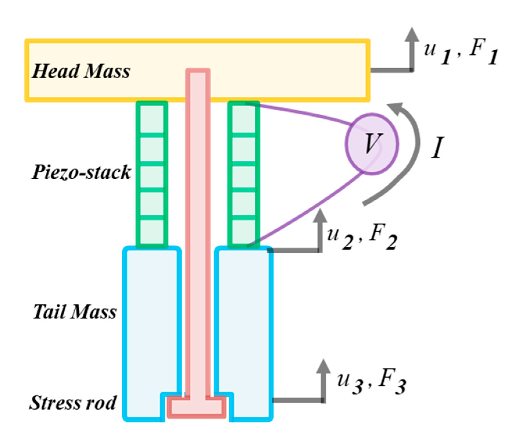
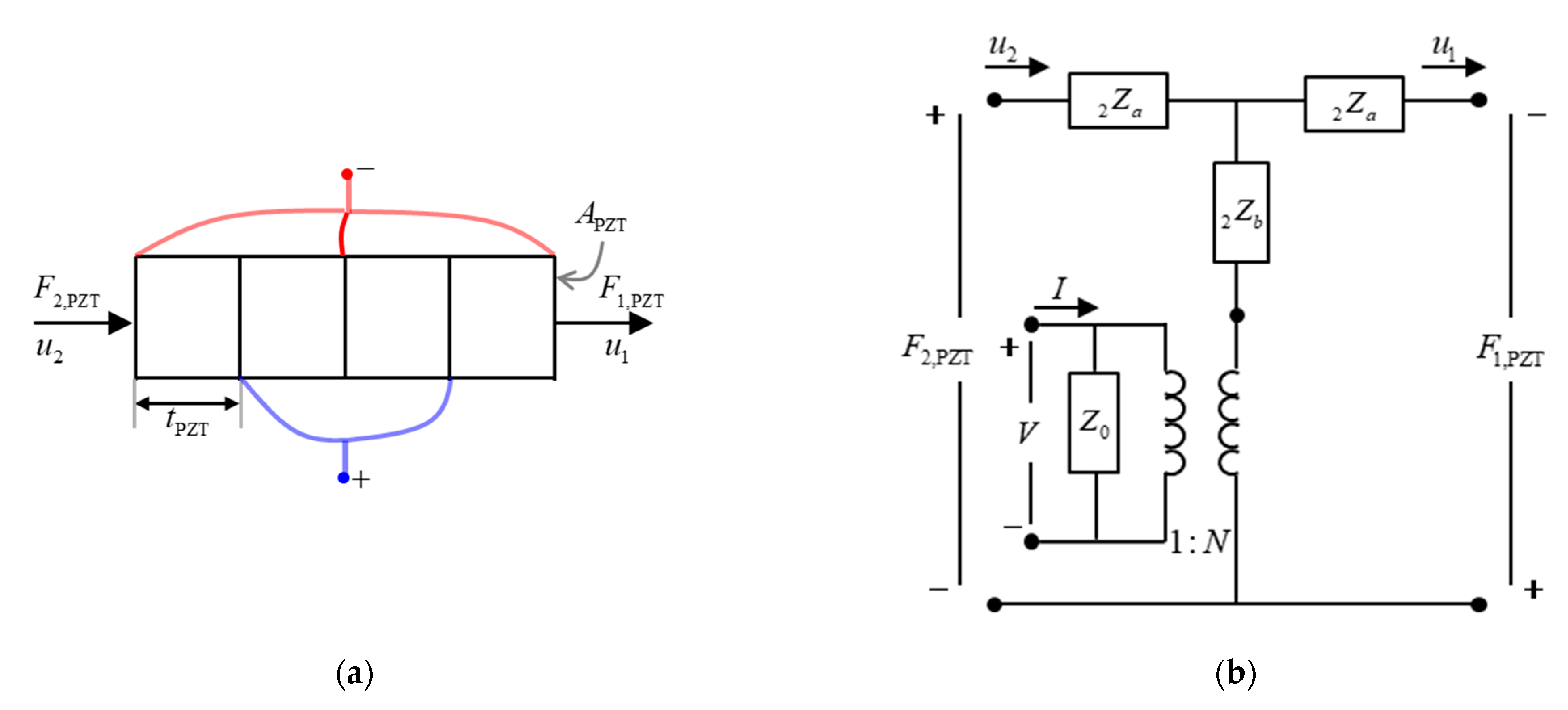
2.1. Impedance Matrix Equation

2.1.1. Single Transducer

Tonpilz transducers are piezoelectric transducers mainly used for relatively low frequencies and high-power sound emission. Figure 1 shows a free body diagram of a tonpilz transducer. The transducer consists of its four basic components: the piston head mass, piezoelectric stack, tail mass, and stress rod. $u_1$, $u_2$, and $u_3$ are the velocities, and $I$ is the current of a transducer. $F_1$, $F_2$, and $F_3$ are the forces, and $V$ is the driving voltage. Here, each force can be written as

$$\begin{array}{l}{F}_1=F_r+F_{1,\mathrm{Head}}+F_{1,\mathrm{PZT}}+F_{1,\mathrm{st}}\\ F_2=F_{2,\mathrm{PZT}}+F_{2,\mathrm{Tail}}\\ F_3=F_{3,\mathrm{Tail}}+F_{3,\mathrm{st}}\end{array}$$

(1)

where $F_r$ is the reaction force of the medium to the motion of the wet surface (the radiating surface) of the head mass, and $F_{1,\mathrm{Head}}$ is the inertia force of the head mass. $F_{1,\mathrm{PZT}}$ and $F_{2,\mathrm{PZT}}$ are the forces exerted by the piezoelectric stack on the top and bottom of the piezoelectric stack, respectively. $F_{1,\mathrm{st}}$ and $F_{3,\mathrm{st}}$ are the forces exerted by the stress rod on the top and bottom of the stress rod, respectively. $F_{2,\mathrm{Tail}}$ and $F_{3,\mathrm{Tail}}$ are the forces exerted by the tail mass on the top and bottom of the tail mass, respectively.

The transducer’s head mass is assumed to be rigid because it needs to provide uniform longitudinal motion, and its first flexural resonance should be significantly above the operating frequency band. Thus, the force $F_{1,\mathrm{Head}}$ and the mechanical impedance of the head mass $Z_1$ are expressed using the Lumped Parameter Model (LPM):

$$F_{1,\mathrm{Head}}=Z_1\hspace{0.17em}{u}_1\hspace{0.17em}\hspace{0.17em}\hspace{0.17em}\hspace{0.17em}\hspace{0.17em}\hspace{0.17em}\hspace{0.17em}\hspace{0.17em}\hspace{0.17em}\hspace{0.17em}where\hspace{0.17em}\hspace{0.17em}{Z}_1=\mathrm{j}\omega \hspace{0.17em}{M}_{\mathrm{Head}}$$

(2)

where $\mathrm{j}=\sqrt{-1}$, $\omega \hspace{0.17em}$ is the circular frequency, and $M_{\mathrm{Head}}$ is the mass of the head.

${}_{2}Z_c$, ${}_{2}Z_b$, ${}_{3}Z_c$, ${}_{3}Z_b$, ${}_{4}Z_c$ and ${}_{4}Z_b$ denote the mechanical impedances of the components of the transducer other than the head, obtained by the T-network. The right subscripts $b$ and $c$ indicate the shunt arm impedance and the sum of the shunt arm impedance and series arm impedance of the T-network, respectively. The left subscripts 2, 3, and 4 denote the components of the transducer: piezoelectric elements, tail, and stress rod, respectively.

The free body diagram and EC model of a piezoelectric stack are shown in Figure 2. From the EC model shown in Figure 2b, the following equations can be obtained.

$$\begin{array}{l}I\hspace{0.17em}\hspace{0.17em}\hspace{0.17em}\hspace{0.17em}\hspace{0.17em}\hspace{0.17em}\hspace{0.17em}=N(u_1-u_2)+\left(1/Z_0\right)V\\ F_{1,\mathrm{PZT}}=+{}_{2}Z_c{u}_1-{}_{2}Z_b{u}_2-NV\hspace{0.17em}\hspace{0.17em}\hspace{0.17em}\hspace{0.17em}\hspace{0.17em}\hspace{0.17em}\hspace{0.17em}\hspace{0.17em}\hspace{0.17em}\hspace{0.17em}\hspace{0.17em}\hspace{0.17em}\hspace{0.17em}\hspace{0.17em}\hspace{0.17em}\hspace{0.17em}\hspace{0.17em}\hspace{0.17em}\hspace{0.17em}where\hspace{0.17em}\hspace{0.17em}\hspace{0.17em}{}_{2}Z_c={}_{2}Z_a+{}_{2}Z_b\\ F_{2,\mathrm{PZT}}=-{}_{2}Z_b{u}_1+{}_{2}Z_c{u}_2+NV\end{array}$$

(3)

Using Equation (3), the following equations can be obtained.

$$\begin{array}{l}{F}_{1,\mathrm{PZT}}=\left(+{}_{2}Z_c+N^2{Z}_0\right)u_1+\left(-{}_{2}Z_b-N^2{Z}_0\right)u_2-N{Z}_{0}I\\ F_{2,\mathrm{PZT}}=\left(-{}_{2}Z_b-N^2{Z}_0\right)u_1+\left(+{}_{2}Z_c+N^2{Z}_0\right)u_2+N{Z}_{0}I\\ V\hspace{0.17em}\hspace{0.17em}\hspace{0.17em}\hspace{0.17em}\hspace{0.17em}\hspace{0.17em}\hspace{0.17em}=-N{Z}_0{u}_1+N{Z}_0{u}_2+Z_{0}I\end{array}$$

(4)

For a segmented 33 bar, the shunt electrical impedance $Z_0$ can be obtained from the geometry and material properties of the PZT (lead zirconate titanate) elements using the LPM:

$$\begin{array}{l}{Z}_0=1/\mathrm{j}\omega C_0\\ C_0=C_f(1-k_{33}^2)\\ C_f=n_{PZT}^{}{\epsilon }_{33}^T{A}_{PZT}/t_{PZT}\\ k_{33}^2=d_{33}^2/s_{33}^E{\epsilon }_{33}^T\\ N=d_{33}{A}_{PZT}/t{s}_{33}^E\end{array}$$

(5)

where $C_0^{}$ is the clamped capacitance, $C_f^{}$ is the free capacitance, $k_{33}^2$ is the coupling coefficient, $n_{\mathrm{PZT}}$ is the number of rings in the drive stacks, $t_{\mathrm{PZT}}$ is the thickness of each ring, $d_{33}$ is the piezoelectric coefficient, $A_{\mathrm{PZT}}$ is the cross-sectional area, $s_{33}^E$ is the elastic compliance coefficient, ${\epsilon }_{33}^T$ is the permittivity coefficient, and $N$ is the electromechanical turn ratio.

As shown in Figure 2b, the mechanical part of the EC model of a piezoelectric stack is represented using a T-network¹² based on a simple longitudinal bar model. The T-network is one of the ways to express a distributed parameter system as an EC model. The mechanical impedances of piezoelectric element ${}_{2}Z_c,\hspace{0.17em}\hspace{0.17em}{}_{2}Z_b$ can be written as

$$\begin{array}{l}{}_{2}Z_c=-\mathrm{j}{\rho }_{\mathrm{PZT}}{c}_{\mathrm{PZT}}{A}_{\mathrm{PZT}}\cot (k_{\mathrm{PZT}}{L}_{\mathrm{PZT}})\hspace{0.17em}\hspace{0.17em}\hspace{0.17em}\hspace{0.17em}\hspace{0.17em}\hspace{0.17em}\\ {}_{2}Z_b=-\mathrm{j}{\rho }_{\mathrm{PZT}}{c}_{\mathrm{PZT}}{A}_{\mathrm{PZT}}/sin(k_{\mathrm{PZT}}{L}_{\mathrm{PZT}})\hspace{0.17em}\hspace{0.17em}\hspace{0.17em}\hspace{0.17em}\hspace{0.17em}\hspace{0.17em}\hspace{0.17em}\hspace{0.17em}\hspace{0.17em}\hspace{0.17em}\hspace{0.17em}\hspace{0.17em}\hspace{0.17em}\hspace{0.17em}\hspace{0.17em}\hspace{0.17em}\hspace{0.17em}\hspace{0.17em}\hspace{0.17em}\end{array}$$

(6)

where $\rho ,\hspace{0.17em}\hspace{0.17em}c,\hspace{0.17em}\hspace{0.17em}A$, and $L$ are the density, wave velocity, cross-sectional area, and longitudinal length of the part, respectively. $k$ is the wave number. The subscripts PZT denote the piezoelectric stack.

The tail mass and stress rod have the same form of T-network EC model as the PZT stack, except that there is no electrical part. Thus, the following equations can be obtained in a similar way:

$$\begin{array}{l}{F}_{2,\mathrm{Tail}}=+{}_{3}Z_c{u}_2-{}_{3}Z_b{u}_3\\ F_{3,\mathrm{Tail}}=-{}_{3}Z_b{u}_2+{}_{3}Z_c{u}_3\\ F_{1,\mathrm{st}}\hspace{0.17em}\hspace{0.17em}\hspace{0.17em}=+{}_{4}Z_c{u}_1-{}_{4}Z_b{u}_3\\ F_{3,\mathrm{st}}\hspace{0.17em}\hspace{0.17em}\hspace{0.17em}=-{}_{4}Z_b{u}_1+{}_{4}Z_c{u}_3\end{array}$$

(7)

The mechanical impedances of tail mass ${}_{3}Z_c,\hspace{0.17em}\hspace{0.17em}{}_{3}Z_b$ and the mechanical impedances of stress rod ${}_{4}Z_c,\hspace{0.17em}\hspace{0.17em}{}_{4}Z_b$ can be written as

$$\begin{array}{l}{}_{3}Z_c=-\mathrm{j}{\rho }_{\mathrm{Tail}}{c}_{\mathrm{Tail}}{A}_{\mathrm{Tail}}\cot (k_{\mathrm{Tail}}{L}_{\mathrm{Tail}})\hspace{0.17em}\hspace{0.17em}\hspace{0.17em}\hspace{0.17em}\hspace{0.17em}\hspace{0.17em}\hspace{0.17em}\hspace{0.17em}\hspace{0.17em}\hspace{0.17em}\hspace{0.17em}\hspace{0.17em}\\ {}_{3}Z_b=-\mathrm{j}{\rho }_{\mathrm{Tail}}{c}_{\mathrm{Tail}}{A}_{\mathrm{Tail}}/\sin (k_{\mathrm{Tail}}{L}_{\mathrm{Tail}})\hspace{0.17em}\hspace{0.17em}\hspace{0.17em}\hspace{0.17em}\hspace{0.17em}\hspace{0.17em}\hspace{0.17em}\hspace{0.17em}\hspace{0.17em}\hspace{0.17em}\hspace{0.17em}\hspace{0.17em}\hspace{0.17em}\hspace{0.17em}\hspace{0.17em}\\ {}_{4}Z_c=-\mathrm{j}{\rho }_{\mathrm{st}}{c}_{\mathrm{st}}{A}_{\mathrm{st}}\cot (k_{\mathrm{st}}{L}_{\mathrm{st}})\hspace{0.17em}\hspace{0.17em}\hspace{0.17em}\hspace{0.17em}\hspace{0.17em}\hspace{0.17em}\hspace{0.17em}\hspace{0.17em}\hspace{0.17em}\hspace{0.17em}\hspace{0.17em}\hspace{0.17em}\hspace{0.17em}\hspace{0.17em}\hspace{0.17em}\hspace{0.17em}\hspace{0.17em}\hspace{0.17em}\hspace{0.17em}\hspace{0.17em}\hspace{0.17em}\hspace{0.17em}\hspace{0.17em}\hspace{0.17em}\hspace{0.17em}\\ {}_{4}Z_b=-\mathrm{j}{\rho }_{\mathrm{st}}{c}_{\mathrm{st}}{A}_{\mathrm{st}}/\sin (k_{\mathrm{st}}{L}_{\mathrm{st}})\hspace{0.17em}\hspace{0.17em}\hspace{0.17em}\hspace{0.17em}\hspace{0.17em}\hspace{0.17em}\hspace{0.17em}\hspace{0.17em}\hspace{0.17em}\hspace{0.17em}\hspace{0.17em}\hspace{0.17em}\hspace{0.17em}\hspace{0.17em}\hspace{0.17em}\hspace{0.17em}\hspace{0.17em}\hspace{0.17em}\hspace{0.17em}\hspace{0.17em}\hspace{0.17em}\hspace{0.17em}\hspace{0.17em}\hspace{0.17em}\hspace{0.17em}\hspace{0.17em}\hspace{0.17em}\end{array}$$

(8)

Here, the subscripts Tail, and st denote the parts of the transducer.

The reaction force of the medium to the motion of the head surface $F_r$ is

$$F_r=\underset{S}{\mathsf{\iint }}p(\overrightarrow{r})dS$$

(9)

where $S$ is the wet surface (the radiating surface) of the transducer head, $\overrightarrow{r}$ is the position vector on the radiating surface, and $p(\overrightarrow{r})$ is the pressure produced by the transducer head. For a single transducer, $F_r$ can be expressed in terms of the self-radiation impedance $Z_r$ by dividing by the velocity of the head $u_1$:

$$Z_r=\frac{F_r}{u_1}\hspace{0.17em}\hspace{0.17em}\hspace{0.17em}\hspace{0.17em}\hspace{0.17em}\hspace{0.17em}\hspace{0.17em}\hspace{0.17em}\hspace{0.17em}\hspace{0.17em}\hspace{0.17em}\hspace{0.17em}\hspace{0.17em}where\hspace{0.17em}\hspace{0.17em}\hspace{0.17em}\hspace{0.17em}{Z}_r=\frac{1}{u_1}\underset{S}{\iint }p(\overrightarrow{r})dS$$

(10)

By using the Equations (1), (2), (4), (7) and (10), the impedance matrix equation for a single tonpilz transducer can be expressed as

$$Zu=F$$

(11)

where $Z$ is the impedance matrix, $u$ is a vector of velocities and current of the transducer, and $F$ is a vector of the external forces and voltage of the transducer. They can be written as

$$Z=\left[\begin{array}{cccc}{Z}_r+Z_1+{}_{2}Z_c+{}_{4}Z_c+N^2{Z}_0& -{}_{2}Z_b-N^2{Z}_0& -{}_{4}Z_b& -N{Z}_0\\ -{}_{2}Z_b-N^2{Z}_0& {}_{2}Z_c+{}_{3}Z_c+N^2{Z}_0& -{}_{3}Z_b& +N{Z}_0\\ -{}_{4}Z_b& -{}_{3}Z_b& {}_3{Z}_c+{}_{4}Z_c& 0\\ \hspace{0.17em}\hspace{0.17em}-N\hspace{0.17em}{Z}_0& +N{Z}_0& 0& Z_0\end{array}\right]$$

(12)

$$u={\left[\begin{array}{cccc}{u}_1& u_2& u_3& I\end{array}\right]}^{\mathrm{T}},\hspace{0.17em}\hspace{0.17em}\hspace{0.17em}\hspace{0.17em}\hspace{0.17em}\hspace{0.17em}\hspace{0.17em}\hspace{0.17em}\hspace{0.17em}\hspace{0.17em}\hspace{0.17em}\hspace{0.17em}\hspace{0.17em}F={\left[\begin{array}{cccc}{F}_1& F_2& F_3& V\end{array}\right]}^{\mathrm{T}}$$

(13)

2.1.2. Array of Transducers

For an array of transducers, depending on where the transducer is in the array, the reaction force of the medium, $F_r$, has different characteristics. The force exerted on the ith transducer, $F_{r,i}$, by the pressures from all the transducers is

$$F_{r,i}=\sum _{k=1}^n\underset{S}{\iint }{p}_k({\overrightarrow{r}}_{ik})d{S}_i$$

(14)

where $n$ is the number of transducers that make up the array, $S_i$ is the wet surface of the ith transducer head, $p_k({\overrightarrow{r}}_{ik})$ is the pressure produced by the kth transducer at the designated point on ith transducer, and $r_{ik}$ is the distance from the center of the kth transducer to the designated point. This force, $F_{r,i}$, can be expressed in terms of the radiation impedance, $Z_{r,i}$, of the ith transducer by dividing by the velocity of that transducer head, $u_{1,i}$, as was done for a single transducer in Equation (10):

$$Z_{r,i}=\frac{F_{r,i}}{u_{1,i}}=\frac{1}{u_{1,i}}\sum _{k=1}^n\underset{S}{\iint }{p}_k({\overrightarrow{r}}_{ik})d{S}_i=\frac{1}{u_{1,i}}\sum _{k=1}^n{u}_{1,k}{Z}_{r,ik}\hspace{0.17em}\hspace{0.17em}\hspace{0.17em}\hspace{0.17em}\hspace{0.17em}\hspace{0.17em}\hspace{0.17em}\hspace{0.17em}\hspace{0.17em}\hspace{0.17em}\hspace{0.17em}\hspace{0.17em}\hspace{0.17em}\hspace{0.17em}where\hspace{0.17em}\hspace{0.17em}\hspace{0.17em}\hspace{0.17em}{Z}_{r,ik}=\frac{1}{u_{1,k}}\underset{S}{\iint }{p}_k({\overrightarrow{r}}_{ik})d{S}_i$$

(15)

Here, $Z_{r,ik}$ is defined as the mutual radiation impedance between the ith and kth transducer, and $u_{1,k}$ is the velocity of kth transducer head. Equation (15) shows that the coupling between transducers occurs in the acoustic region and can be expressed as mutual radiation impedance.

Generally, the transducers that make up an array are all the same transducers, so when constructing the impedance matrix of an array, all transducers have the same electrical and mechanical impedance. Thus, the impedance matrix equation of the ith transducer can be expressed as

$$Z_i{u}_i=F_i$$

(16)

where $Z_i$ is the impedance matrix of the ith transducer, $u_i$ is a vector of velocities and current of the ith transducer, and $F_i$ is a vector of the forces and voltage of the ith transducer. They can be written as

$$Z_i=\left[\begin{array}{cccc}{Z}_{r,i}+Z_1+{}_{2}Z_c+{}_{4}Z_c+N^2{Z}_0& -{}_{2}Z_b-N^2{Z}_0& -{}_{4}Z_b& -N{Z}_0\\ -{}_{2}Z_b-N^2{Z}_0& {}_{2}Z_c+{}_{3}Z_c+N^2{Z}_0& -{}_{3}Z_b& +N{Z}_0\\ -{}_{4}Z_b& -{}_{3}Z_b& {}_3{Z}_c+{}_{4}Z_c& 0\\ \hspace{0.17em}\hspace{0.17em}-N\hspace{0.17em}{Z}_0& +N{Z}_0& 0& Z_0\end{array}\right]$$

(17)

$$u_i={\left[{\begin{array}{cccc}{u}_{1,i}& u_{2,i}& u_{3,i}& I\end{array}}_i\right]}^{\mathrm{T}},\hspace{0.17em}\hspace{0.17em}\hspace{0.17em}\hspace{0.17em}\hspace{0.17em}\hspace{0.17em}\hspace{0.17em}\hspace{0.17em}\hspace{0.17em}\hspace{0.17em}\hspace{0.17em}\hspace{0.17em}\hspace{0.17em}{F}_i={\left[\begin{array}{cccc}{F}_{1,i}& F_{2,i}& F_{3,i}& V_i\end{array}\right]}^{\mathrm{T}}$$

(18)

where $u_{1,i}$, $u_{2,i}$ and $u_{3,i}$ are the velocities, and $I_i$ is the current of the ith transducer. $F_{1,i}$, $F_{2,i}$ and $F_{3,i}$ are the forces, and $V_i$ is the driving voltage of the ith transducer. Substituting Equation (15) into $Z_{r,i}$ of Equation (17), the impedance matrix equation for the array of transducers can be derived as

$$\begin{array}{l}\left[\begin{array}{ccc}{\tilde{Z}}_{11}& \cdots & {\tilde{Z}}_{1n}\\ ⋮& \ddots & ⋮\\ {\tilde{Z}}_{n1}& \cdots & {\tilde{Z}}_{nn}\end{array}\right]\left\{\begin{array}{c}{u}_1\\ ⋮\\ u_n\end{array}\right\}=\left\{\begin{array}{c}{F}_1\\ ⋮\\ F_n\end{array}\right\}\hspace{0.17em}\hspace{0.17em}\hspace{0.17em}\hspace{0.17em}\hspace{0.17em}\hspace{0.17em}\hspace{0.17em}\hspace{0.17em}\hspace{0.17em}\hspace{0.17em}\hspace{0.17em}\hspace{0.17em}\hspace{0.17em}\hspace{0.17em}\hspace{0.17em}or\hspace{0.17em}\hspace{0.17em}\hspace{0.17em}\hspace{0.17em}\hspace{0.17em}\hspace{0.17em}\hspace{0.17em}\hspace{0.17em}\hspace{0.17em}\hspace{0.17em}\hspace{0.17em}\hspace{0.17em}\hspace{0.17em}\hspace{0.17em}\hspace{0.17em}{\displaystyle \sum _{k=1}^n{\tilde{Z}}_{ik}{u}_k}=F_i\\ where\hspace{0.17em}\hspace{0.17em}\hspace{0.17em}{\tilde{Z}}_{ik}=\left[\begin{array}{cccc}{Z}_{r,ik}& 0& 0& 0\\ 0& 0& 0& 0\\ 0& 0& 0& 0\\ 0& 0& 0& 0\end{array}\right]+\left[\begin{array}{cccc}{Z}_1+{}_{2}Z_c+{}_{4}Z_c+N^2{Z}_0& -{}_{2}Z_b-N^2{Z}_0& -{}_{4}Z_b& -N{Z}_0\\ -{}_{2}Z_b-N^2{Z}_0& {}_{2}Z_c+{}_{3}Z_c+N^2{Z}_0& -{}_{3}Z_b& +N{Z}_0\\ -{}_{4}Z_b& -{}_{3}Z_b& {}_3{Z}_c+{}_{4}Z_c& 0\\ \hspace{0.17em}\hspace{0.17em}-N\hspace{0.17em}{Z}_0& +N{Z}_0& 0& Z_0\end{array}\right]{\delta }_{ik}\end{array}$$

(19)

where ${\delta }_{ik}$ is the Kronecker delta, and ${\tilde{Z}}_{ik}$ is an impedance matrix representing the relation between the ith transducer and the kth transducer.

2.2. Acoustic Radiation Impedance

In this study, an FE-BE coupling method has been developed to calculate the acoustic mutual-radiation impedance, $Z_{r,ik}$, for an array of transducers with surrounding structures. This is done to reflect the influence of the vibration mode of the elastic surrounding structures and the influence of sound wave transmission and refraction by the surrounding structures on the impedance.

In this section, the formulations used are based on the coupling of the FE for the structure and the BE for the fluid. The FE/BE coupling method leads to reduction of the computational resources compared to when using the conventional FE model.

When an elastic structure of arbitrary shape is immersed in the fluid as shown in Figure 3a, the finite element modeling of the structure is given by the following discretized governing equation [34]:

$$Z_s{v}_s=F_s-GQSp\hspace{0.17em}\hspace{0.17em}\hspace{0.17em}\hspace{0.17em}\hspace{0.17em}\hspace{0.17em}\hspace{0.17em}\hspace{0.17em}\hspace{0.17em}\hspace{0.17em}\hspace{0.17em}\hspace{0.17em}\hspace{0.17em}\hspace{0.17em}where\hspace{0.17em}\hspace{0.17em}\hspace{0.17em}\hspace{0.17em}{Z}_s=\mathrm{j}\omega M+C+\frac{K}{\mathrm{j}\omega }$$

(20)

where $M$, $C$ and $K$ are the mass, damping, and stiffness matrices of the elastic structure obtained by the FEM, respectively. $v_s$ is a velocity vector corresponding to all DOFs of the structure. $F_s$ is the harmonic load vector for the structure. $G$ is a matrix that is used to find nodes on the surface (wet surface) where the elastic structure is in contact with the acoustic medium. $Q$ is a transformation matrix that converts the outward unit normal force of the nodes on the wet surface to the force of the node in the fixed coordinate system (the global coordinate system). $S$ is a diagonal matrix where the diagonal elements are the areas of each element on the wet surface of the elastic structure. $p$ is the surface pressure acting on the radiating surface.

In this study, Equation (20) has been developed in the form necessary to obtain the acoustic radiation impedance of an array. When an elastic surrounding structure of arbitrary shape is placed around the radiating surface of the array as shown in Figure 3b, the finite element modeling of the surrounding structure is given by the following discretized governing equation:

$$Z_s{v}_s=F_s-G_2{Q}_2{S}_2{p}_2-G_3{Q}_3{S}_3{p}_3\hspace{0.17em}\hspace{0.17em}\hspace{0.17em}\hspace{0.17em}$$

(21)

where $p_2$$\left(s_2\times 1\right)$ is the surface pressure acting on the radiating surface when the elastic structure and fluid 1 come into contact, as shown in Figure 3b. $p_3$$\left(s_3\times 1\right)$ is the surface pressure acting on the radiating surface when the elastic structure and fluid 2 come into contact. $S_2$$\left(s_2\times s_2\right)$ and $S_3$$\left(s_3\times s_3\right)$ are the area matrices of the inner and outer surfaces of the elastic surrounding structure, respectively. $G_2$$\left(s_0\times 3s_2\right)$ and $G_3$$\left(s_0\times 3s_3\right)$ are transformation matrixes of the inner and outer surfaces of the elastic surrounding structure, respectively. $Q_2$$\left(3s_2\times s_2\right)$ and $Q_3$$\left(3s_3\times s_3\right)$ are transformation matrixes of the inner and outer surfaces of the elastic surrounding structure, respectively. Using this transformation matrix, the velocities $v_{n2}$$\left(s_2\times 1\right)$ and $v_{n3}$$\left(s_2\times 1\right)$ in the normal direction of the radiating surface can be expressed as the following equation in the fixed coordinate system:

$$v_{n2}=Q_2^T{v}_2\hspace{0.17em}\hspace{0.17em}\hspace{0.17em}\hspace{0.17em}\hspace{0.17em}\hspace{0.17em}\hspace{0.17em},\hspace{0.17em}\hspace{0.17em}\hspace{0.17em}\hspace{0.17em}\hspace{0.17em}\hspace{0.17em}\hspace{0.17em}\hspace{0.17em}\hspace{0.17em}\hspace{0.17em}\hspace{0.17em}\hspace{0.17em}\hspace{0.17em}\hspace{0.17em}\hspace{0.17em}{v}_{n3}=Q_3^T{v}_3$$

(22)

where $v_2$ and $v_3$ are the velocity vectors corresponding to the DOFs of the structure on the inner and outer wet surfaces of the structure, respectively. As these velocity vectors are included in $v_s$, the velocity vector $v_s$ and the corresponding harmonic load vector $F_s$ can be expressed as follows:

$$v_s={\left[v_2,\hspace{0.17em}{v}_{in},\hspace{0.17em}{v}_3\right]}^{\mathrm{T}},\hspace{0.17em}\hspace{0.17em}\hspace{0.17em}\hspace{0.17em}\hspace{0.17em}\hspace{0.17em}\hspace{0.17em}\hspace{0.17em}\hspace{0.17em}\hspace{0.17em}{F}_s={\left[F_2,\hspace{0.17em}{F}_{in},\hspace{0.17em}{F}_3\right]}^{\mathrm{T}}$$

(23)

The subscript $in$ denotes that the value is not on the wet surface. $s_0,\hspace{0.17em}\hspace{0.17em}{s}_1,\hspace{0.17em}\hspace{0.17em}{s}_2$ and $s_3$, indicating the sizes of each matrix, are the DOFs of the structure, the DOF of the fluid on the outer surface of the array, the DOFs of fluid 1 on the inner surface of the surrounding structure, and the DOFs of fluid 2 on the outer surface of the surrounding structure, respectively.

Next, fluid 1 between the array and the surrounding structure and fluid 2 outside the surrounding structure satisfy the Helmholtz equation. The radiating surface is divided into boundary elements, and the fluid is modeled and formulated. Using the acoustic BEM, the relation between the surface pressure and the normal surface velocity of the radiating surface is given by the following equation:

$$\begin{array}{c}\left[\begin{array}{cc}{B}_{1,11}& B_{1,12}\\ B_{1,21}& B_{1,22}\end{array}\right]\left\{\begin{array}{c}{v}_{n1}\\ v_{n2}\end{array}\right\}-\left[\begin{array}{cc}{A}_{1,11}& A_{1,12}\\ A_{1,21}& A_{1,22}\end{array}\right]\left\{\begin{array}{c}{p}_1\\ p_2\end{array}\right\}=\left\{\begin{array}{c}0\\ 0\end{array}\right\}\hspace{0.17em}\hspace{0.17em}\hspace{0.17em}\hspace{0.17em}\hspace{0.17em}\hspace{0.17em}\hspace{0.17em}\hspace{0.17em}\hspace{0.17em}\hspace{0.17em}\hspace{0.17em}\hspace{0.17em}\hspace{0.17em}\hspace{0.17em}\hspace{0.17em}\hspace{0.17em}\hspace{0.17em}\hspace{0.17em}\hspace{0.17em}\hspace{0.17em}\hspace{0.17em}\hspace{0.17em}\hspace{0.17em}\hspace{0.17em}\hspace{0.17em}\\ \hspace{0.17em}\hspace{0.17em}\hspace{0.17em}\hspace{0.17em}where\hspace{0.17em}\hspace{0.17em}\hspace{0.17em}\left[B_1\right]=\left[\begin{array}{cc}{B}_{1,11}& B_{1,12}\\ B_{1,21}& B_{1,22}\end{array}\right],\hspace{0.17em}\hspace{0.17em}\hspace{0.17em}\hspace{0.17em}\hspace{0.17em}\hspace{0.17em}\left[A_1\right]=\left[\begin{array}{cc}{A}_{1,11}& A_{1,12}\\ A_{1,21}& A_{1,22}\end{array}\right]\end{array}\hspace{0.17em}\hspace{0.17em}\hspace{0.17em}\hspace{0.17em}\hspace{0.17em}\hspace{0.17em}\hspace{0.17em}\hspace{0.17em}in\hspace{0.17em}fluid\hspace{0.17em}1$$

(24)

$$B_2\hspace{0.17em}{v}_{n3}-A_2\hspace{0.17em}{p}_3=\left\{0\right\}\hspace{0.17em}\hspace{0.17em}\hspace{0.17em}\hspace{0.17em}\hspace{0.17em}\hspace{0.17em}\hspace{0.17em}\hspace{0.17em}\hspace{0.17em}\hspace{0.17em}\hspace{0.17em}\hspace{0.17em}\hspace{0.17em}\hspace{0.17em}\hspace{0.17em}\hspace{0.17em}\hspace{0.17em}\hspace{0.17em}\hspace{0.17em}\hspace{0.17em}\hspace{0.17em}\hspace{0.17em}\hspace{0.17em}\hspace{0.17em}\hspace{0.17em}\hspace{0.17em}\hspace{0.17em}\hspace{0.17em}\hspace{0.17em}\hspace{0.17em}\hspace{0.17em}\hspace{0.17em}\hspace{0.17em}\hspace{0.17em}\hspace{0.17em}\hspace{0.17em}\hspace{0.17em}\hspace{0.17em}\hspace{0.17em}\hspace{0.17em}\hspace{0.17em}\hspace{0.17em}\hspace{0.17em}\hspace{0.17em}\hspace{0.17em}\hspace{0.17em}\hspace{0.17em}\hspace{0.17em}\hspace{0.17em}\hspace{0.17em}\hspace{0.17em}\hspace{0.17em}\hspace{0.17em}\hspace{0.17em}\hspace{0.17em}\hspace{0.17em}\hspace{0.17em}\hspace{0.17em}\hspace{0.17em}\hspace{0.17em}\hspace{0.17em}\hspace{0.17em}\hspace{0.17em}\hspace{0.17em}\hspace{0.17em}\hspace{0.17em}\hspace{0.17em}\hspace{0.17em}\hspace{0.17em}\hspace{0.17em}in\hspace{0.17em}fluid\hspace{0.17em}2$$

(25)

where $v_{n1}$$\left(s_1\times 1\right)$ and $p_1$$\left(s_1\times 1\right)$ are the normal velocity and the surface pressure acting on the radiating surface on the array, respectively. $\left[A_1\right]$ and $\left[B_1\right]$ are the dipole and monopole matrices obtained by the BEM for the fluid 1 between the array and the surrounding structure, respectively. $\left[A_2\right]$ and $\left[B_2\right]$ are the dipole and monopole matrices obtained by the BEM for the fluid 2 outside the surrounding structure, respectively. These matrices are dependent on the frequency, geometry, and fluid properties.

Finally, the governing matrix equation of the structure–fluid coupling system can be obtained by combining Equations (21), (24) and (25):

$$\left[\begin{array}{ccccccc}0& & & & 0& & \\ 0& & Z_s& & 0& G_2{Q}_2{S}_2& G_3{Q}_3{S}_3\\ 0& & & & 0& & \\ B_{1,11}& B_{1,12}{Q}_2^T& 0& 0& -A_{1,11}& -A_{1,12}& 0\\ B_{1,21}& B_{1,22}{Q}_2^T& 0& 0& -A_{1,21}& -A_{1,22}& 0\\ 0& 0& 0& B_2{Q}_3^T& 0& 0& -A_2\end{array}\right]\left\{\begin{array}{c}{v}_{n1}\\ v_2\\ v_{in}\\ v_3\\ p_1\\ p_2\\ p_3\end{array}\right\}=\left\{\begin{array}{c}{F}_2\\ F_{in}\\ F_3\\ 0\\ 0\\ 0\end{array}\right\}$$

(26)

Assuming that there is no external force to excite the structure ($F_s\hspace{0.17em}=\left\{0\right\}$), moving known values ($v_{n1}$) to the right side it can be expressed as the following equation.

$$\left[\begin{array}{cccccc}& & & 0& & \\ & Z_s& & 0& G_2{Q}_2^{}{S}_2& G_3{Q}_3^{}{S}_3\\ & & & 0& & \\ B_{1,12}{Q}_2^T& 0& 0& -A_{1,11}& -A_{1,12}& 0\\ B_{1,22}{Q}_2^T& 0& 0& -A_{1,21}& -A_{1,12}& 0\\ 0& 0& B_2{Q}_3^T& 0& 0& -A_2\end{array}\right]\left\{\begin{array}{c}{v}_2\\ v_{in}\\ v_3\\ p_1\\ p_2\\ p_3\end{array}\right\}=-\left[\begin{array}{c}0\\ 0\\ 0\\ B_{1,11}\\ B_{1,21}\\ 0\end{array}\right]\left\{v_{n1}\right\}$$

(27)

Now, $Z_{r,ik}$ can be obtained by the following process. First, by putting $v_{n1}$ in Equation (28) and substituting it into the equation above, we can obtain the dynamic behavior of the elastic surrounding structure $v_s$, the pressures of the radiating surface of the surrounding structures $p_2$ and $p_2$, and the pressure on the array surface $p_1$.

$$v_{n1,j}=\left\{\begin{array}{l}1,\hspace{0.17em}\hspace{0.17em}\hspace{0.17em}\hspace{0.17em}\hspace{0.17em}\hspace{0.17em}j\hspace{0.17em}\hspace{0.17em}\mathrm{is}\hspace{0.17em}\mathrm{on}\hspace{0.17em}\mathrm{the}\hspace{0.17em}\mathrm{surface}\hspace{0.17em}\mathrm{of} \mathrm{the}\hspace{0.17em}k\mathrm{th}\hspace{0.17em}\mathrm{transducer}\hspace{0.17em}\mathrm{head}\\ 0,\hspace{0.17em}\hspace{0.17em}\hspace{0.17em}\hspace{0.17em}\hspace{0.17em}\hspace{0.17em}j\hspace{0.17em}\mathrm{isn}’\mathrm{t}\hspace{0.17em}\mathrm{on}\hspace{0.17em}\mathrm{the}\hspace{0.17em}\mathrm{surface}\hspace{0.17em}\mathrm{of} \mathrm{the}\hspace{0.17em}k\mathrm{th}\hspace{0.17em}\mathrm{transducer}\hspace{0.17em}\mathrm{head}\end{array}\right.$$

(28)

where $v_{n1,j}$ is the jth element of $\left\{v_{n1}\right\}$. Then, $Z_{r,ik}$ can be obtained by postprocessing the obtained surface pressure $p_1$ according to the definition of the acoustic mutual radiation impedance as follows:

$$\begin{array}{ll}{Z}_{r,ik}=& \sum _{j=1}^{s_1}{S}_j{p}_{1j}{\mathsf{\Delta }}_j\\ & where\hspace{0.17em}\hspace{0.17em}\hspace{0.17em}{\mathsf{\Delta }}_j=\left\{\begin{array}{l}1,\hspace{0.17em}\hspace{0.17em}\hspace{0.17em}\hspace{0.17em}\hspace{0.17em}j\hspace{0.17em}\hspace{0.17em}\mathrm{is}\hspace{0.17em}\mathrm{on}\hspace{0.17em}\mathrm{the}\hspace{0.17em}\mathrm{surface}\hspace{0.17em}\mathrm{of}\hspace{0.17em}\mathrm{the}\hspace{0.17em}\mathrm{the}\hspace{0.17em}\hspace{0.17em}i\mathrm{th}\hspace{0.17em}\mathrm{transducer}\hspace{0.17em}\mathrm{head}\\ 0,\hspace{0.17em}\hspace{0.17em}\hspace{0.17em}j\hspace{0.17em}\hspace{0.17em}\mathrm{isn}’\mathrm{t}\hspace{0.17em}\mathrm{on}\hspace{0.17em}\mathrm{the}\hspace{0.17em}\mathrm{surface}\hspace{0.17em}\mathrm{of}\hspace{0.17em}\mathrm{the}\hspace{0.17em}\mathrm{the}\hspace{0.17em}\hspace{0.17em}i\mathrm{th}\hspace{0.17em}\mathrm{transducer}\hspace{0.17em}\mathrm{head}\end{array}\right.\end{array}$$

(29)

where $S_j$ is the area of the jth boundary element.

2.3. Transfer Matrix for Field Point Pressure Calculation

The acoustic pressure field radiated from an array can be obtained by the acoustic transfer matrix and the velocity distribution over the transducer heads calculated by the impedance matrix equation in Equation (19). The transfer matrix, $H$, indicates the transfer function between the surface velocity of transducer heads, $u_h$, and the pressure of field points, $P_f$:

$$P_f=H{u}_h\hspace{0.17em}\hspace{0.17em}\hspace{0.17em}\hspace{0.17em}\hspace{0.17em}\hspace{0.17em}\hspace{0.17em}\hspace{0.17em}\hspace{0.17em}\hspace{0.17em}\hspace{0.17em}\hspace{0.17em}\hspace{0.17em}\hspace{0.17em}\hspace{0.17em}\hspace{0.17em}\hspace{0.17em}where\hspace{0.17em}\hspace{0.17em}\hspace{0.17em}\hspace{0.17em}{u}_h={\left[\begin{array}{cccc}{u}_{1,1}& u_{1,2}& \cdots & u_{1,n}\end{array}\right]}^{\mathrm{T}}$$

(30)

The vector $P_f$$\left(m\times 1\right)$ is the pressure of the field points located in the area of interest. The vector $u_h$$\left(n\times 1\right)$ is the velocity of the transducer heads. The relation between the velocity of the transducer heads, $u_h$, and the surface normal velocity, $v_{n1}$, is shown in Equation (31):

$$v_{n1}=L_h{u}_h$$

(31)

where $L_h$$\left(s_1\times n\right)$ is a matrix for finding nodes on the surfaces of the transducer head on the radiating surface of the array.

The pressure of the field points, $P_f$, can be determined using the surface normal velocity $v_{n3}$ and the surface pressure $p_3$:

$$P_f=C_2\hspace{0.17em}{p}_3+D_2\hspace{0.17em}{v}_{n3}$$

(32)

where $\left[C_2\right]$ and $\left[D_2\right]$ are the dipole matrix and monopole matrix, respectively, for fluid 2 corresponding to the field points, obtained by the acoustic BEM. Equation (33) shows the relationship between the surface normal velocity, $v_{n1}$, and the structure velocity of outer surface, $v_3$. The transformation matrix $T$ between $v_{n1}$ and $v_3$ can be obtain from Equation (27).

$$v_3=T{v}_{n1}$$

(33)

By using Equations (22), (25), (31) and (33), Equation (32) can be expressed as

$$P_f=\left(C_2{A}_2^{-1}{B}_2+D_2\right)Q_3^T\hspace{0.17em}T\hspace{0.17em}{L}_h\hspace{0.17em}{u}_h$$

(34)

Thus, when there are surrounding structures, the transfer matrix $H$ is

$$H=\left(C_2{A}_2^{-1}{B}_2+D_2\right)Q_3^T\hspace{0.17em}T\hspace{0.17em}{L}_h$$

(35)

3. Validation

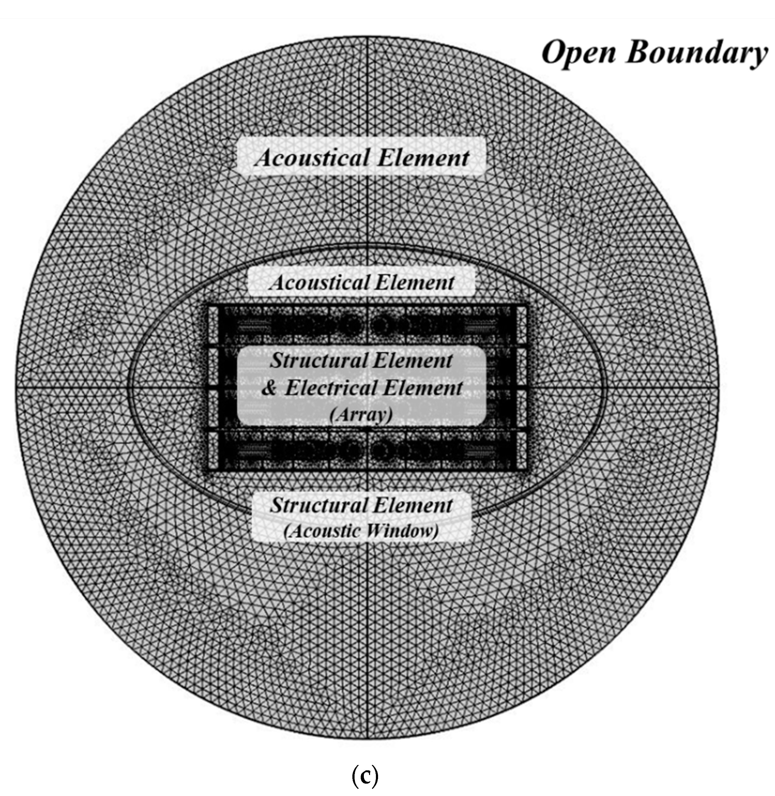
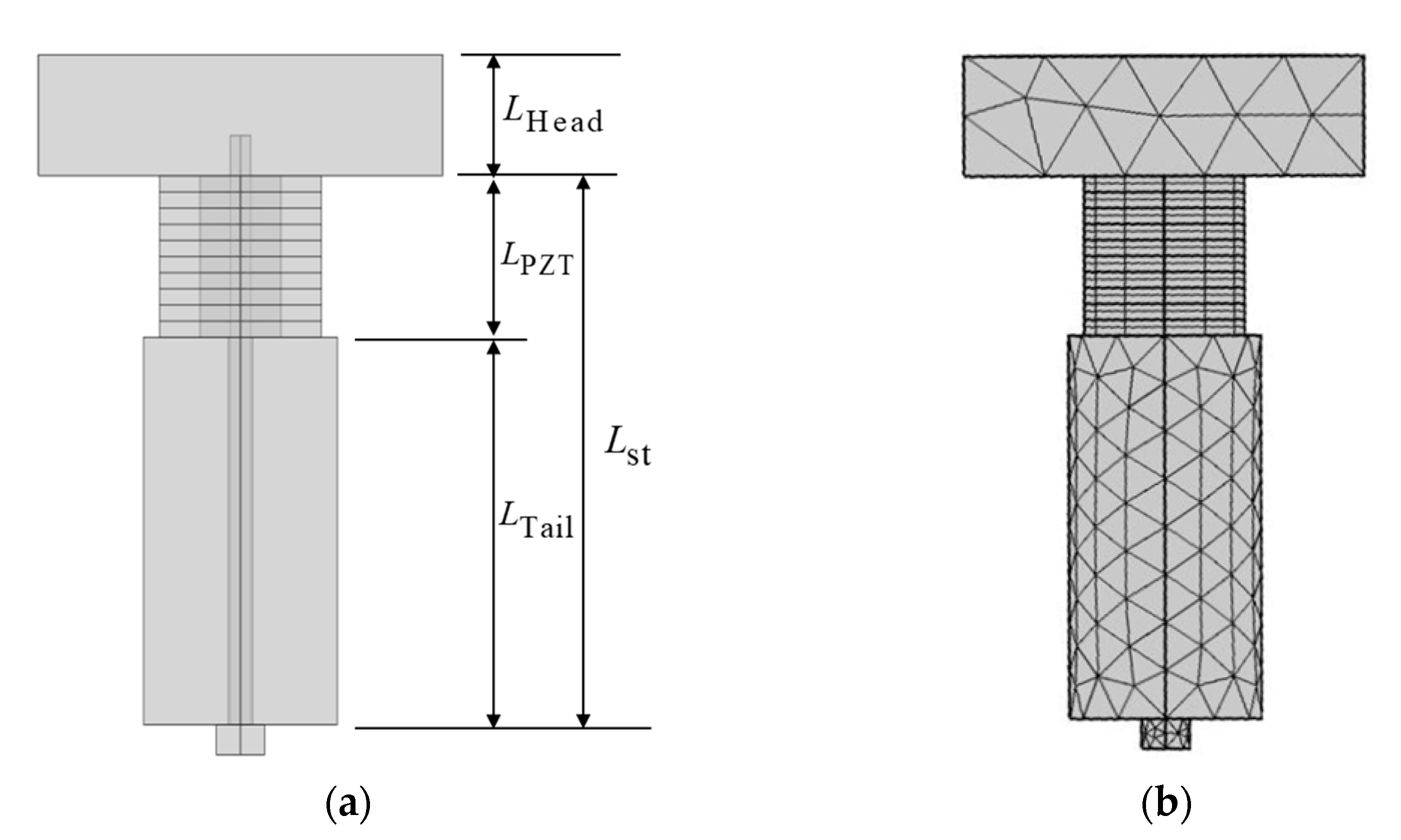
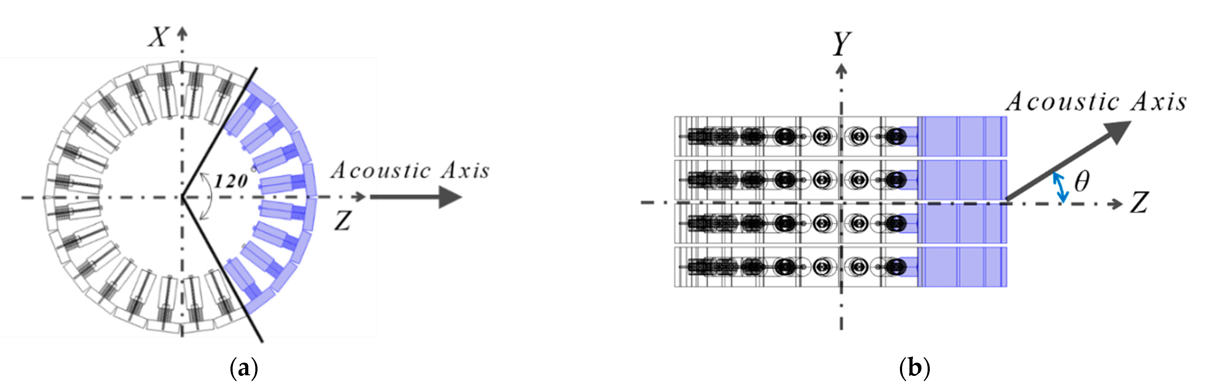
3.1. Analysis Model

The results of a general-purpose package (Multiphysics FEM software) were compared with the results obtained by the proposed method for a model with surrounding structures to confirm the validity of the proposed method.

The analysis model is a cylindrical array of 96 piston transducers arranged in 24 staves surrounded by an acoustic window, as shown in Figure 4. Figure 4a shows the geometry, and Figure 4b shows a FE-BE coupling model used in the proposed method to obtain the acoustic radiation impedance, $Z_{r,ik}$, and the transfer matrix $H$. In Figure 4b, only the ellipsoid-shaped acoustic window is the structural finite element, the fluid 1 between the array and the acoustic window and the fluid 2 outside the acoustic window are the boundary elements. The input boundary condition of the FE-BE coupling analysis is shown in Equation (28). The acoustic radiation impedance, $Z_{r,ik}$, can be obtained by postprocessing the analyzed surface sound pressure result as Equation (29). Although the transfer matrix $H$ can be obtained using Equation (35), it is often difficult to access the system matrices (e.g., $M$, $C$, $K$, $A_1$, $B_1$, $A_2$ and $B_2$) of the general-purpose package. In that case, it can be obtained by setting the input boundary condition as Equation (28) and postprocessing the sound pressure result in the point of interest field. For example, the kth column of the transfer matrix $H$ can be obtained by setting the input boundary condition as Equation (28). Figure 4c shows the conventional FE model. In the conventional FE model, an open boundary condition, such as perfectly matched layer (PML), is given to the surface of the sphere that is the external fluid domain. Moreover, each transducer is given a boundary condition that allows it to move in only piston mode without rocking mode because the transducer is designed so that the rocking mode does not occur.

Figure 5a shows the tonpilz transducer used in the array, and Figure 5b shows the transducer FE model used for the conventional analytical method. The material of the piezo-stack is PZT-4, and that of the tail and stress rod is AISI 4340 steel. The density of the head is 2700 ${[\mathrm{kg} \mathrm{m}}^{-3}]$. The material properties and dimensions of the analytical model are given in

Table 1. Material properties of the analysis model.

Component	Property	Symbol	Value
Piston Head (Rigid)	Density	$\rho$	2700 [kg/m3]
PZT Ceramic (PZT-4)	Compliance coefficient	$s_{33}^E$	1.55 × 10−11 [1/Pa]
		$s_{11}^E$	1.23 × 10−11 [1/Pa]
		$s_{12}^E$	−4.05 × 10−12 [1/Pa]
		$s_{13}^E$	−5.31 × 10−12 [1/Pa]
		$s_{44}^E$	3.90 × 10−11 [1/Pa]
	Piezoelectric coefficient	$d_{33}^{}$	2.89 × 10−10 [C/N]
		$d_{31}^{}$	−1.23 × 10−10 [C/N]
		$d_{15}^{}$	4.96 × 10−10 [C/N]
	Relative permittivity coefficient	${\epsilon }_{33}^T/{\epsilon }_0^{}$	1300
		${\epsilon }_{11}^T/{\epsilon }_0^{}$	1475
	Density	$\rho$	7500 [kg/m3]
Tail Mass & Stress Rod (Steel AISI 4340)	Density	$\rho$	7850 [kg/m3]
	Young’s Modulus	$E$	205 × 109 [Pa]
	Poisson’s Ratio	$\upsilon$	0.28
Acoustic Window	Density	$\rho$	1500 [kg/m3]
	Longitudinal wave speed	$C_P^{}$	2400 [m/s]
	Shear wave speed	$C_S^{}$	1230 [m/s]

and

Table 2. Dimensions of the analysis model.

Component	Dimensions	Symbol	Value
Piston Head	Cross-sectional area	$A_{\mathrm{Head}}$	0.04 [m2]
	Longitudinal length	$L_{\mathrm{Head}}$	0.06 [m]
PZT Ceramic	Cross-sectional area	$A_{\mathrm{PZT}}^{}$	3.77 × 10−3 [m2]
	Longitudinal length	$L_{\mathrm{PZT}}$	0.08 [m]
	Number of rings	$n_{\mathrm{PZT}}$	10
	Thickness of each ring	$t_{\mathrm{PZT}}$	8.00 × 10−3 [m]
Tail Mass	Cross-sectional area	$A_{\mathrm{Tail}}$	7.12 × 10−3 [m2]
	Longitudinal length	$L_{\mathrm{Tail}}$	0.192 [m]
Stress Rod	Cross-sectional area	$A_{\mathrm{st}}$	7.80 × 10−5 [m2]
	Longitudinal length	$L_{\mathrm{st}}$	0.272 [m]
Array	Height	$H_{array}$	0.88 [m]
	Diameter	$D_{array}$	1.68 [m]
Acoustic Window	Thickness	$t_{window}$	0.025 [m]
		$a_{window}$	1.25 [m]
	half-length of the principal axes	$b_{window}$	1.25 [m]
		$c_{window}$	0.75 [m]

, respectively. The spacing between transducers is set to tenths of “the length of one side of the square transducer head surface”.

3.2. Analysis Condition

This section describes how to determine the input vector $F_i$ of the impedance matrix equation. It is assumed that no external forces are applied to the array as the example analysis model is a projector array. The conditions are expressed by Equation (36).

$$\begin{array}{l}{F}_{1,i}=0\hspace{0.17em}\\ F_{2,i}=0\hspace{0.17em}\hspace{0.17em}\hspace{0.17em}\hspace{0.17em}\hspace{0.17em}\hspace{0.17em}\hspace{0.17em}\hspace{0.17em}\hspace{0.17em}\hspace{0.17em}\hspace{0.17em}\hspace{0.17em}\hspace{0.17em}\hspace{0.17em}\hspace{0.17em}where\hspace{0.17em}\hspace{0.17em}\hspace{0.17em}\hspace{0.17em}i=1,\cdots ,96\\ F_{3,i}=0\hspace{0.17em}\end{array}$$

(36)

Phase shifting the applied voltages is done to steer a projected beam. Normally, about 120° of the cylindrical surfaces is used for beam steering [36]. Thus, only 8 of the 24 staves are used in this model, which means that 32 of 96 transducers are operated, as shown in Figure 6.

The phase shifts must be proportional to the perpendicular distance from each transducer to the plane. The beam can also be steered in the elevation angle $\theta$ by phase shifting. The applied voltage of each transducer has the phase shown in Equation (37).

$$\begin{array}{l}{V}_i=\sqrt{2}{V}_{rms}^{}{\mathrm{e}}^{\mathrm{j}k{d}_i}\hspace{0.17em}\hspace{0.17em}[\mathrm{V}]\hspace{0.17em}\hspace{0.17em}\hspace{0.17em}\hspace{0.17em}\hspace{0.17em}\hspace{0.17em}\hspace{0.17em}\hspace{0.17em}\hspace{0.17em}\hspace{0.17em}\hspace{0.17em}\hspace{0.17em}\hspace{0.17em}where\hspace{0.17em}\hspace{0.17em}i=1,\cdots ,32\\ V_i=0\hspace{0.17em}\hspace{0.17em}[\mathrm{V}]\hspace{0.17em}\hspace{0.17em}\hspace{0.17em}\hspace{0.17em}\hspace{0.17em}\hspace{0.17em}\hspace{0.17em}\hspace{0.17em}\hspace{0.17em}\hspace{0.17em}\hspace{0.17em}\hspace{0.17em}\hspace{0.17em}\hspace{0.17em}\hspace{0.17em}\hspace{0.17em}\hspace{0.17em}\hspace{0.17em}\hspace{0.17em}\hspace{0.17em}\hspace{0.17em}\hspace{0.17em}\hspace{0.17em}\hspace{0.17em}\hspace{0.17em}where\hspace{0.17em}\hspace{0.17em}i=33,\cdots ,96\end{array}$$

(37)

where $d_i$ is the perpendicular distance from each transducer to the plane, and $V_{rms}^{}$ is the RMS value of the applied voltage.

By changing the Equation (19) as following equation, and fill the input force vector, ${\left[\begin{array}{ccc}{F}_1& \cdots & F_n\end{array}\right]}^{\mathrm{T}}$, with Equations (36) and (37), the responses of the array can be obtained from the output vector, ${\left[\begin{array}{ccc}{u}_1& \cdots & u_n\end{array}\right]}^{\mathrm{T}}$.

$$\left\{\begin{array}{c}{u}_1\\ ⋮\\ u_n\end{array}\right\}={\left[\begin{array}{ccc}{\tilde{Z}}_{11}& \cdots & {\tilde{Z}}_{1n}\\ ⋮& \ddots & ⋮\\ {\tilde{Z}}_{n1}& \cdots & {\tilde{Z}}_{nn}\end{array}\right]}^{-1}\left\{\begin{array}{c}{F}_1\\ ⋮\\ F_n\end{array}\right\}\hspace{0.17em}\hspace{0.17em}$$

(38)

3.3. Analysis Result

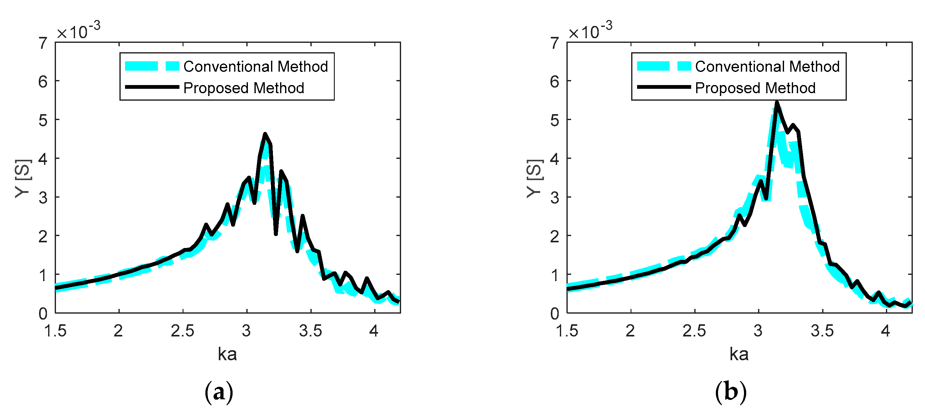
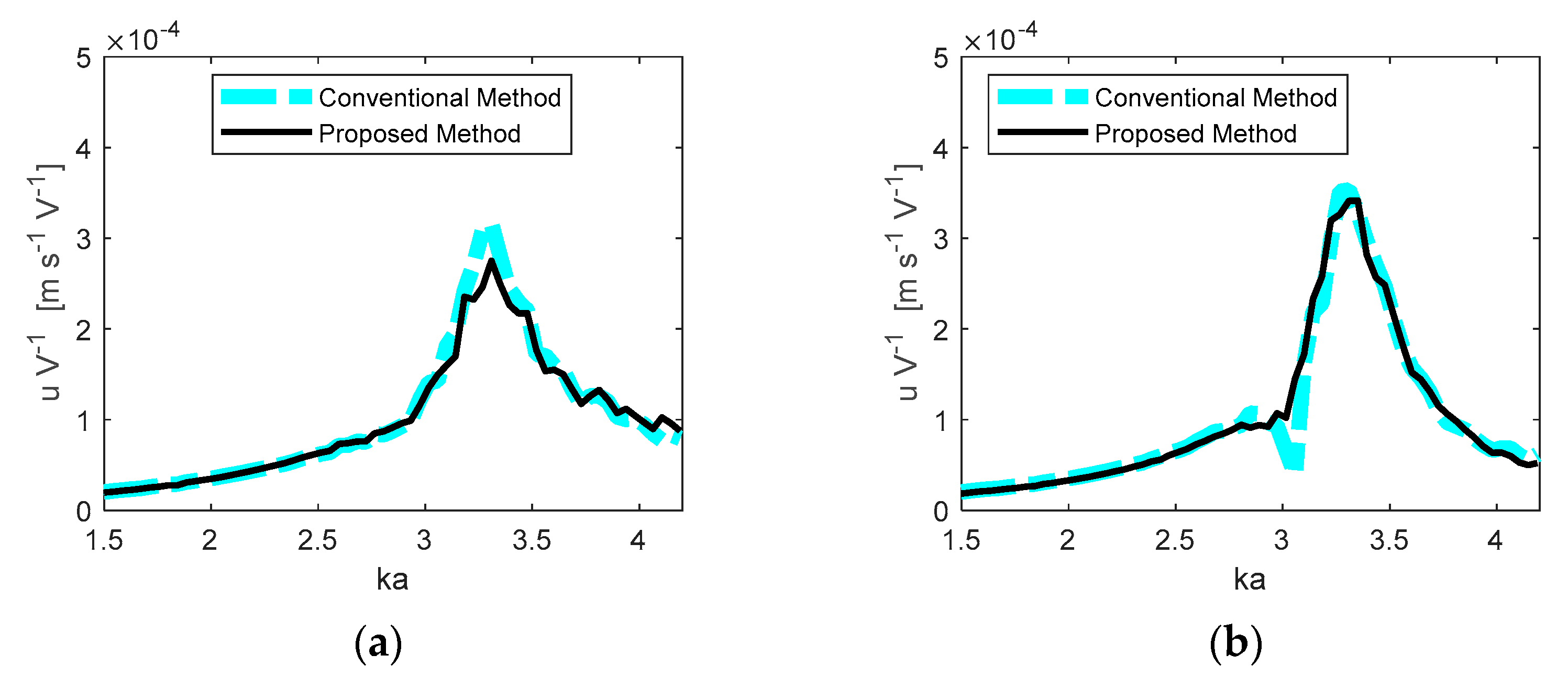
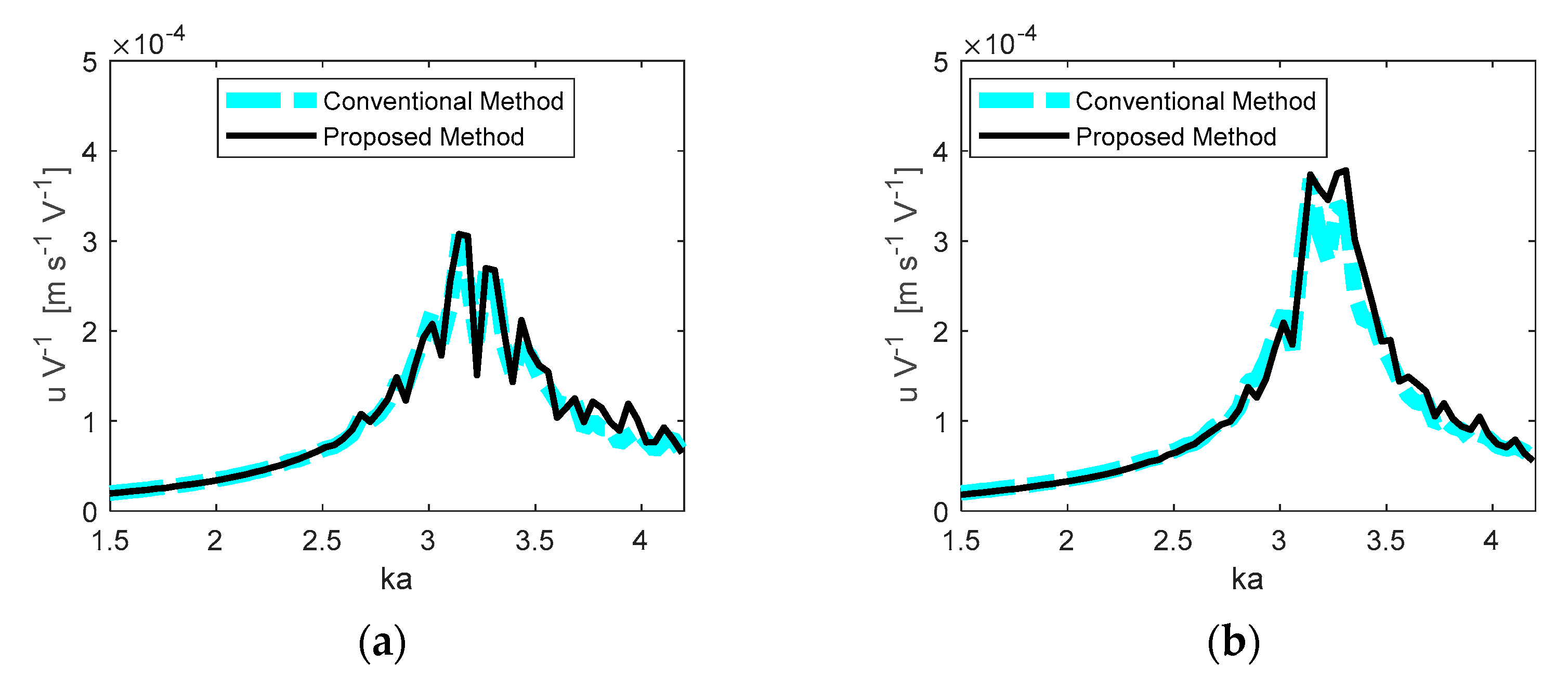
3.3.1. Response of Each Transducer

This section presents the electrical current and the vibration velocity obtained from the impedance matrix equation in the form of a transfer function for the applied voltage. The results are compared to the FE analysis results. The 32 operated transducers and their numbers are shown in Figure 7. Each operating transducer has a unique transfer function depending on its position and the direction of the projected beam.

Figure 8, Figure 9, Figure 10 and Figure 11 show the resulting electrical and mechanical transfer functions for randomly selected transducers #7 and #9. In each graph, the x-axis is the normalized frequency, $ka$, for the size of the transducer, where $a$ is the length of one side of the radiating surface of the head (0.2 m in this case). The amplitudes of the electrical admittances of transducers #7 and #9 are shown in Figure 8 and Figure 9, respectively. The amplitudes of the transfer function between the applied voltage and the head velocities of transducers #7 and #9 are shown in Figure 10 and Figure 11, respectively. Graphs are shown for elevation angles of the projected beam of 0° and 30°. Here, the analyzed frequency range is approximately $ka=1.5~4.2$.

The conventional FEM results and the results of the proposed method match well. The validity of the proposed method can be confirmed by the fact that the transfer functions of each transducer obtained by the two methods are very similar. In Figure 8, Figure 9, Figure 10 and Figure 11, the analysis results are rather complex. This occurs because the sound diffraction, transmission, and vibration mode of the acoustic window have complex effects on the acoustic field produced by the sonar (the crosstalk phenomenon).

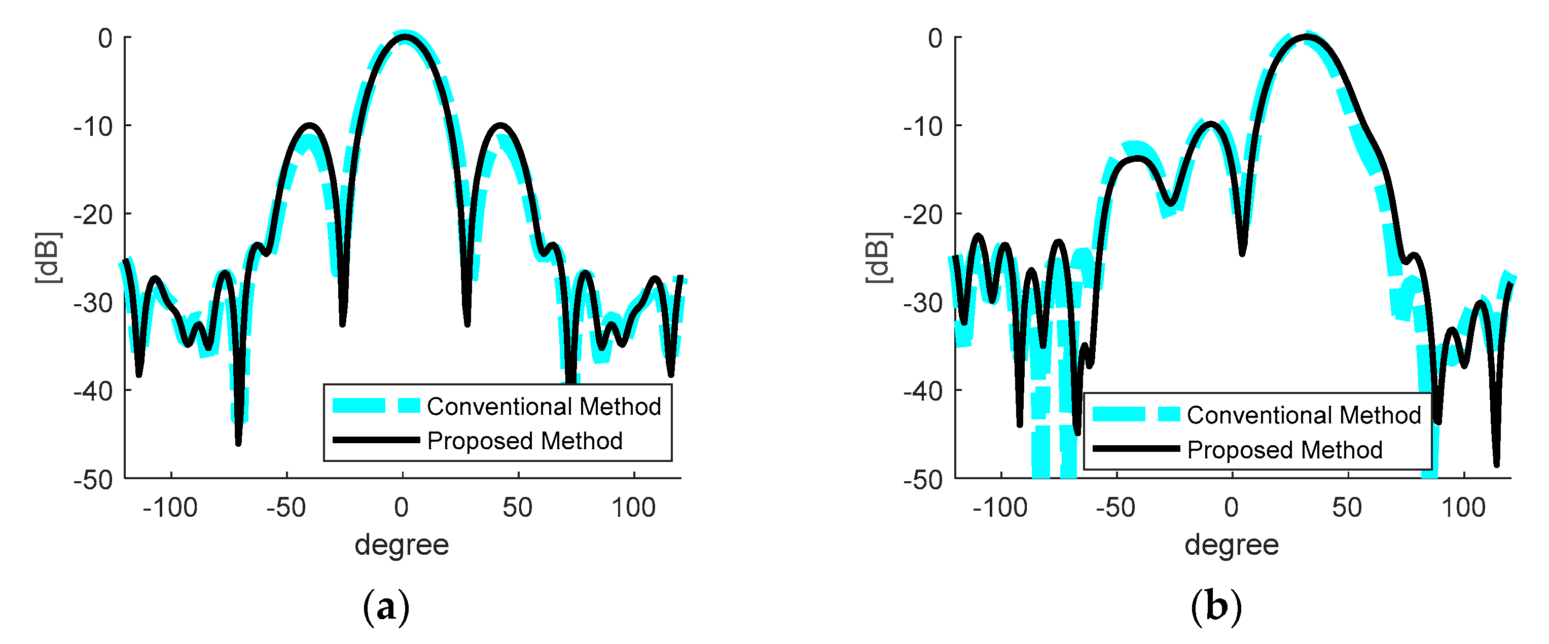
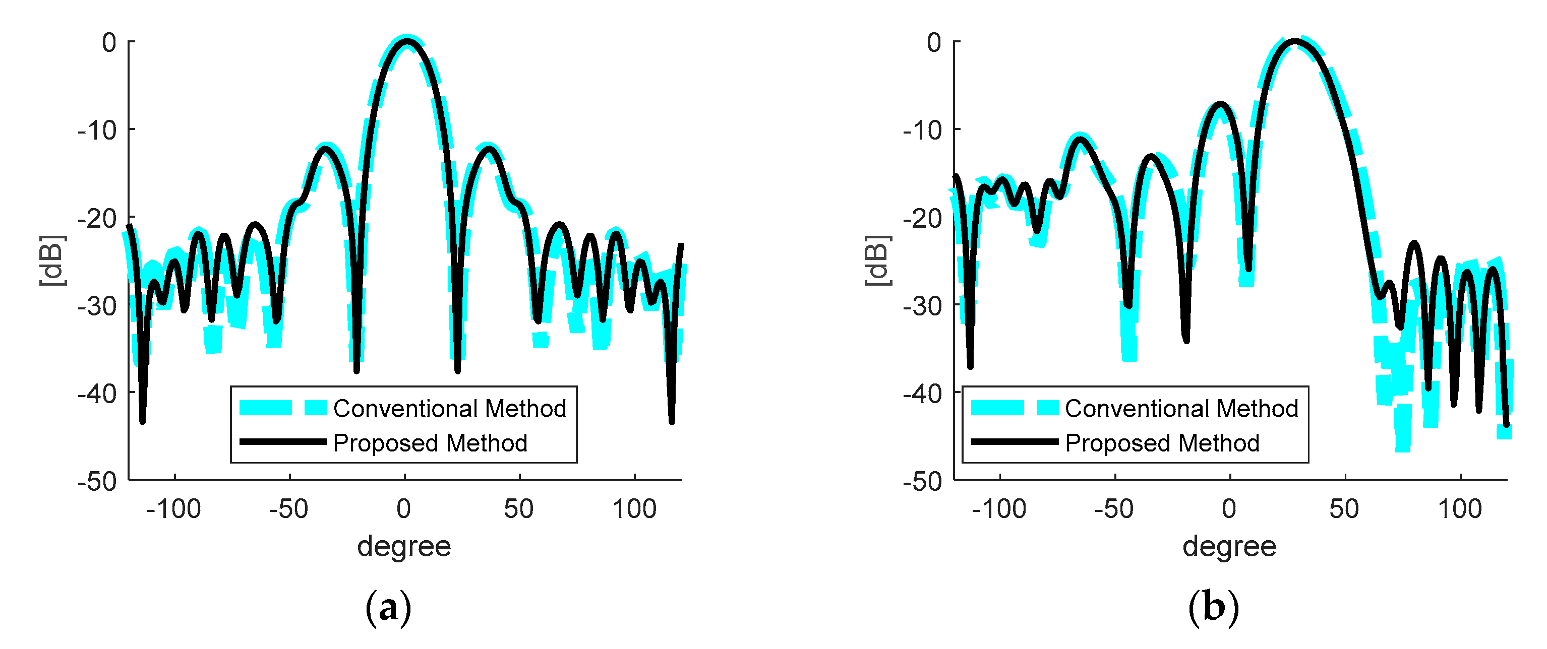
3.3.2. Array Performance

In this section, the beam pattern and TVR results calculated by the proposed method are compared with the conventional FEM results. The beam pattern and TVR are obtained by postprocessing the pressure at the field point of the far field. In this example, as the sound field at a distance of 100 m from the array has sufficiently developed into the far field, the field points are placed on a circle with a radius of 100 [m] on the y-z plane as shown in the Figure 12. TVR is defined as

$$TVR=20\log \left[\frac{P_{rms}\left(r\right)}{P_{ref}}\frac{r}{V_{rms}}\right]\hspace{0.17em}\hspace{0.17em}\hspace{0.17em}\hspace{0.17em}\hspace{0.17em}\hspace{0.17em}\hspace{0.17em}\hspace{0.17em}\hspace{0.17em}\hspace{0.17em}\hspace{0.17em}\hspace{0.17em}\hspace{0.17em}\hspace{0.17em}\hspace{0.17em}\hspace{0.17em}\hspace{0.17em}\hspace{0.17em}\hspace{0.17em}\hspace{0.17em}where\hspace{0.17em}\hspace{0.17em}\hspace{0.17em}{P}_{ref}=1\left[\mu Pa\right]$$

(39)

where $P_{rms}\left(r\right)$ is the rms sound pressure measured at a distance $r$ from the source along the acoustic axis. Here, $r$ is multiplied to $P_{rms}\left(r\right)$ as TVR is normalized over distance $r$.

The resulting TVR is shown in Figure 13. Results are shown for elevation angles of the projected beam of 0° and 30°. Typically, the operating frequency band of the array is designed as the frequency band near the maximum peak of the TVR. As shown in Figure 13, the maximum peak of TVR occurs between about $ka=3.0$ and $ka=3.5$, so the resulting beam patterns at $ka=3.0$ and $ka=3.5$ are shown in Figure 14 and Figure 15, respectively.

The validity of the proposed method confirms that the array performances obtained by the two methods match. These analysis results for the exterior acoustic field are rather complex. In particular, the TVR results have several small peaks as shown in Figure 13. This occurs because the sound diffraction, transmission, and vibration mode of the acoustic window have a complex effect on the acoustic field produced by the transducer array (the crosstalk phenomenon).

3.4. Evaluation of Numerical Performance (in Terms of DOFs Reduction)

This section describes the numerical performance of the proposed method in terms of DOFs reduction. For numerical models such as FE model or FE-BE coupling model, DOFs is the number of unknown variables of the matrix equation for calculating the dynamic behavior of a physical system. The higher the DOFs, the greater the computational effort. Therefore, from the reduction rate of DOFs, we evaluated how high numerical performance the method proposed in this study has compared to the conventional full FEM.

We modeled cylindrical arrays as shown Figure 4a and configured four different sets of row and stave numbers, N_C and N_R to consider various sizes of problems: N_C = 24 and N_R = 4; N_C = 36 and N_R = 6; N_C = 48 and N_R = 8; and N_C = 60 and N_R = 10. We also considered four different analysis frequencies represented by ka: ka = 2, 3, 4, and 5. The following are basic schemes for generating the FE-BE coupling model for the proposed method and the FE model for the conventional method:

• The size of one side of the acoustic element is set to about $\lambda /8$ [37].
• The FE of the structure should be generated so that the mode shapes that are within 2 times the maximum analysis frequency can be well represented.
• The shape of the acoustic window is assumed to be an oblate spheroid, and its size is set to increase in proportion to the array size. Here, the sizes of the half-length of the principal axes are assumed to be $a_{window}=\hspace{0.17em}1.5R_{Array}$ and $c_{window}=1.7N_R\left(a+d\right)/2$. $R_{Array}$ is the radius of the array.
• For the conventional full FEM, an adequate amount of space is required between the array and the outer surface in order to apply an open boundary condition to the surface of the acoustic region. The free space of the open boundary is assumed to be set to 300% of the size of the structure. Thus, the radius of the open boundary is three times the half-length of the principal axes.

The DOFs for the two models (FE-BE coupling model and the conventional FE model) were obtained using the general-purpose software’s DOF calculation function. The DOFs required for a reliable solution are summarized in

Table 3. Degrees of freedom (DOFs) of the FE-BE coupling model and full FE model.

	ka = 2.0		ka = 3.0		ka = 4.0		ka = 5.0
Array Size	$\mathit{D}\mathit{O}{\mathit{F}}_{\mathit{F}\mathit{E}-\mathit{B}\mathit{E}}$	$\mathit{D}\mathit{O}{\mathit{F}}_{\mathit{F}\mathit{u}\mathit{l}\mathit{l}\mathit{F}\mathit{E}}$	$\mathit{D}\mathit{O}{\mathit{F}}_{\mathit{F}\mathit{E}-\mathit{B}\mathit{E}}$	$\mathit{D}\mathit{O}{\mathit{F}}_{\mathit{F}\mathit{u}\mathit{l}\mathit{l}\mathit{F}\mathit{E}}$	$\mathit{D}\mathit{O}{\mathit{F}}_{\mathit{F}\mathit{E}-\mathit{B}\mathit{E}}$	$\mathit{D}\mathit{O}{\mathit{F}}_{\mathit{F}\mathit{u}\mathit{l}\mathit{l}\mathit{F}\mathit{E}}$	$\mathit{D}\mathit{O}{\mathit{F}}_{\mathit{F}\mathit{E}-\mathit{B}\mathit{E}}$	$\mathit{D}\mathit{O}{\mathit{F}}_{\mathit{F}\mathit{u}\mathit{l}\mathit{l}\mathit{F}\mathit{E}}$
NC = 24, NR = 4	$0.5576 \times$105	$0.1943 \times$107	$1.232 \times$105	$0.5055 \times$107	$2.197 \times$105	$1.109 \times$107	$3.408 \times$105	$2.102 \times$107
NC = 36, NR = 6	$1.251 \times$105	$0.5805 \times$107	$2.763 \times$105	$1.621 \times$107	$4.931 \times$105	$3.642 \times$107	$7.648 \times$105	$6.968 \times$107
NC = 48, NR = 8	$2.220 \times$105	$1.287 \times$107	$4.907 \times$105	$3.744 \times$107	$8.757 \times$105	$8.517 \times$107	$13.58 \times$105	$16.38 \times$107
NC = 60, NR = 10	$3.467 \times$105	$2.411 \times$107	$7.664 \times$105	$7.198 \times$107	$13.68 \times$105	$16.51 \times$107	$21.22 \times$105	$31.84 \times$107

. The DOFs of the proposed method are denoted by $DO{F}_{FE-BE}$, and that of the conventional full FEM are denoted by $DO{F}_{FullFE}$.

$DO{F}_{FullFE}/DO{F}_{FE-BE}$ is an indicator of how many times the DOFs have been reduced when using the proposed hybrid method. Figure 16 shows the ratio of DOFs of the proposed method to the conventional method. The dashed-dotted line, the dotted line, the broken line, and the solid line represent the cases of the transducer arrays corresponding to “N_C = 24 and N_R = 4”, “N_C = 36 and N_R = 6”, “N_C = 48 and N_R = 8”, and “N_C = 60 and N_R = 10”, respectively. As shown in Figure 16, higher frequency and a larger size of the array result in higher values of $DO{F}_{FullFE}/DO{F}_{FE-BE}$.

4. Conclusions

This study developed a hybrid modeling method for an effective analysis of an acoustic transducer array with arbitrarily shaped flexible surrounding structures. More precisely, the proposed analysis procedure is divided into two parts: The first part is for the construction of the impedance matrix using an EC model and a FE-BE coupling model. We derived the electro-mechanical-acoustic coupling impedance matrix equation and established the procedure of calculation of the impedance matrices. Specifically, the mechanical and electrical impedances were derived from the LPM and T-network, a type of the EC model. The acoustic radiation impedances were calculated from the FE-BE coupling model, which represented the surrounding structure and acoustic coupling. The second part is dedicated to the construction of the acoustic transfer matrix using the FE-BE coupling method. Here, the acoustic pressure on each head surface can be calculated using the acoustic radiation impedance and the head velocities. The far-field acoustic pressure can be also evaluated by the acoustic transfer matrix equation and the head velocities.

The proposed method was applied to sonar with 96 tonpliz transducers and surrounding structures. The response of each transducer was calculated (such as the electrical admittance and the vibration velocity) along with the array performance (such as the far-field directivity pattern and the TVR). The results were compared with the results of FEM software. The results showed good agreement. To evaluate the numerical performance of the proposed method, the DOFs of the FE-BE models and the full FE model were investigated and compared. The DOF reduction rate of the proposed method to the conventional FEM is increased as the analysis frequency, array size, or size of the surrounding structures increased.

The main conclusion is that this proposed hybrid method can be used to effectively estimate the performance of the array while taking into account the surrounding structure and acoustic medium coupling. The computational effort is significantly reduced with the equivalent accuracy to the conventional FE analysis. Therefore, the proposed method is expected to be useful for conceptual design that require frequent design changes.

References

- Rizwan, M.K.; Laureti, S.; Mooshofer, H.; Goldammer, M.; Ricci, M. Ultrasonic Imaging of Thick Carbon Fiber Reinforced Polymers through Pulse-Compression-Based Phased Array. Appl. Sci. 2021, 11, 1508. [Google Scholar] [CrossRef]
- Peralta, L.; Ramalli, A.; Reinwald, M.; Eckersley, R.J.; Hajnal, J.V. Impact of Aperture, Depth, and Acoustic Clutter on the Performance of Coherent Multi-Transducer Ultrasound Imaging. Appl. Sci. 2020, 10, 7655. [Google Scholar] [CrossRef] [PubMed]
- Angerer, M.; Zapf, M.; Leyrer, B.; Ruiter, N.V. Model-Guided Manufacturing of Transducer Arrays Based on Single-Fibre Piezocomposites. Appl. Sci. 2020, 10, 4927. [Google Scholar] [CrossRef]
- Go, D.; Kang, J.; Song, I.; Yoo, Y. Efficient Transmit Delay Calculation in Ultrasound Coherent Plane-Wave Compound Imaging for Curved Array Transducers. Appl. Sci. 2019, 9, 2752. [Google Scholar] [CrossRef] [Green Version]
- Bae, S.; Song, T.-K. Methods for Grating Lobe Suppression in Ultrasound Plane Wave Imaging. Appl. Sci. 2018, 8, 1881. [Google Scholar] [CrossRef] [Green Version]
- Mestouri, H.; Loussert, A.; Keryer, G. Finite Element Modeling of 2-D Transducer Arrays. J. Acoust. Soc. Am. 2008, 123, 3116. [Google Scholar] [CrossRef]
- Yamamoto, M.; Inoue, T.; Shiba, H.; Kitamura, Y. Finite-Element Method Analysis of Low-Frequency Wideband Array Composed of Disk Bender Transducers with Differential Connections. Jpn. J. Appl. Phys. 2009, 48, 07GL06. [Google Scholar] [CrossRef]
- Tilmans, H.A. Equivalent circuit representation of electromechanical transducers: I. Lumped-parameter systems. J. Micromech. Microeng. 1996, 6, 157–176. [Google Scholar] [CrossRef]
- Tilmans, H.A. Equivalent circuit representation of electromechanical transducers: II. Distributed-parameter systems. J. Micromech. Microeng. 1997, 7, 285–309. [Google Scholar] [CrossRef]
- Lee, J.; Seo, I.; Han, S.M. Radiation power estimation for sonar transducer arrays considering acoustic interaction. Sens. Actuator A Phys. 2001, 90, 1–6. [Google Scholar] [CrossRef]
- Oguz, H.K.; Atalar, A.; Köymen, H. Equivalent circuit-based analysis of CMUT cell dynamics in arrays. IEEE Trans. Ultrason. Ferroelectr. Freq. Control. 2013, 60, 1016–1024. [Google Scholar] [CrossRef] [PubMed]
- Hwang, Y.; Moon, W.; Je, Y.; Kim, W.; Lee, S. A Precise Equivalent-Circuit Model for a Circular Plate Radiator. Acta Acust. United Acust. 2018, 104, 79–86. [Google Scholar] [CrossRef]
- Audoly, C. Some aspects of acoustic interactions in sonar transducer arrays. J. Acoust. Soc. Am. 1991, 89, 1428–1433. [Google Scholar] [CrossRef]
- Yokoyama, T.; Henmi, M.; Hasegawa, A.; Kikuchi, T. Effects of mutual interactions on a phased transducer array. Jpn. J. Appl. Phys. 1998, 37, 3166–3171. [Google Scholar] [CrossRef]
- Meynier, C.; Teston, F.; Certon, D. A multiscale model for array of capacitive micromachined ultrasonic transducers. J. Acoust. Soc. Am. 2010, 128, 2549–2561. [Google Scholar] [CrossRef]
- Rudgers, A.J. A correlation technique for determining the self-and mutual-radiation impedances of transducers in an array. J. Acoust. Soc. Am. 1974, 55, 759–765. [Google Scholar] [CrossRef]
- Sherman, C.H.; Butler, J.L. Chapter 7. Transducer Models. In Transducers and Arrays for Underwater Sound, 4th ed.; Springer: New York, NY, USA, 2007; pp. 338–350. [Google Scholar]
- Klapman, S.J. Interaction impedance of a system of circular pistons. J. Acoust. Soc. Am. 1940, 11, 289–295. [Google Scholar] [CrossRef]
- Robey, D.H. On the radiation impedance of an array of finite cylinders. J. Acoust. Soc. Am. 1955, 27, 706–710. [Google Scholar] [CrossRef]
- Sherman, C.H. Mutual radiation impedance of sources on a sphere. J. Acoust. Soc. Am. 1959, 31, s947–s952. [Google Scholar] [CrossRef]
- Pritchard, R.L. Mutual acoustic impedance between radiators in an infinite rigid plane. J. Acoust. Soc. Am. 1960, 32, 730–737. [Google Scholar] [CrossRef]
- Greenspon, J.E.; Sherman, C.H. Mutual-Radiation Impedance and Nearfield Pressure for Pistons on a Cylinder. J. Acoust. Soc. Am. 1964, 36, 149–153. [Google Scholar] [CrossRef]
- Arase, E.M. Mutual radiation impedance of square and rectangular pistons in a rigid infinite baffle. J. Acoust. Soc. Am. 1964, 36, 1521–1525. [Google Scholar] [CrossRef]
- Mangulis, V. Nearfield Pressure for an Infinite Phased Array of Circular Pistons. J. Acoust. Soc. Am. 1967, 41, 412–418. [Google Scholar] [CrossRef]
- Schenck, H.A. Improved integral formulation for acoustic radiation problems. J. Acoust. Soc. Am. 1968, 44, 41–58. [Google Scholar] [CrossRef]
- Thompson, W., Jr. The computation of self-and mutual-radiation impedances for annular and elliptical pistons using Bouwkamp’s integral. J. Sound Vib. 1971, 17, 221–233. [Google Scholar] [CrossRef]
- Stepanishen, P.R. The radiation impedance of a rectangular piston. J. Sound Vib. 1977, 55, 275–288. [Google Scholar] [CrossRef]
- Lee, J.; Seo, I. Radiation impedance computations of a square piston in a rigid infinite baffle. J. Sound Vib. 1996, 198, 299–312.a. [Google Scholar] [CrossRef]
- Rdzanek, W.; Rdzanek, W.; Różycka, A. The Green function for the Neumann boundary value problem at the semiinfinite cylinder and the flat infinite baffle. Arch. Acoust. 2014, 32, 7–12. [Google Scholar]
- Rdzanek, W.P.; Rdzanek, W.J.; Pieczonka, D. The acoustic impedance of a vibrating annular piston located on a flat rigid baffle around a semi-infinite circular rigid cylinder. Arch. Acoust. 2012, 37, 411–422. [Google Scholar] [CrossRef] [Green Version]
- Pyo, S.; Roh, Y. Analysis of the crosstalk in an underwater planar array transducer by the equivalent circuit method. Jpn. J. Appl. Phys. 2017, 56, 07JG01-1–07JG01-6. [Google Scholar]
- Costabel, M. Symmetric methods for the coupling of finite elements and boundary elements (invited contribution). In Mathematical and Computational Aspects, 3rd ed.; Springer: Berlin/Heidelberg, Germany, 1987; pp. 411–420. [Google Scholar]
- Amini, S.; Harris, P.J.; Wilton, D.T. Coupled Boundary and Finite Element Methods for the Solution of the Dynamic Fluid-Structure Interaction Problem; Springer Science & Business Media: Berlin/Heidelberg, Germany, 2012. [Google Scholar]
- Hong, C.S.; Shin, K.K. Applications of General-purpose Packages for Fluid-structure Interaction Problems. Trans. Korean Soc. Noise Vib. Eng. 1997, 7, 571–578. [Google Scholar]
- Atalla, N.; Sgard, F. Chapter 8. Problem of exterior coupling. In Finite Element and Boundary Methods in Structural Acoustics and Vibration; CRC Press: Boca Raton, FL, USA, 2015. [Google Scholar]
- Sherman, C.H.; Butler, J.L. Chapter 5. Projector Arrays. In Transducers and Arrays for Underwater Sound, 4th ed.; Springer: New York, NY, USA, 2007; pp. 223–228. [Google Scholar]
- Marburg, S. Six boundary elements per wavelength: Is that enough? J. Comput. Acoust. 2002, 10, 25–51. [Google Scholar] [CrossRef]