
Experimental Determination of Lamb-Wave Attenuation Coefficients


Department of Materials Science and Engineering, University of California, Los Angeles (UCLA), Los Angeles, CA 90095, USA
Appl. Sci. 2022, 12(13), 6735; https://doi.org/10.3390/app12136735
Submission received: 14 June 2022
/
Revised: 26 June 2022
/
Accepted: 28 June 2022
/
Published: 2 July 2022
(This article belongs to the Special Issue Elastic Waves and Acoustic Emission for Innovative Monitoring of Structures and Engineering Systems)
Abstract
:This work determined the attenuation coefficients of Lamb waves of ten engineering materials and compared the results with calculated Lamb-wave attenuation coefficients, α–S and α–A. The Disperse program and a parametric method based on Disperse results were used for calculations. Bulk-wave attenuation coefficients, αL and αT, were required as input parameters to the Disperse calculations. The calculated α–S and α–A values were found to be dominated by the αT contribution. Often α–Ao coincided with αT. The values of αL and αT were previously obtained or newly measured. Attenuation measurement relied on Lamb-wave generation by pulsed excitation of ultrasonic transducers and on surface-displacement detection with point contact receivers. The frequency used ranged from 10 kHz to 1 MHz. A total of 14 sheet and plate samples were evaluated. Sample materials ranged from steel, Al, and silicate glass with low attenuation to polymers and a fiber composite with much higher attenuation. Experimentally obtained Lamb-wave attenuation coefficients, α–S and α–A, for symmetric and asymmetric modes, were mostly for the zeroth mode. Plots of α–So and α–Ao values against frequency were found to coincide reasonably well to theoretically calculated curves. This study confirmed that the Disperse program predicts Lamb-wave attenuation coefficients for elastically isotropic materials within the limitation of the contact ultrasonic techniques used. Further refinements in experimental methods are needed, as large deviations often occurred, especially at low and high frequencies. Methods of refinement are suggested. Displacement measurements were quantified using Rayleigh wave calibration. For signals below 300 kHz, 1-mV receiver output corresponded to 1-pm displacement. Peak displacements after 200-mm propagation were found to range from 10 pm to 1.5 nm. With the use of signal averaging, the point-contact sensor was capable of detecting 1-pm displacement with 40 dB signal-to-noise ratio and had equivalent noise of 4.3 fm/√Hz. Approximate expressions for α–So and α–Ao were obtained, and an empirical correlation was found between bulk-wave attenuation coefficients, i.e., αT = 2.79 αL, for over 150 materials.
1. Introduction
For more than half a century, ultrasonic testing (UT) and acoustic emission (AE) have played key roles in the field of nondestructive evaluation (NDE) [1,2], and more recently contributed substantially to the successful development of structural health monitoring (SHM) [3]. Among the methods that are based on elastic wave propagation, those using guided waves (GW), e.g., Lamb and Rayleigh waves, have made significant advances in recent decades, benefitting from improved computational mechanics, signal generation and sensing methods, and signal processing techniques [4,5,6]. Two reviews provided detailed mathematical developments on guided waves from Lord Rayleigh’s works to the present, covering more than a century [7,8].
The first successful NDE application of guided waves occurred at Aerojet for the AE inspection of Polaris missile chambers in the early 1960s [9], followed by many more AE tests of rocket motorcases. Soon after, AE inspection was expanded to various pressurized installations, including pipelines, tanks, vessels, etc., of both metals and fiber-reinforced composites [2]. In 1967, buried pipelines were inspected using 300-m sensor spacing and detected corrosion pits at 100-mm location accuracy [2] (p. 166). By the 1980s, many industrial tanks and vessels in the USA were regularly inspected under the ASME Boiler and Pressure Vessels Codes and ASTM standards [10]. These AE tests were, however, conducted without benefiting from the theories of GW propagation, since field measurements of wave propagation velocities were successfully incorporated into the test routines. Up to 1990, only three AE papers were found to use the Lamb wave dispersion curves. Two were for detection frequency selection by Hutton [11] and Graham and Alers [12]. The third was on long distance pipeline AE inspection by Pollock [13]. The GW attenuation was measured on long pipelines of up to 300 m [2,13], and the Pollock results at 30 kHz were analyzed in [14], separating signal reduction into geometrical spreading and steel absorption components. The GW attenuation was very small, or 0.17 dB/m, demonstrating the benefit of GW utilization on pipelines. In 1991, Gorman introduced mode-dependent velocities of GW, specifically Lamb waves, to properly conduct AE source location in thin structures [15]. In the 1990s, numerous computational studies started to make GW properties more accessible, even for anisotropic materials. A series of studies by Hamstad and coworkers [16] used three-dimensional, dynamic finite element modeling and correlated source motion to displacements at sensor positions, accounting for GW propagation effects through a plate. These studies have been extended to fiber-reinforced composites [6]. GW-based AE studies (or GWAE) also profited from wavelet analysis as mode separation with time and frequency was visualized. Takemoto and coworkers [17] developed wavelet analysis software based on Gabor wavelets and made available the source code written by Hayashi, Y. This code was implemented by Vallen, J. in 2003 into an easy-to-use free software, AGU-Vallen Wavelet [18]. With continual support of Vallen Systeme (Wolfratshausen, Germany), this wavelet software has assisted GW studies and NDE engineers everywhere.
Viktorov gathered main results of early studies of Lamb and Rayleigh waves [19]. In addition to velocity dispersion curves, parametric equations of attenuation of Lamb and Rayleigh waves were given. Around 1970, the GW dispersion curves of only a few materials (including Al, steel, and polymethyl methacrylate (PMMA)) were commonly accessible [20,21]. In the following 50 years, GW mechanics and NDE based on GW ultrasonic testing (or GWUT) have been refined, passing many milestones. Long-range inspection of pipelines has been practiced for two decades [22,23,24]. GW dispersion analysis software packages became available for GW velocities and attenuation [25,26,27]. GW analysis methods for anisotropic materials and structures were developed [4,28,29,30,31,32,33,34,35,36], and GW in non-linear solids started to provide a new NDE approach, especially for detecting fatigue damage [37,38,39]. The uses of laser devices enabled, for example, detailed evaluation of composite damages and GW fields generated by fatigue cracks [40,41]. A recent review is a source for many other articles related to GW [42], and Imperial College London’s web site [43] is a treasure trove of many doctoral theses on GW and NDE subjects.
Although many advances in GW science have materialized, it is still difficult to find data on GW attenuation for most engineering materials. A recent review gathered available bulk-wave and GW attenuation studies [14], which illuminate the scarcity of attenuation data, especially for the transverse waves and Lamb waves. Some of the studies cited above are exceptions and compared calculated and measured attenuation for carbon-fiber reinforced composite (CFRP) sheets [31,34,35]. When the attenuation coefficients of bulk waves of the same (or similar) material are available, GW attenuation coefficients can be calculated using Viktorov’s parametric equations [19]. For Lamb waves, Viktorov gave needed parameters for the zeroth and first symmetric and asymmetric modes in graphic form. Here, material damping was incorporated into complex wave numbers. Another method is to use Disperse software [25,26], which used the global matrix method. This allows a choice of hysteretic or Kelvin–Voigt damping models, but, again, bulk-wave attenuation coefficients must be supplied. Until recently, bulk-wave attenuation coefficients were of limited availability, and comparison between theoretical calculations and experimental results has been scarce. Two reports provided attenuation coefficients of longitudinal and transverse waves for over 200 materials [44,45]. This gives an impetus for experimentally verifying the theoretical prediction of Lamb-wave attenuation [19,25,26]. In turn, when such verification materializes, the experimental methods utilized in the bulk-wave attenuation measurements are validated. This is an added incentive of the present study. Note also that the two attenuation studies [44,45] showed all but a few possessing the linear frequency dependence indicative of hysteretic damping. That is, the Kelvin–Voigt damping model was inapplicable.
The objective of this work is to determine the attenuation coefficients of Lamb waves of ten engineering materials and to compare the results with calculated Lamb-wave attenuation coefficients, which utilized Disperse [25,26]. It is intended to ascertain the degree of agreement between theory and experiment. General agreements were found, but modest to large deviations were also observed. Results will be discussed in regard to possible sources of discrepancies.
2. Materials
Materials used for this work are sheets and plates of polystyrene (PS), three aluminum alloys (Al-1100, Al-6061, and Al-7475), 410 stainless steel, soda-lime glass, PMMA, polyvinyl chloride (PVC), high-density polyethylene (HDPE), and a cross-ply glass-fiber reinforced plastic (XP-GFRP): 14 sheet and plate samples in all. Their properties and sizes are tabulated in Table 1. The bulk-wave attenuation coefficients, αL and αT, for longitudinal and transverse waves, were taken from [44,45] when available and measured for PS, PMMA, Al-1100-H18, Al-6061-T6, and 410 stainless steel (410 SS). However, the attenuation of thinner metallic alloy and glass samples of less than 5-mm thickness could not be measured. For thin polymer samples (PS and PMMA), four sheets were glued together for attenuation tests. Attenuation measurements were also conducted for 6.3-mm-thick plate of PMMA, as the previous values were taken on PMMA plates of 18 to 47 mm thickness. For the Al-6061 plate, a 25.3-mm thickness sample of comparable T6 condition was used for attenuation tests. For the 410 SS sheet, a round bar of the equivalent material (G5b in Table 1) was used for attenuation tests. For the GFRP, selected values of velocity and attenuation were used in Table 1, and the complete set of these values are also given. The velocity values and density can be converted to orthotropic elastic stiffness coefficients [46].
| V11 | α11 | V22 | α22 | V33 | α33 | V13 | α13 | V31 | α31 | V32 | α32 | unit |
| 2.78 | 3.76 | 3.84 | 1.91 | 1.77 | 1.99 | mm/µs | ||||||
| 486 | 202 | 117 | 1300 | 861 | 445 | dB/m |
The GFRP sheet used in this study was reinforced by a plain weave of fiber rovings. It had 0.38 fiber fraction, and the weave pitches were 1.3 mm and 0.8 mm along 0° and 90° (3- and 2-directions) [47]. Figure 1 shows a macrophotograph of this glass fiber fabric. More flexible warp fibers bundles are along the 3-direction, whereas rigid weft fiber rovings are oriented in the 2-direction. Differences in fiber densities produced 2% faster velocity in the 3-direction, which corresponded to the direction of Lamb-wave propagation. The wavelengths of Lamb waves examined in this work were always more than twice the weave pitches. At 500 kHz or below, the cross-weave structure can be considered as a stacking of uniform sheets. At frequencies above 1 to 1.5 MHz, all the bulk-wave attenuation coefficients increased sharply, reflecting the effects of millimeter-sized cross-weave patterns. In the thickness direction, this GFRP sheet had eight layers of cross-weaved fiber rovings, at 0.25-mm thickness per layer. Thus, this sheet can be treated as uniform below 500 kHz.
These sheet and plate samples will be collectively called plates, but both terms will be used for a specific case. (Note that the term sheet is commonly used for thickness less than 3 mm for polymers and less than 5 or 6 mm for metallic alloys in various industrial standards.)
3. Experimental Procedures
Lamb-wave attenuation tests followed procedures similar to those described previously [48]. For generating symmetric mode waves, an ultrasonic transducer (Olympus V101, 0.5 MHz, 25 mm diameter, Olympus NDT, Waltham, MA, USA; NDT Systems C-16, 2.25 MHz, 13 mm diameter, NDT Systems, Huntington Beach, CA, USA; FC500, 2.25 MHz, 19 mm diameter, AC375L, 12.7 mm diameter, Acoustic Emission Technology Corp., Sacramento, CA, USA) was mounted to an edge of a sample plate. For asymmetric mode waves, two types were used. One was an Olympus V103 (1 MHz, 12.7 mm diameter, Olympus NDT), and the other was an NDT Systems C16. Olympus V221, 10 MHz, 6.4 mm diameter, was also used for a comparison. The ultrasonic transducer was mounted to an edge of a sample plate using a 6.4-mm thick aluminum hex rod, providing an incident angle of 60°. This incident angle was selected for obtaining repeatable and robust transducer attachment, as the sample plate needs to be turned over for two-sided detection. This process affects the sensor position accuracy, which is estimated to be better than ±1 mm. The transducer was attached to a sample plate using a mechanical jig or with a cyanoacrylate adhesive. This experimental set-up is shown in Figure 2a. The V103 transmitter was attached to a PVC plate edge with two U-shaped jigs (see insert photograph for an enlarged view). The KRN receiver was positioned vertically using a large U-shaped holder, which was held with brass plates. The total force on the sensor tip was 10.5 N. Another method for asymmetric wave generation used a point-contact transmitter (KRNBB-PCP transducer with 1-mm diameter active area, KRS Services, Richland, WA, USA), mounted vertically on a plate. Contact location was either in the middle of a large plate or within 5 mm from an edge. This was also used with edge mounting. These transmitters were usually driven by high-voltage pulses (280–320 V) or by low-voltage (±20 V) pulses from a waveform generator with an amplifier. Single sinewave and Gaussian pulse shapes were used depending on the degree of attenuation. These low-voltage pulses were tried when a certain frequency range was targeted, but some tests resulted in unsatisfactory outcomes due to weak signals. Longer sinewave excitation was used on a large Al plate, as will be subsequently described. The transmitting sensitivities of V101 and NDT C16 are shown in Figure 2b [49]. The unit is in dB in reference to 1 nm/V. The high-voltage pulse spectrum is also plotted. The sum of the sensor and pulse spectra yielded the displacement output, which reached a peak of 10 to 20 nm with a risetime of less than 0.2 µs and decay time of about 1 µs. These spectra showed that V101 was suitable for frequencies below 500 kHz, whereas NDT C16 produced high-frequency output. When a transmitter was attached to a plate through a hex rod for asymmetric wave generation, the hex rod changed its output. The use of the hex rod provided an efficient reflection path of the initial pulse with 2-µs time delay, enhancing the signal output below 400 kHz. Relative frequency spectra of V103 and NDT C16 outputs with the hex rod are shown in Figure 2c. The two spectra are similar to each other, with a dip at 271 or 276 kHz, suggesting strong effects of the hex rod. These dips were absent without the hex rod. As a transmitter, these can be considered equivalent.
Lamb-wave vibration developed following wave propagation of at least 100 mm, but usually a travel distance of 125 or 150 mm was needed for fuller development of Lamb modes. This is reflected in the increase of peak amplitude. In most of the tests, the wave propagation distance ranged from 150 to 400 mm in 50-mm steps, or 125 to 300 mm in 25-mm steps. The upper limit of the propagation distance was imposed by the arrival of reflected waves. In some tests, signal amplitude started to increase for unknown reasons at larger distances before any reflections could arrive. Such data were discarded. A point contact transducer with internal electronics (KRN-BB-PC, 1-mm diameter, KRN Services) was primarily used to detect the vertical motion of passing Lamb waves. This sensor nominally covers from 10 to 1000 kHz. A broadband PAC Pico sensor (3 mm diameter, Mistras, Princeton, NJ, USA), which has a sensing range from 30 to 800 kHz, was also used. Figure 2d gives the receiving sensitivities of these two sensors to Rayleigh waves [50]. This calibration utilized glass capillary fracture. The unit is in dB in reference to 1 V/nm = 1 mV/pm. For the KRN sensor, the average sensitivity from 10 to 300 kHz is equal to 1.00 mV/pm. That is, its output in mV can be directly converted to displacement output measured in pm. Detected signals were digitized using PicoScope 5242D (15 bit, 8 to 104 ns sampling intervals, input impedance of 1 MΩ; Pico Technology, St. Neots, UK). During signal acquisition, signal averaging was always used. Averaging counts were always more than 32. This unit also served as a waveform generator, the output of which was amplified to ±20 V using an HP-467A amplifier (Hewlett Packard, Palo Alto, CA, USA). All sensor coupling used petroleum gel as a couplant.
For all testing of Lamb-wave attenuation, vibration detection was conducted on both surfaces, as was done in [48]. This necessitated the use of the identical transmitter configuration. The set-up of Figure 2a for the asymmetric mode (and its equivalent for the symmetric mode that uses a C-clamp) can conduct the two-surface sensing by turning over the plate with the transmitter attached. Care was needed to keep the transmitter attachment undisturbed while flipping after the completion of measurements on one side. The receiver was now positioned on the back side and transmitter connection was reestablished, followed by back-side detection. This two-surface method was not used when two point-contact transducers were used as transmitter and receiver. At later stages, a different sensor attachment method allowed the use of the two-surface detection as well. Differences of the detected signals on two sides were used for further signal processing in asymmetric cases, whereas signal summation was used to enhance symmetric wave signals. Time shifting of a few tenths µs to up to 1.5 µs was needed to match the signal pair for the same or opposite phase for the symmetric and asymmetric modes, respectively. The value of 1.5 µs was only required for lower frequency signals below 100 kHz, so it is a small fraction of the wave period. Time shifting was applied at the peak location. This need resulted mainly from the lack of symmetry in the transmitter attachment. In the case of asymmetric wave generation, signal paths were different by design. Complete suppression of unwanted mode cannot be achieved, and time-based discrimination was also applied using the wavelet transform analysis method. For the symmetric wave analysis, signals were truncated when the main asymmetric wave (usually Ao mode) arrived and its amplitude grossly exceeded the expected So mode before applying the summation routine. When the Ao mode was well suppressed, the slow-moving So mode was analyzed as well, but this mode was weak and typically not analyzed. For the asymmetric wave analysis, the initial part of signals (So-mode segment) was truncated, although adequate suppression was usually achieved using signal differences. With the signal difference processing, faster A1-mode signals emerged, but signal levels were low and were usually discarded in later wavelet transform analysis. These features are displayed in Figure 3 for the case of a PS sheet (Sample Number: G1b). Figure 3a shows symmetric waves with front side (blue curve), back side (green curve), and summed (halved, red curve). The propagation distance was 200 mm, and the signal arrived at 97 µs (with the velocity of 2.06 mm/µs). Although lower amplitude signals were hidden, the summed red curve represented the averaged signal. Note that the amplitude scale was converted to displacement, as the KRN sensor has 1-pm/mV sensitivity for these signals. The Ao mode arrived at 170 µs, as indicated by blue and green curves, showing peaks of 85 to 90 pm. The summed signal (red curve) suppressed strong peaks of Ao signals, and it reached only 20 pm at 176 µs. The former Ao segment of 170 to 190 µs followed the trend of the So signal well. In most of the tests reported, the signal summation step was utilized in attenuation determination, as signal modulation is averaged out, as shown in Figure 3a. This step may be omitted in the case of symmetric modes when Ao signals are truncated. Figure 3b is the case of asymmetric waves with the same color codes as in Figure 3a, except the red curve represents the differences of the front and back signals (and the amplitude is halved). The amplitude of the difference signal (in the pm unit), mostly Ao mode from 170 µs, follows those of the front (blue) signals (and the reverse of back (green) signals). The propagation distance was also 200 mm, and the signal arrived with the velocity of 1.18 mm/µs. The initial So component (to 170 µs, not shown) was substantially reduced and omitted in the subsequent wavelet transform (WT) analysis.
In order to obtain an attenuation spectrum, a set of six to eight detected signals at different propagation distances were analyzed using AGU-Vallen Wavelet software (ver. R2019.0926.2, Vallen Systeme, Wolfratshausen, Germany, 2019) [18]. A Choi–Williams transform was selected. Spectrograms of wavelet transform of signals shown in Figure 3a,b are plotted in Figure 3c,d, respectively. Corresponding velocity dispersion curves are superposed as well. For the symmetric wave WT (Figure 3c), the So mode was the strongest at 400 ± 20 kHz, and it followed the So-mode dispersion curve (drawn in red) from 100 to 600 kHz. The propagation distance was 200 mm. The superposed dispersion curves matched the initial part of the WT intensity. At 400 kHz, the So curve was 3.8 µs before the peak intensity. This time delay is due to the build-up of Lamb wavelet from a fast-rising excitation pulse on the transmitter. The inserted WT spectrogram is that for 125-mm propagation distance. The time delay at 400 kHz was again 3.8 µs, indicating the delay, or signal risetime, was from Lamb wavelet formation process. Other modes were absent, except for the Ao mode below 250 kHz, which was easily excluded during subsequent WT analysis. Figure 3d gives an example of the asymmetric wave WT spectrogram. A high-intensity Ao zone was located at 420 ± 60 kHz and extended down to 40 kHz and up to 700 kHz. The start time of this WT was at 169 µs and the Ao peak corresponded to 1.18 mm/µs velocity, subtracting the signal risetime of 6 µs. This matched the predicted Ao velocity of 1.18 mm/µs. On this spectrogram, a notable non-Ao-mode signal was found from 530 to 600 kHz, starting at 180 µs. This part was due to the So mode and was excluded from further processing.
WT analysis was conducted for each propagation distance for the set of So-mode and Ao-mode signals. WT intensity was obtained as a function of time and frequency. The frequency step used was typically 7.5 kHz. For a given frequency, WT intensity values were summed over a selected duration that covers the expected mode arrival times. When the range of frequency was wide, the summed values were sometimes aggregated over two or three frequency steps, doubling or tripling the frequency step to 15 or 22.5 kHz. Next, the summed WT intensity values at all propagation distances were arranged in a table, from which attenuation coefficients were determined. The WT intensity, I, obtained by AGU-Vallen Wavelet software is given as the square of amplitude multiplied by time interval. Because wave attenuation is defined in terms of wave motion, or vertical displacement, D, of Lamb waves [2] (p. 91), we have
where a and Do are constants, α′ is attenuation coefficient in Np/m, and x is the wave propagation distance in m. For planer waves, geometrical spreading reduces displacement by the square-root of x [2] (p. 89). Combining these, one obtains
√I = aD = Do exp(−α′x),
D = Do exp(−α′x)/√x.
In practice, we use attenuation coefficient α using the unit of dB/m. This comes from the slope of a plot of 20 log (D√x) vs. x. This means that D√x is expressed in dB scale. This D√x term is denoted here as the WT intensity sum. An example is given in Figure 3e. This dataset produced Figure 3a,c plus six more test data for x between 125 and 275 mm. In particular, this plot is for symmetric mode waves at 496 kHz. A linear regression fit was obtained with α–So = 49.3 dB/m and R2 = 0.993. The values of α–So were determined from 206 to 600 kHz and are plotted in Figure 3f.
Average R2 value was 0.921, which indicates a satisfactory fit. Only one R2 value was below 0.8 at 0.795 for the data in Figure 3f. Below 200 kHz, R2 values decreased to below 0.7, or no attenuation was detected. Above 600 kHz, the I value decreased to below 30% of the peak, and the α–So value started to decline with frequency. This is caused by a slow decrease in I values at larger x, apparently due to higher contributions from background noise in the WT analysis. In most other cases, the limiting intensity was approximately 10% of the peak value. Incidentally, the α–So vs. frequency data in Figure 3f can be represented by a fourth order polynomial, and the fitted curve is plotted with a dotted curve. Such a curve-fitting method is useful in calculating deviation statistics, as will be discussed subsequently.
4. Calculation of Lamb-Wave Attenuation
Two methods can be used to obtain theoretical values of attenuation coefficients of Lamb-wave modes, as noted earlier [19,25,51]. Both methods utilize complex wavenumbers or elastic moduli by adding damping terms as their imaginary components. The damping terms are inserted as bulk-wave attenuation coefficients, αL and αT. The methods also require the plate thickness and longitudinal and transverse wave velocities, vL and vT. For the Viktorov method [19], Lamb-wave attenuation coefficients α–Sn and α–An can be calculated using A and B parameters for each mode, with the two expressions below.
α–Sn = ASn αL + BSn αT.
α–An = AAn αL + BAn αT.
These parameters are given graphically for the cases of n = 0 and 1 and in equation forms. These equations apparently contain typographical errors and could not be used to reproduce α–Sn and α–An values (private communication, Barat, V., 2021). The A and B parameters for n = 0 and 1 were digitized, and α–Sn and α–An were computed for an Al plate of 6.4 mm thickness. For these calculations, the bulk-wave attenuation coefficients, αL and αT, of the longitudinal and transverse waves were taken from Disperse, namely, αL = 4.125 dB/m/MHz and αT = 27.76 dB/m/MHz for Al. It is important to recognize that both Viktorov and Disperse calculations require experimentally obtained values of αL and αT. Results are shown by solid curves in Figure 4a,b. Using the same input values, a calculation with Disperse software [51] (ver. 2.0.20a, Imperial College, London, UK, 2013) was conducted as well, and results are shown by dotted curves together with the Viktorov calculations. Here, blue curves are for So and S1 modes, and red curves are for Ao and A1, respectively. In all cases, the trends of corresponding curves matched well, especially for the zeroth modes. Viktorov So showed higher attenuation than Disperse So, whereas the attenuation of the Ao mode was reversed. For the first mode, deviations were larger, with the Viktorov curves 5 to 20 dB/m higher. In both figures, blue and red dashed lines represent the bulk-wave attenuation coefficients, αL and αT, of the longitudinal and transverse waves.
In Viktorov calculations, the contributions of the longitudinal and transverse components are obtained separately, then they are summed for the final attenuation value. For the selected αL and αT, both α–Sn and α–An consisted mostly of the transverse components, which are plotted in green and purple dashed curves. These are plotted in Figure 4a, but these overlap almost completely, being barely visible only below 250 kHz. Here, the contribution of the longitudinal component is minimal. This is partly due to low αL, which was only 15% of αT. Even when αL is larger with respect to αT, however, the dominance of αT component is expected. The Ao curve from Disperse almost overlaps the αT line, whereas Viktorov Ao is approximately 20% below the αT line. All Lamb-wave attenuation curves are also within a factor of three to the αT line (excluding those near the low frequency cut-offs). These are always above the αL line by a factor of two or more.
Because pairs of attenuation curves of the same modes from these two methods are smooth-varying, Viktorov’s A and B parameters can be modified to represent the Disperse results. Two cases were tried, and Disperse results can be expressed in the same manner as the Viktorov method. Disperse calculations were made using zero or non-zero αT input for glass and PMMA plates with Poisson’s ratios of 0.28 and 0.34. Polynomial curve-fitting is applied sectionally to the results of the Disperse calculations. Frequency shifts need to be used in some sections to achieve better fits. By comparing Lamb-wave attenuation with zero and non-zero αT inputs, two complete sets of A and B parameters for materials were constructed. Because Disperse provides attenuation values up to the fourth order, the tables of A and B parameters enable calculating Lamb-wave attenuation up to S4 and A4 in the absence of Disperse software. For the case of Poisson’s ratio of 0.34, results generally matched well to the direct Disperse calculation for HDPE, with a Poisson’s ratio of 0.36. Deviation was mainly in frequency and the maximum shift was 0.4%. Thus, the tables of A and B can cover a Poisson’s ratio of 0.25 to 0.36, with practical precision. This method may be called the Viktorov–Disperse parametric method or the Disperse-based parametric method. (See Appendix A for example calculation and parts of tables.)
Relative contributions of the longitudinal and transverse components to Disperse calculations were examined using the Disperse-based parametric method. In this case, αL and αT values of PMMA (Sample G7b) from Table 1 were selected, i.e., 106 and 216 dB/m/MHz. Figure 4c,d plotted So and Ao cases, respectively. The curves of So and Ao are given as solid blue and red curves, whereas the transverse components are shown by blue and red dotted curves. Reflecting a higher αL, relative to αT, solid and dotted curves are separated in both figures. The Ao curve from Disperse again overlaps the αT line, except it is higher than the αT line. This is likely due to higher αL. The contributions of the transverse components in percent are plotted by dash-dotted curves in Figure 4c,d in blue and red, respectively. The dominant roles of transverse-wave attenuation are clearly illustrated, as 80% or higher transverse contributions were observed above 100 or 50 kHz, respectively. This is an unexpected finding, as Lamb-wave modes have always been considered to be synthesized by the interactions of reflecting longitudinal and transverse waves. In retrospect, Viktorov’s work [19] had already predicted the theoretical basis for the dominance of the transverse components on Lamb-wave attenuation. This feature is now confirmed with Disperse calculations [25,51] as well. It is difficult to suggest any plausible physical mechanisms to account for the dominance of transverse attenuation, but it is worthy of further study.
In this study, Disperse was used for eight cases, two with zero transverse attenuation. For most of the Lamb-wave tests with varied attenuation values, A–B parameter tables were used, and thickness changes were incorporated by factoring the attenuation and frequency scales. Unlike the velocity dispersion curves, which only need frequency re-scaling for a thickness change, attenuation dispersion curves must use attenuation re-scaling as well. Some published attenuation dispersion curves label abscissa as “Frequency-thickness”, while casually labeling ordinate as “Attenuation” e.g., [4,32]. The latter needs to be “Attenuation-thickness”, as given in the Disperse Manual as an example [51] (p. 148).
5. Results and Discussion
5.1. Polystyrene (PS)
PS was tested for its moderate values of bulk-wave attenuation coefficients, αL = 39.0 dB/m/MHz and αT = 113 dB/m/MHz. These were obtained using the methods described previously [44,45]. Two 1.38-mm thick sheets were used to obtain Lamb-wave attenuation. These two sheets were from different sources several years apart. Parts of the tests were described in Section 3 as an example. Their properties are listed in Table 1 as G1a and G1b. Figure 5a,b show α–S and α–A for PS sheets of 1.38-mm thickness in blue (for symmetric mode) and red (for asymmetric mode) symbols, respectively. In Figure 5a, two sets of α–S values are plotted in dots and + symbols from 140 to 600 kHz, and calculated values of α–So are plotted in a solid blue curve. Blue and red dashed lines representing the bulk-wave attenuation coefficients αL and αT are also shown. The Lamb-wave velocity range of these datasets ranged from 2.1 to 0.7 mm/µs. The Ao mode contribution was excluded by cutting off the low-speed portion of the WT intensity. The slow-moving So mode at 650 kHz had no WT intensity and was not included in the WT analysis. Other modes did not exhibit WT intensity that can be analyzed for attenuation. Both of the observed α–S data matched well with the calculated α–So curve to their respective high-frequency limit of 526 and 600 kHz. That is, the observed values are of the α–So mode.
Figure 5b gives α–A values from two tests. Calculated values of α–Ao in a solid red curve and the αL and αT dashed lines in blue and red are also plotted. The velocity range of these datasets was from 1.2 to 0.6 mm/µs, excluding the faster So mode. Differences of the two-sided signals were used to minimize the symmetric components. Both α–A attenuation data showed gradual increase straddling the calculated α–Ao (red curve), which nearly overlaps the red-dash αT line. The observed attenuation values ranged from 140 to 700 kHz. These deviated from the predicted values by as much as 15 dB/m (or 27% at 500 kHz), but the overall trend followed the calculated attenuation curve. The agreement between theory and experiment is deemed moderately good.
In order to estimate the accuracy of the attenuation values obtained, deviation from the predicted value at the same frequency was calculated for each measurement. This is defined as the magnitude of the difference between the predicted and observed values. Percent deviation was also obtained. For this procedure, the predicted α–So values were fitted to a fourth order polynomial in frequency, whereas α–Ao values were represented by αT values, as these two are close to each other. Results of the averaged deviation and percent deviation are as follows:
| Wave Mode | Deviation (dB/m) | Percent Deviation (%) | Data Count |
| Symmetric case: | 4.47 | 14.7 | 89 |
| Asymmetric case: | 4.99 | 10.7 | 61 |
For the Lamb-wave attenuation of PS sheets, the average deviation was approximately 5 dB/m and the average percent deviation was 11 to 15%. Because the deviation was computed using the absolute value of a difference, a measure of error is taken as twice the average deviation, or 2 × dev. This is marked in Figure 5a,b by vertical bars. Subsequent figures are similarly marked when deviation is obtained. Although there is no comparable accuracy analysis of Lamb-wave attenuation, the average deviation of αL values of PMMA reported in reference [44] was 3.72 dB/m/MHz for nine different plate samples, where the deviation was calculated from the average value. This is similar to the above deviation of 4.47–4.99 dB/m for PS Lamb waves. However, the percent deviation of αL values of PMMA was about three times smaller at 4.07%. Increased percent deviation for Lamb-wave attenuation is expected because this study used point-contact sensing, which introduces uncertainties to recorded displacement signals. The use of optical interferometric methods may reduce sensing errors.
Estimating the precision of Lamb-wave attenuation values requires many more repeat tests than the few series conducted in the present study. Within this limitation, two estimates of measurement precision were obtained. The first one compared observed α–So values at the same or similar (within a few kHz) frequencies. The other fitted α–So values to fourth order polynomials in frequency and determined differences at tested frequency values. Percent deviation was obtained using the average of the two α–So values. Results are given below.
| Method | Deviation (dB/m) | Percent Deviation (%) | Data Count |
| 1 | 4.98 | 15.7 | 24 |
| 2 | 3.94 | 14.7 | 35 |
Although the results can be viewed only as gross approximation of precision, the data point to: (1) The precision values are comparable to those of accuracy estimates. (2) The two precision estimation methods give comparable results. (3) The observed percent deviation values are within a qualitative estimate of ±10% precision. Because of the lack of a definitive error estimation method and limited data points at any given frequency, the average deviation is taken as an error estimate. Note that data counts and the number of symbols sometimes differ due to symbol overlapping.
Despite the above deficiencies in accuracy and precision with room for improvement, it is shown that Lamb-wave attenuation of PS sheets is found to match the theoretical prediction for both the symmetric and asymmetric modes.
5.2. Aluminum Alloys
Aluminum alloys, especially hardened structural grades like Al-2024 and Al-6061 (UNS A92024 and UNS A96061), are representative low attenuation materials, whereas commercially pure grade Al-1100 (UNS A91100), annealed Al-6061, and some Al-7000-series are slightly more attenuating [44,45]. Two Al-1100-H18 plates (G2a and G2b in Table 1), Al-6061-T6 plate (G3a), and Al-7475-H18 (UNS 97475) sheet (G4) were used. Their thicknesses were 2.06, 6.38, 12.7, and 2.72 mm, respectively. Note that H18 and T6 suffixes indicate fully cold-worked and precipitation-hardened conditions, respectively. All the Al sheets and plates were obtained many decades ago and their source information is unavailable, except for Al-7475 (Kaiser Aluminum Research Lab, Pleasanton, CA, USA).
5.2.1. Al-1100-H18
Two Al-1100 plates (G2a and G2b) have Vickers hardness numbers of 41 and 40 and are in fully cold-worked condition. The thicker plate was tested for its bulk-wave attenuation coefficients, resulting in αL = 15.7 dB/m/MHz and αT = 26.5 dB/m/MHz, as listed in Table 1. These values were used to calculate Lamb-wave attenuation coefficients using the Disperse-based parametric method with Poisson’s ratio of 0.34. As the Poisson’s ratio of Al-1100 was 0.33, the parametric method gives accurate values of α–So and α–Ao. Figure 6a,b show experimental α–So and α–Ao values for an Al-1100 sheet of 2.1-mm thickness in blue and red symbols, respectively. In Figure 6a, two sets of α–S values are plotted in dots and + symbols from 200 to 1000 kHz, and calculated values of α–So are plotted in a solid blue curve. Blue and red dashed lines represent the bulk-wave attenuation coefficients, αL and αT. The velocity range of these datasets was from 5.9 to 3.2 mm/µs. The Ao mode contribution was absent on WT spectrograms with the two-side summation processing and was also cut off in WT intensity summation. Both of the observed α–So data matched well with the calculated α–So curve (in solid blue). The maximum deviation was 2.4 dB/m, or 34%, of the calculated value at 427 kHz.
Figure 6b gives α–A values from four tests. Calculated values of α–Ao in a solid red curve and the αL and αT dashed lines in blue and red are also plotted. The velocity range of these datasets was from 3.3 to 1.1 mm/µs, excluding the faster So mode. Differences of the two-sided signals were used to minimize the symmetric components. The α–Ao attenuation data showed gradual increase straddling the calculated α–Ao (red curve), which is slightly above the red-dashed αT line. The observed attenuation values ranged from 160 to 450 kHz. These deviated from the predicted values by as much as 5.2 dB/m (or 57% at 320 kHz), but the overall trend followed the calculated attenuation curve. Deviation was higher between 300 and 400 kHz. The matching between theory and experiment is deemed moderate.
In order to evaluate the accuracy of attenuation values obtained, deviation and percent deviation were calculated. For this Al sheet, the predicted α–So values were fitted to a second order polynomial in frequency, and α–Ao values were fitted to a fourth order polynomial. Averaged results are given below:
| Wave Mode | Deviation (dB/m) | Percent Deviation (%) | Data Count |
| Symmetric case: | 0.84 | 11.3 | 26 |
| Asymmetric case: | 1.74 | 19.1 | 36 |
Because the attenuation values were lower than in the PS case, deviation values were smaller, but percent deviation was 11 and 19%. The higher percent deviation for the asymmetric case resulted from large deviation at the mid-frequency range. For the 2-mm Al-1100 sheet, Lamb-wave attenuation is found to match the theoretical prediction. Agreement was slightly poorer than it was in the PS sheets in Section 5.1.
The second Al-1100 plate was thicker, with 6.4-mm thickness (G2b). Figure 7a,b show α–S and α–A for the 6.4-mm thick plate in blue and red symbols, respectively. In Figure 7a, a set of α–S values are plotted in square symbols from 200 to 460 kHz, and calculated values of α–So are plotted in a solid blue curve. Blue and red dashed curves represent the bulk-wave attenuation coefficients, αL and αT. The velocity range of the dataset was from 5.9 to 2.2 mm/µs. In this case, the slow So segment around the velocity minimum at 390 kHz was included in the attenuation plot. The Ao mode contribution was negligible with the two-side summation processing. The observed α–S data matched well with the calculated α–So curve, indicating that α–So was measured. The maximum deviation was 4.7 dB/m, or 79%, of the calculated value at 286 kHz.
Figure 7b gives α–A values and calculated values of α–Ao in a solid red curve plus the dashed blue and red lines for αL and αT. The velocity range of these datasets was from 3.3 to 1.8 mm/µs, excluding the faster So mode. Differences of the two-sided signals were used to minimize the symmetric components. The α–A attenuation data followed the calculated α–Ao (red curve), which almost overlaps the red-dashed αT line. The observed attenuation values ranged from 130 to 500 kHz. These deviated from the predicted values by as much as 2.61 dB/m, or 24%, of the calculated value at 381 kHz.
In order to evaluate the accuracy of attenuation values obtained, deviation and percent deviation were calculated. For this Al plate, the predicted α–S values were fitted sectionally to third and fourth order polynomials in frequency, and α–A values were fitted to a linear equation. Averaged results are as follows:
| Wave Mode | Deviation (dB/m) | Percent Deviation (%) | Data Count |
| Symmetric case: | 2.29 | 21.6 | 42 |
| Asymmetric case: | 1.01 | 11.5 | 27 |
Obtained deviation values are similar to the results of the thinner Al, but larger values were found for the symmetric case. For the 6.4-mm Al-1100 plate, Lamb-wave attenuation is also found to match the theoretical prediction. Agreement was comparable to the case of the 2-mm Al sheet given above.
5.2.2. Al-6061-T6
A large 12.7-mm thick plate (G3a) of 1.22 × 1.2 m was used for this part. Because of the increased thickness, the frequency range of the low-dispersion So mode is limited to about 100 kHz, and its attenuation level was low, as this alloy has low bulk-wave attenuation (see Table 1). The calculated α–So curve is plotted in Figure 8a, indicating α–So values of less than 1 dB/m below 140 kHz and reaching only 3.8 dB/m at the 200–300 kHz segment, where the So velocity is near the minimum. Lamb-wave intensity near the velocity minimum is often low, preventing α–So measurements. For these reasons, short-pulse excitation methods used in all other tests failed to produce a consistent So-mode attenuation dataset. In order to enhance Lamb-wave intensity at lower frequencies, sinewave pulses (or tone bursts) of 100 or 200 kHz center frequency and 40 µs duration (with 12 µs rise time to the maximum, followed by 0.8 dB/µs decay) were generated using an acoustic emission simulator (AES-1, AE Associates, Laguna Beach, CA, USA). The output was set at ±10 V, which was fed to an AET FC500 transducer mounted to the plate edge. This set-up was similar to the other tests as described in Section 3. Because of the size and weight of the plate, only one-side detection was used. With this procedure, α–So values were determined from 90 to 280 kHz and are plotted in Figure 8a. Blue + symbols are for the data with the 100-kHz excitation, whereas blue dots used 200-kHz excitation. The observed values are two to three times the calculated α–So values to 170 kHz, but these become comparable to the calculated value at higher frequencies. The low frequency data can hardly be considered to agree to theory, but the values at 220 to 270 kHz can be treated as being matched to the prediction. In this case, the detected waveforms (taken from 100 to 600 mm distances in 100-mm steps using a point-contact KRN receiver) consisted of the So mode only. For the 100-kHz excitation, fast So mode (5.6 to 2.1 mm/µs) was strong (see Figure 9a), whereas slow So mode (2.5 to 1.0 mm/µs) was strong using 200-kHz excitation (Figure 9b). As the limit of α–So measurements appears to be at 1 to 2 dB/m, large deviations are unavoidable. Still, the observed α–So values are in the same general range as predicted, and an increasing trend with frequency is revealed.
For the α–A attenuation measurements, the usual short-pulse excitation method was used using an AET FC500 transducer through a wedge as a transmitter. Again, the one-sided detection method was used, but the So mode was weak and removed during the WT analysis procedures. Measured α–A attenuation data are plotted with red dots in Figure 8b, together with the calculated α–Ao attenuation (red curve). Agreement between measured and calculated values is moderately good.
In order to assess the accuracy of attenuation values obtained, deviation and percent deviation were calculated. For this Al plate, the predicted α–So values were fitted to third and fifth order polynomials in frequency, and α–Ao values were fitted to a linear equation. Averaged results are as follows:
| Wave Mode | Deviation (dB/m) | Percent Deviation (%) | Data Count |
| Symmetric case: | 0.81 | 66.6 | 46 |
| Asymmetric case: | 0.75 | 17.7 | 34 |
Obtained values are similar to the results of the thinner Al for the asymmetric case, but a larger percent deviation value was found for the symmetric case. This resulted from the limitation of the α–So measurements in this work because the attenuation was low. The maximum deviation of α–So reached 2.38 dB/m (and 260%) at 130 kHz. For the 12.7-mm Al-6061 plate, Lamb-wave attenuation is found to approximately match the theoretical prediction. Agreement for the symmetric case was poorer than for the Al-1100 cases given previously.
5.2.3. Al-7475-H18
A fully cold-worked Al-7475 alloy sheet was tested for Lamb-wave attenuation. This alloy was derived from Al 7075 by reducing Si and Fe impurities, which gives 40% higher fracture toughness. Cold-working is rarely used for structural Al alloys, but was utilized for superplasticity studies. Because of this special circumstance, no comparable material with adequate thickness for bulk-wave attenuation tests was available, even in the Al-7075 alloy. For comparison, αL and αT values of the 7075-T6 plate were used (cf. Table 1).
Figure 10a,b show α–S and α–A for the 2.7-mm thick sheet from two-sided tests in blue and red symbols, respectively. In Figure 10a, a set of α–S values are plotted in dot symbols from 250 to 500 kHz, and calculated values of α–So are plotted in a solid blue curve; also shown are dashed lines for αL and αT. The velocity range of the dataset was from 5.6 to 3.0 mm/µs. In this case, the slow So segment around the velocity minimum at 870 kHz was well beyond the attenuation test range, limited to 500 kHz. This limit was mainly imposed by the arrival of reflected signals at longer propagation distances due to the sheet size. The Ao-mode contribution was cut off in the WT analysis procedures. The observed α–So data matched moderately with the calculated α–So curve. The maximum deviation was 1.4 dB/m (41% of the calculated value) at 458 kHz. Figure 10b gives α–Ao values and calculated values of α–Ao in a solid red curve plus the blue and red dashed lines for αL and αT. The velocity range of these datasets was from 3.0 to 2.2 mm/µs, excluding the So mode. The observed α–Ao values were two to three times larger than the calculated ones. Lines for 2 αT and 3 αT (drawn in red dots and dash-dots) encompassed 10 out of 12 data points between them. This difference is apparently due to a lower αT value used in the calculation. When αT is taken to be 2.5 times, or 30.6 dB/m/MHz, agreement between observed and calculated becomes fair, giving a correct trend. This level of αT value is similar to that of cold-worked Al-1100-H18. However, Al-1100 is three times softer in terms of Vickers hardness due to large alloying additions to Al-7475. Additionally, an increased αT also increases α–So prediction. Further testing is needed to clarify the cause of the α–Ao discrepancy.
Lamb-wave attenuation tests on Al-7475 showed that the observed α–So and α–Ao values are in the same ranges as the calculated values. Because of large differences in α–Ao values, however, improved testing is required before these tests on Al-7475 can be used for the verification of theory. Underestimate of αT is another likely cause. Enlargement of sheet width is one of the steps for refinement. It is also critical to obtain correct αL and αT values for thin sheets, although no applicable method is available at present [45].
5.3. Stainless Steel 410
A sheet of stainless steel 410 (410SS) was tested as a representative ferrous alloy. Although it was noted as an annealed sheet, its hardness was equal to that of a hardened and 650 °C-tempered condition (G5a in Table 1). Because of its low bulk-wave attenuation coefficients, a nominally annealed rod (G5b) was used for damping measurements. Tests resulted in very low values, i.e., αL = 0.97 and αT = 2.6 dB/m/MHz, respectively. As expected, α–S and α–A values were low, as plotted in Figure 11a,b. In Figure 11a, α–So values were in the same range as the calculated values, similar to the case of the Al-7475 sheet. In order to reduce data scattering effects, five wavelet frequency steps were averaged, giving a frequency step of 38.1 kHz. Above 900 kHz, observed α–S values decreased and seemed to follow α–S1 curve, plotted in the blue dotted curve. For asymmetric modes, no attenuation data were obtained below 570 kHz, indicating that α–Ao was too low to measure using the present test method. At higher frequencies, a dozen attenuation data points were obtained. The frequency range of 570 to 1000 kHz is where A1 mode is expected, but deviation was large below 800 kHz, making it difficult to associate the observed data to the A1 mode at present.
From these 410SS test data and those of Al-7475 above, it is evident that the present test method requires much larger sample length and width than those listed in Table 1 when αL and αT are low and especially when thickness is large.
5.4. Soda Lime Glass
Two samples of soda lime glass, 2-mm (G6a) and 4.7-mm (G6b) thick, were tested for Lamb-wave attenuation. The thicker plate appears to be of tempered grade from the edge finishing, but an optical polarization test was inapplicable because of its darkened color. Direct bulk-wave attenuation tests could not be conducted due to the size and thickness. Thus, the data of a thicker soda lime glass of 5.6-mm thickness were used, namely, αL = 8.7 dB/m/MHz and αT = 16.2 dB/m/MHz (cf. Table 1). These are more than six times those of 410SS in Section 5.3. For the 2-mm glass sheet, observed α–S and α–A values are given in Figure 12a,b, respectively. Calculated values are given for So and Ao modes in each figure, as well as the bulk-wave attenuation lines, as in the previous figures. In Figure 12a, observed values were mostly below the predicated curve up to 900 kHz, although the general trend followed the calculation. This behavior was also found in Figure 12b for the α–A data. Deviations were larger in the asymmetric case than in the symmetric case. Calculation of α–S and α–A values relied on the bulk-wave attenuation of 5.6-mm thick glass plate, which was nearly three times the thickness of the sample used. Thus, the calculated values may be overestimated. When one assumes αL = 4 dB/m/MHz and αT = 8 dB/m/MHz, the calculated values are approximately halved (indicated by dotted curves in Figure 12a,b). The blue dotted curve in Figure 12a matched the observed data well. The red dotted curve for α–A in Figure 12b was slightly above the lower limits of the observed values, indicating that the αT value needed to be slightly higher. Further refinements are possible by adjusting the assumed values of αL and αT. Presently, low levels of bulk-wave attenuation, as assumed above, cannot be measured for 2-mm thick glass. However, α–S and α–A can be obtained as shown here. In turn, these can be used to estimate bulk-wave attenuation of thin sheet materials. This approach is based on the Disperse calculation, verified using moderate to high attenuating plate samples.
Figure 13a,b show observed α–S and α–A values for 4.7-mm glass plate along with the calculated attenuation. For the symmetric case, α–S values follow the calculated α–So curve up to 550 kHz, with the observed values always being lower than the calculated curve. Above 650 kHz, the observed values were close to the calculated α–S1 curve, again being lower than the prediction. In Figure 12b for the asymmetric case, the observed data followed the calculated α–Ao curve up to 1000 kHz. The data did not match the plotted A1-mode attenuation between 400 and 800 kHz. For this glass plate, the values of αL and αT used in theoretical calculation were appropriate, although the α–So values were always below the prediction. However, increasing αT will cause the calculated α–Ao curve to move above the observed data points. This inconsistency appeared in other cases as well, e.g., Al-7475 sheet (and PVC plate to be discussed subsequently).
Although it is immaterial to consider deviation statistics for these tests for low attenuation glasses, deviation and percent deviation were calculated. For the 2-mm glass sheet, the predicted α–So values were fitted to a third order polynomial in frequency, and α–Ao values were fitted to a linear equation. Averaged results are as follows:
| Wave Mode | Deviation (dB/m) | Percent Deviation (%) | Data Count |
| Symmetric case 2 mm: | 2.98 | 44.9 | 46 |
| Asymmetric case 2 mm: | 3.24 | 34.0 | 57 |
As expected from Figure 12a,b, deviations were larger than most values previously calculated. For the 4.7-mm glass plate, Lamb-wave attenuation data agreed with the theoretical prediction better than the test results on the 2-mm sheet. Again, a third order polynomial and a linear fitting equation were used. Averaged results are as follows:
| Wave Mode | Deviation (dB/m) | Percent Deviation (%) | Data Count |
| Symmetric case 4.7 mm: | 2.17 | 41.1 | 22 * |
| Asymmetric case 4.7 mm: | 1.64 | 29.5 | 81 |
| * Data below 600 kHz only. | |||
In the 4.7-mm glass plate, deviation values were comparable to those of 6.4-mm Al plate, but percent deviation values were twice or more. Agreement between theory and experiment was poor in the case of the 2-mm glass sheet and was moderate for the 4.7-mm glass plate.
5.5. Polymethyl Methacrylate (PMMA)
Two PMMA samples of 1.8- and 6.3-mm thickness were used as listed in Table 1. Although the bulk-wave attenuation coefficients, αL = 91 dB/m/MHz and αT = 253 dB/m/MHz, were previously reported [44,45], these were for thick plates of 18 to 47 mm thickness, and the values of αL and αT were obtained for the samples used (cf. Table 1). Figure 14a,b show observed α–So and α–Ao values for the 1.8-mm sheet along with the calculated attenuation and dashed lines for αL and αT. For the symmetric case (Figure 14a), α–So values follow the calculated α–So curve (in solid blue) up to 450 kHz, with the observed values always being higher by 10–20% than the calculated curve. Here, results of three test series are plotted using different symbols. For the asymmetric case (Figure 14b), α–Ao values of three tests to 500 kHz are plotted together with the predicted α–Ao curve (in solid red). Again, the observed data points are always above the predicted curve, by approximately 25%. As the calculations of α–So and α–Ao used the measured values of αL and αT, one cannot attribute the differences to these values. However, an increase of 10–20% in αT can bring theory and experiment into a good match, so this possibility needs further examination.
Calculated values of deviation and percent deviation were averaged and are listed below.
| Wave Mode | Deviation (dB/m) | Percent Deviation (%) | Data Count |
| Symmetric case 1.8 mm: | 7.1 | 13.1 | 67 |
| Asymmetric case 1.8 mm: | 16.5 | 28.3 | 83 |
Figure 15a,b show observed α–So and α–Ao values for the 6.3-mm sheet along with the calculated attenuation and dashed lines for αL and αT. One variation was added for α–Ao testing; the Olympus V221 shear transducer was used as a transmitter with the shear direction matching the plate normal, producing nearly identical attenuation data as other transmitters with wedge.
In this PMMA plate, the calculated attenuation and observed values were in better agreement than other cases, especially for the asymmetric case, as the following deviation statistics indicate.
| Wave Mode | Deviation (dB/m) | Percent Deviation (%) | Data Count |
| Symmetric case 6.3 mm: | 6.0 | 30.0 | 87 |
| Asymmetric case 6.3 mm: | 3.2 | 10.2 | 103 |
Here, percent deviation for the symmetrical case is larger, but this is due to low α–So values below 100 kHz, which are comparable to measurement error. The αT value of this 6.3-mm plate was measured using four samples from four corners, 600 mm apart. Results were within ±5%, indicating a good uniformity. As was the case for the 1.8-mm sheet discussed above, the observed discrepancies cannot be attributed to bulk-wave attenuation, leaving the sensor–plate coupling as the main cause of the measurement error.
From the above examination of Lamb-wave attenuation of PMMA plates, a satisfactory agreement between theory and experiment is found for α–So and α–Ao.
5.6. Polyvinyl Chloride (PVC)
A PVC plate of 4.3-mm thickness was tested for its α–S and α–A, as it has high values of bulk wave attenuation [44,45]. Its αL and αT values from Table 1 were used for calculating Lamb-wave attenuation for comparison since both samples were cut from a single large plate. Figure 16a,b show α–S and α–A for the PVC plates in blue and red symbols, respectively. Two sets of test results are given. In Figure 16a, α–S values are mostly higher than the predicted values of α–So, plotted in the blue curve (and the αL and αT dashed lines in blue and red), with deviation of 3 to 25 dB/m., The velocity range of these datasets was from 2.1 to 1.2 mm/µs, excluding the Ao mode after the summation processing. Both observed α–S data initially followed the calculated α–So curve up to 60 kHz, but α–S increased along a straight line at higher frequencies. This behavior was also observed in the 1.8-mm thick PMMA in the preceding section. Figure 16b gives α–A values from two tests. The red curve is calculated values of α–Ao (plus the αL and αT dashed lines in blue and red). The velocity range of these datasets was from 1.2 to 0.6 mm/µs, excluding the So mode, calculated through the use of two-sided signal differences. Any residual So contribution was discarded in the WT analysis. The α–A attenuation data showed gradual increase, straddling the calculated α–Ao (solid red curve) and nearly overlapping the red-dash αT line from 40 to 100 kHz. Deviations from the calculated curve were less than those in the symmetrical mode, but the maximum still reached 17 dB/m.
The deviation statistics for this PVC are given below.
| Wave Mode | Deviation (dB/m) | Percent Deviation (%) | Data Count |
| Symmetric case: | 10.4 | 37.1 | 36 |
| Asymmetric case: | 8.5 | 14.9 | 41 |
These values were slightly higher than corresponding ones for the 6.3-mm thick PMMA, but these test series can be deemed comparable.
5.7. High-Density Polyethylene (HDPE)
An HDPE plate of 7.1-mm thickness was tested for its α–S and α–A, as it also has high values of bulk-wave attenuation [44,45]. The αL and αT values, listed in Table 1, were used for calculating Lamb-wave attenuation for comparison. Figure 17a,c show observed α–S and α–A values for the HDPE plate in blue and red symbols, respectively, together with the theoretical results. Identical test set-ups were used, but some discrepancies were found between the two sets. Because of high attenuation, special procedures had to be used in Disperse calculations for α–S and α–A, which were kindly conducted by Lowe, M. In Figure 17a, two sets of α–So values are given. The velocity range of these datasets was from 2.1 to 1.0 mm/µs. These mostly followed the calculated curve for α–So, but one set showed larger deviations over 50–90 kHz. As previously observed for PVC, this region followed a straight line from 40 to 100 kHz. The origin of this behavior is unknown, but here another dataset did not show the same behavior, suggesting the straight-line increase is likely to be an erratic behavior from sensor coupling.
Figure 17b shows α–S values vs. frequency to 500 kHz. At frequencies above 120 kHz, only attenuation of higher modes was detected. For one test (shown in dots), test data followed the predicted α–S1 and α–S2 curves (shown in dotted and dashed curves) to 370 kHz. The other test showed slightly lower attenuation above 300 kHz, but joined the other curve above 370 kHz. The observed data followed theoretical prediction for α–S1 and α–S2 well. In the higher frequency ranges for S1 to S3 modes, however, spectrograms from WT analyses are always diffuse. Thus, the observed good agreement between theory and experiment is surprising and requires more extensive studies before a definitive conclusion can be drawn.
Results for α–Ao are plotted in Figure 17c. Observed data points followed the calculated α–Ao curve to 110 kHz. Three datasets were plotted, two of which used pulse excitation (+ and triangles), and the third used 50-kHz sine pulse (dots). The velocity range of these datasets was from 1.1 to 0.6 mm/µs. For these asymmetric tests, data fitted better to the calculated curve than for the symmetric case above (Figure 17a), and the deviation was comparable to that of PS.
The deviation statistics for this HDPE plate are given below.
| Wave Mode | Deviation (dB/m) | Percent Deviation (%) | Data Count |
| Symmetric case: | 8.0 | 24.7 | 28 |
| Asymmetric case: | 4.6 | 13.0 | 53 |
This HDPE plate showed the same general trend in Lamb-wave attenuation behavior as those found in PS, PMMA, and PVC, even though these four materials have different bulk-wave attenuation coefficients. In terms of general trend in Lamb-wave attenuation, Al-1100 and glass also matched with theory. However, the data on Al-6061, Al-7475, and stainless steel 410 were limited, and the only conclusion that can be drawn is that the data on these three alloys were generally consistent with theoretical prediction.
5.8. Glass-Fiber Reinforced Plastic (GFRP)
A 2.3-mm thick GFRP sheet with cross-ply reinforcement was tested for Lamb-wave attenuation. As this is anisotropic, theoretical predictions for α–So and α–Ao values are not available, even though its bulk-wave attenuation coefficients were measured using laminated test samples made from the same sheet as listed in Table 1. Figure 18a,b show observed α–So and α–Ao values for the GFRP sheet in blue and red symbols, respectively. Lamb waves propagated along the 0°-fiber direction. In both figures, the experimental α–So and α–Ao values were near the lines representingits bulk-wave attenuation coefficients, αL and αT, plotted in dashed blue and red lines. These were given by α33 and α32. Here, the surface normal, 90°, and 0° fiber directions are designated as the 1, 2, and 3 axes, respectively, following Prosser [46]. In Figure 18a, a dotted blue line is added, which represents αL = α22. Initially, 0° and 90° directions were assumed to be equivalent, but subsequent measurements revealed clear differences reaching nearly twice in both longitudinal and shear attenuation. This is reflected in dashed and dotted blue lines of αL. In order to make approximate comparisons with experiment, the Disperse-based parametric method was also used for the calculation of α–So and α–Ao values (solid blue and red curves), assuming isotropy.
Experimentally obtained α–So values in Figure 18a showed an increasing trend with frequency above 100 kHz (as they were too low to measure at frequencies below 100 kHz). Results of two test series are given, and both followed the same trend. At 250 kHz, α–So reached the αL line and continued to increase at a similar rate to 430 kHz, where the value was about 50% higher than the αL value. Figure 18b gives α–Ao plots of three test series. Data points followed the predicted α–Ao curve, which almost overlapped the αT = α32 line. Most of the observed α–Ao values exceeded the α–Ao prediction, with more than half by 10 to 20 dB, but remained below another αT = α31 line (red dotted), except one point. Despite these differences, the overall trend is recognized as a modest match between approximate theory and experiment. Although the significance of this theory–experiment matching is obscure because theory for isotropic medium was used, this finding nonetheless coincides with all other tests conducted in this study for isotropic plate samples. Because theory to deal with Lamb-wave attenuation in anisotropic solids has been published e.g., [4], exact predictions for α–So and α–Ao values are expected to become accessible, as was the case of Disperse, making an improved comparison of theory and experiment possible.
Note that the αT value used in the calculation was that for α32 = 445 dB/m/MHz (transverse wave traveling along the fiber direction, with the polarization along the crossing in-plane fiber direction). See Table 1 for complete listings. With the polarization along the surface normal, α31 is 72% higher at 861 dB/m/MHz. Thus, the experimental α–Ao values fall between these two αT lines. This may point to a possible resolution through the anisotropic calculation, which incorporates contributions to attenuation from different vibration modes, e.g., α32 and α31. In view of the dominance of transverse attenuation, this aspect is an important key to understanding the Lamb-wave behavior in anisotropic plates.
Lamb-wave attenuation tests of the XP-GFRP sheet indicated that observed α–So and α–Ao values were approximately equal to its bulk-wave attenuation coefficients. However, the selected αL and αT values were the lowest of the longitudinal and transverse attenuation coefficients, and the observed attenuation exceeded them. Because multiple vibration modes define Lamb waves, the results presented here are insufficient to suggest physical insight with respect to wave attenuation mechanisms. Complicating this task is the commanding roles of transverse-wave attenuation. Further exploration is necessary both from theory and experiment.
5.9. Summary of Lamb-Wave Attenuation
Lamb-wave attenuation data obtained in this study are summarized in Table 2. Data for Al-7475 and 410SS were omitted as their reliability is low. Theoretically predicted (Theory) and experimentally observed (Exp.) α–So and α–Ao values at near the middle of the frequency range of measurement for 11 sheets and plates are listed with bulk-wave attenuation coefficients and thickness. The observed attenuation values were averaged over ±5 kHz of the indicated frequency. In all cases, a comparison of theory and experiment at the mid-frequency produced a closer pairing than the previously listed deviation statistics. This is mainly due to large attenuation value differences at low and high ends of the frequency range. Still, the maximum percent deviation reached 20% (PMMA and HDPE), showing the need of additional study.
Two experimental approaches can improve Lamb-wave attenuation data to remove the uncertainty of contact sensing. One is to raise the pulse driving voltage in combination with an arbitrary waveform generator. Power amplifiers to 1 MHz are available commercially, producing ±300 V output into an ultrasonic transducer. For generating sub-MHz Lamb waves, ultrasonic transducers are better suited than a high-power laser. The other approach is to increase the length and width of samples of multiple thicknesses in low attenuation materials. It is important to have similar dimensions in the length and width because side reflections present serious interference in rectangular shapes. As for thicknesses, a thin sheet under 3-mm thickness expands the frequency range of the zeroth order modes, whereas a plate of a few times the thickness of the thin sample covers higher order modes at frequencies below 1 MHz. However, it is currently impossible to determine the bulk-wave attenuation coefficients on a thin plate with desired accuracy when the αL and αT values are under approximately 10 dB/m/MHz.
Next, the peak amplitude of received signals is summarized. Results are given in Table 3. Sample designation was the same as before, and the transmitter used and peak displacement in nanometers are listed for both wave modes, symmetric and asymmetric. Because of the use of calibrated point contact sensors (KRN-BB-PC), a quantitative comparison is possible in peak displacement, which ranged from 10 pm to 1.5 nm. The signals used in this comparison were chosen at the propagation distance of 200 mm, using the same receiving sensor. The calibration was against Rayleigh-wave motion, which is similar to Lamb-wave motion and generated vertical displacement that excited the KRN sensor [50]. The receiving sensitivity to Rayleigh waves was approximately 10 dB lower than that for normally incident waves. Lower peak-displacement values were found for tests with highly attenuating media, such as PMMA, PVC, and HDPE. Generally, Al, steel, and glass had higher values, but the peak levels varied. A part of this variation must be from the coupling of the transmitter to a plate. For attenuation measurements, maximizing Lamb-wave intensity is not critical as long as stable and adequate coupling is established. Note that sufficient signal qualities were obtained, allowing WT spectral analyses even with the peak displacements of 10–15 pm.
In order to examine the noise level of the KRN sensor, it was set on a GFRP sheet (G10) and produced 1.0 mV peak-to-peak output of a 10-cycle, 200-kHz wavelet at 300 mm from a transmitter (V101, excited by 275 mV peak-to-peak tone-burst signal). The output signal of 1.0 mV peak-to-peak has rms output voltage of 371 µVrms, and the noise was 41.5 µVrms, giving a signal-to-noise (SN) ratio of 19.0 dB. This corresponds to better than 100 fm resolution. When the same signal is averaged, output and noise voltages were 365 µVrms and 2.67 µVrms, respectively, resulting in an SN ratio of 42.7 dB and 10 fm resolution or better. Note that the resolution is conservatively estimated, but it cannot be verified at present. These results are tabulated below. As the present test set-up always uses signal averaging, the KRN sensor can detect 1 pm displacement, yielding 1 mV output with an SN ratio of better than 40 dB. Using this conversion factor of 1.0 pm/mV, the equivalent noise in displacement measurement is 4.3 fm/√Hz because the bandwidth was 400 kHz. This result shows that Lamb-wave signals with 10-pm peak can be adequately detected and recorded.
| Type | rms Amplitude | rms Noise | SN Ratio | Equivalent Noise |
| Raw signal | 371 µVrms | 41.5 µVrms | 19.0 dB | 66 fm/√Hz |
| Averaged | 365 µVrms | 2.67 µVrms | 42.7 dB | 4.3 fm/√Hz |
The use of laser interferometry/vibrometry allows non-contact sensing, but with high equipment cost. Some of the units have scanning capability, but a vibrometer head can be combined with a mechanical X–Y scanning system to scan a large area. With precision scanning, a positional accuracy of better than ±0.1 mm can be obtained. Non-contact and scanning features are positive attributes. In regard to the displacement sensitivity, careful technical evaluation is needed before getting a vibrometer for ultrasonic studies. PicoScale vibrometer (SmarAct, Oldenburg, Germany) has 1-pm resolution and 2.5-MHz bandwidth, while Polytec PSV-500 vibrometer (Polytec, Waldbronn, Germany) has 30-fm resolution (at 200 kHz) and 6-MHz bandwidth according to respective technical specifications. Since the resolution is the amplitude of the smallest signal above noise level, the displacement amplitude has to exceed at least 100 times the resolution in order to obtain a signal-to-noise (SN) ratio of 40 dB or higher. In the present Lamb-wave tests, signals below 100 pm were commonly observed (cf. Figure 3b and Table 3). As summarized above, peak displacements were down to 10 to 15 pm levels. Thus, a laser vibrometer must be selected with sufficient resolution to obtain the needed SN ratio. Note that 1-pm displacement detection with KRN-BB-PC sensor was achieved with 40-dB SN ratio, as described above. Thus, in order to eliminate measurement errors of a point-contact sensor emanating at the plate surface, proper selection and set-up of a laser vibrometer is required. For example, Staszewski at al. [52] reported 13.8 nm peak-to-peak displacement of Ao Lamb wave (converted from 6.5 mm/s peak-to-peak velocity at 75 kHz). This was measured at 15 mm away from a transmitter (8-mm diameter piezo wafer) on a 2-mm thick Al sheet, excited by 5 V peak-to-peak sinewave tone burst. This value is 6.2-times larger than the displacement produced by a similar piezo wafer, directly coupled to a KRN sensor, calibrated to normally incident waves. It appears that the vibrometer used (Polytec PSV-300) was not correctly operated, showing that even with a modern instrument, rigorous training is essential.
5.10. Implications for Lamb Wave Applications
In addition to the comparison between theory and experiment concerning Lamb-wave attenuation, a few more aspects deserve brief discussion. One of the observed features of Lamb-wave attenuation is the fact that the attenuation of both symmetric and asymmetric modes depends substantially on the αT value of the propagating medium. In fact, the values of αT and α–Ao differ less than 10% over most of the frequency range of interest, and it is possible to take α–Ao ≈ αT. Because α–So values vary nonlinearly, simple approximation is not feasible. However, observed α–So values were often bounded by the αL and αT lines. Thus, approximating α–So with the average of αL and αT, or α–So ≈ (αL + αT)/2, has merit. This is valid when the So wave velocity is one-third higher than the Ao wave velocity. Approximate expressions are as follows:
α–So ≈ (αL + αT)/2 and α–Ao ≈ αT.
As shown in Section 4, it is possible to obtain the α–S and α–A values up to the fourth order modes when αL and αT values are available by the use of the Disperse-based parametric method. That is, the access to Disperse software is not the prerequisite. Still, simple equations may be useful for the initial step.
Transverse wave attenuation had been difficult to find from the literature, but many values of αT were recently listed in [45]. For example, two HSLA steels, SM50 and A533B, have αT of 13.0 and 5.2 dB/m/MHz, whereas stainless steels, 304 and 17-4PH, have αT of 17.1 and 26.3 dB/m/MHz, respectively. Using SM50 steel as a representative pipeline steel, the α–So approximation is valid to 120 kHz, when the thickness is assumed to be 15 mm. For this steel, α–So and α–Ao values were calculated and compared to Equation (5) in Figure 19. Both approximations from Equation (5) (green and red dash lines) agree well to the calculated α–So and α–Ao values (blue and red curves). For this steel, α–So = 0.25 dB/m at 30 kHz, and this value agrees well with the measured pipeline attenuation of 0.17 dB/m [13,14], which was based on AE wave propagation data for the distances from 2 to 300 m. Often, α–So values were undetected even with propagation distances of 10 to 100 m [14].
With low attenuation materials and thin plate shapes, it is normally not possible to measure the bulk-wave attenuation coefficients. Although it is also difficult to determine Lamb-wave attenuation coefficients, it is possible to get α–So and α–Ao values under certain conditions. The 2.0-mm thick glass sheet, discussed in Section 5.4, is an example. This allows one to estimate a likely αT value. Because of weaker effects of αL on α–So and α–Ao, it is expected to be difficult to get αL, however. In this connection, a correlation between αL and αT values is useful. Figure 20 shows a cross-plot of αL and αT values from identical samples available from [14,45]. A total of 173 sets were given, 9 from [14] and the rest from [45]. Of these, 14 were excluded, as they exceeded αL = 300 and αT = 1200 dB/m/MHz, to avoid their oversized effects. The majority of data points had less than 80 and 200 dB/m/MHz for αL and αT. The linear regression analysis resulted in αT = 2.79 αL, with R2 = 0.74. That is, on average, an αT value is 2.79 times that of αL. The dotted line indicates αT = αL. The physical significance of this empirical correlation requires further study. It is worth noting that 10% of materials showed lower αT than αL. The dotted line indicates αT = αL. This group consisted mostly of ceramics, but also included tungsten and Inconel 718 superalloy. All four Al2O3-based materials from single crystal sapphire to sintered almina discs have this behavior, suggesting its origin is from the chemical bonding.
6. Conclusions
Lamb-wave attenuation coefficients were determined for fourteen sheet and plate materials using ultrasonic transducer excitation and point-contact receivers. Sample materials ranged from steel, Al, and silicate glass with low attenuation to polymers and a fiber composite with much higher attenuation. Experimentally obtained Lamb-wave attenuation coefficients, α–S and α–A, for symmetric and asymmetric modes were mostly for the zeroth mode. Plots of α–So and α–Ao values against frequency were found to coincide reasonably well to theoretically calculated curves, which utilized the Disperse program and a parametric method based on Disperse calculations. The Disperse calculations used bulk-wave attenuation coefficients as input parameters, which were previously published or newly measured. Although further refinements are needed, this study confirmed that the Disperse program predicts Lamb-wave attenuation coefficients for elastically isotropic materials within the limitation of contact ultrasonic techniques used.
The calculated α–S and α–A values were found to be dominated by the αT contribution. Often α–Ao coincided with aT. This was in Viktorov calculations and in Disperse results, which were separated into the contributions from αL and αT by the use of the Disperse-based parametric method. The physical origin of this effect is unknown.
Displacement measurements were quantified using Rayleigh wave calibration, and peak displacements after 200-mm propagation were found to range from 10 pm to 1.5 nm. The point-contact sensor was capable of detecting 1-pm displacement with a 40 dB signal-to-noise ratio with signal averaging and had equivalent noise of 4.3 fm/√Hz.
Approximate expressions for α–So and α–Ao are obtained and a correlation was found between bulk-wave attenuation coefficients, i.e., αT = 2.79 aL, for over 150 materials.
Supplementary Materials
The following supporting information can be downloaded at: https://www.mdpi.com/article/10.3390/app12136735/s1, A-B parameters table.xlsx.
Funding
This research received no funding.
Institutional Review Board Statement
Not applicable.
Informed Consent Statement
Not applicable.
Data Availability Statement
Not applicable.
Acknowledgments
The author is grateful to Hideo Cho for conducting most of the Disperse calculations, to Mike Lowe for applying extraordinary Disperse procedures to resolve difficulty encountered in a highly attenuating medium, and to Vera Barat for attempting to extract solutions to Viktorov equations.
Conflicts of Interest
The author declares no conflict of interest.
Appendix A. Disperse-Based Parametric Method
Additional details of the parametric method described in Section 4 is given here. Table A1 lists the input parameters, using 410 SS as the sample material. These are:
- Bulk-wave attenuation coefficients, αL and αT, (dB/m/MHz);
- Rayleigh-wave wavelength at 1 MHz, L, (mm);
- Rayleigh-wave velocity, VR (mm/µs); and
- Sample half-thickness, d (mm).

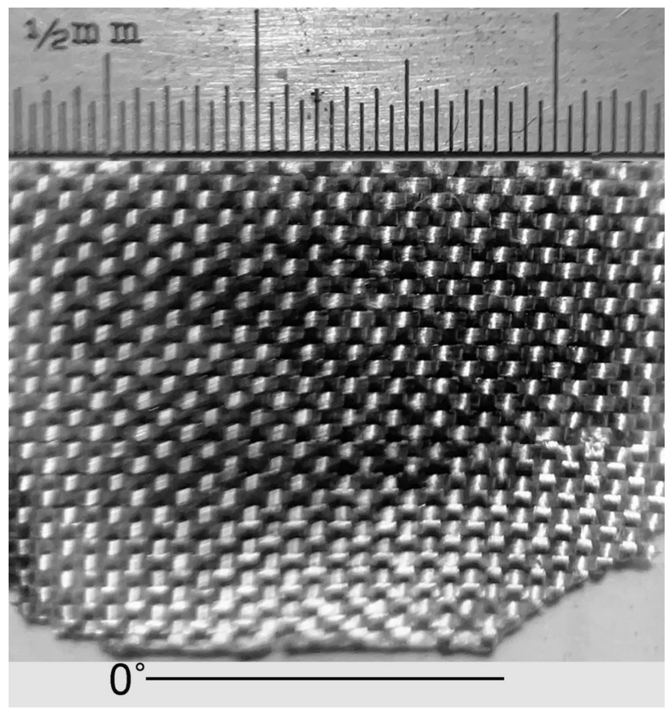
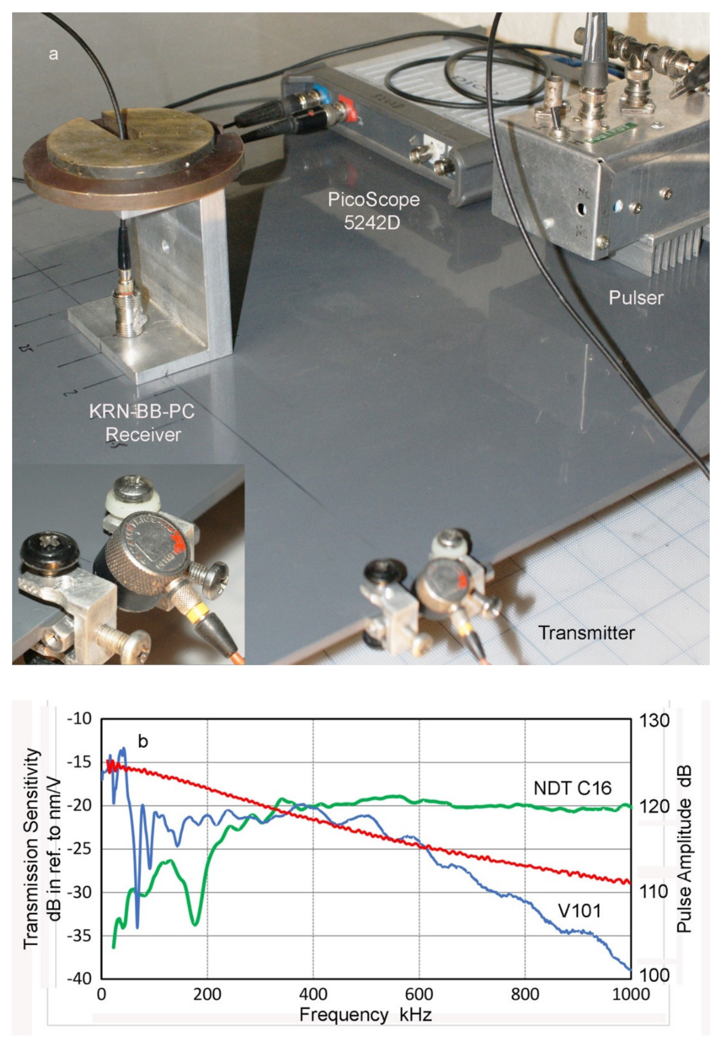
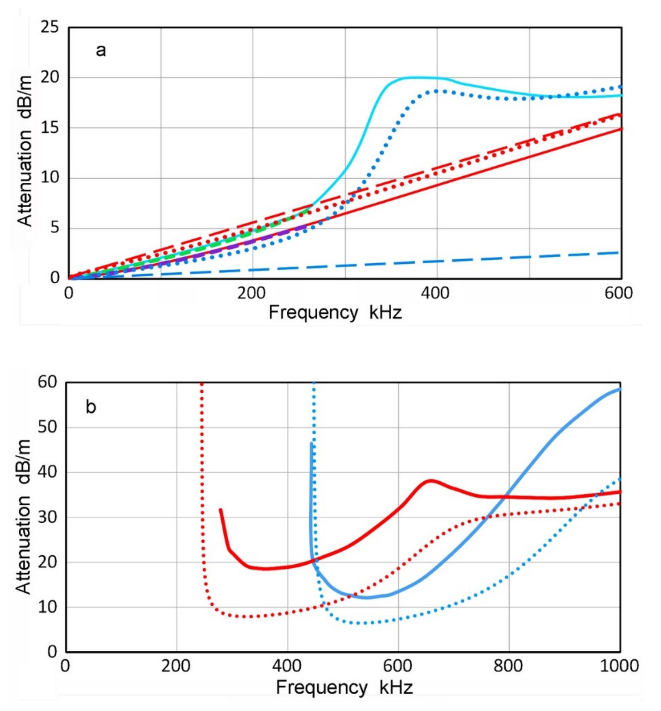
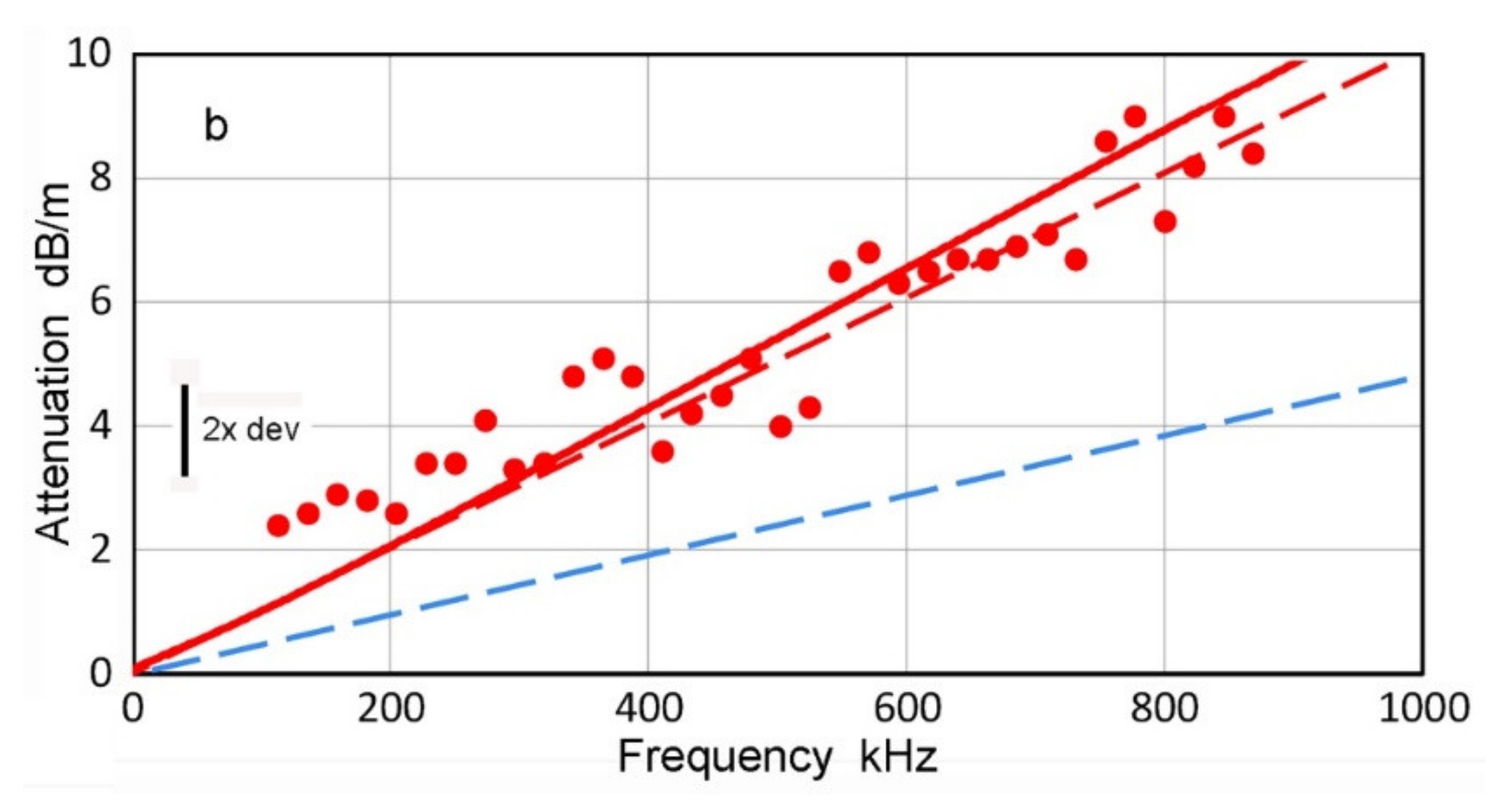
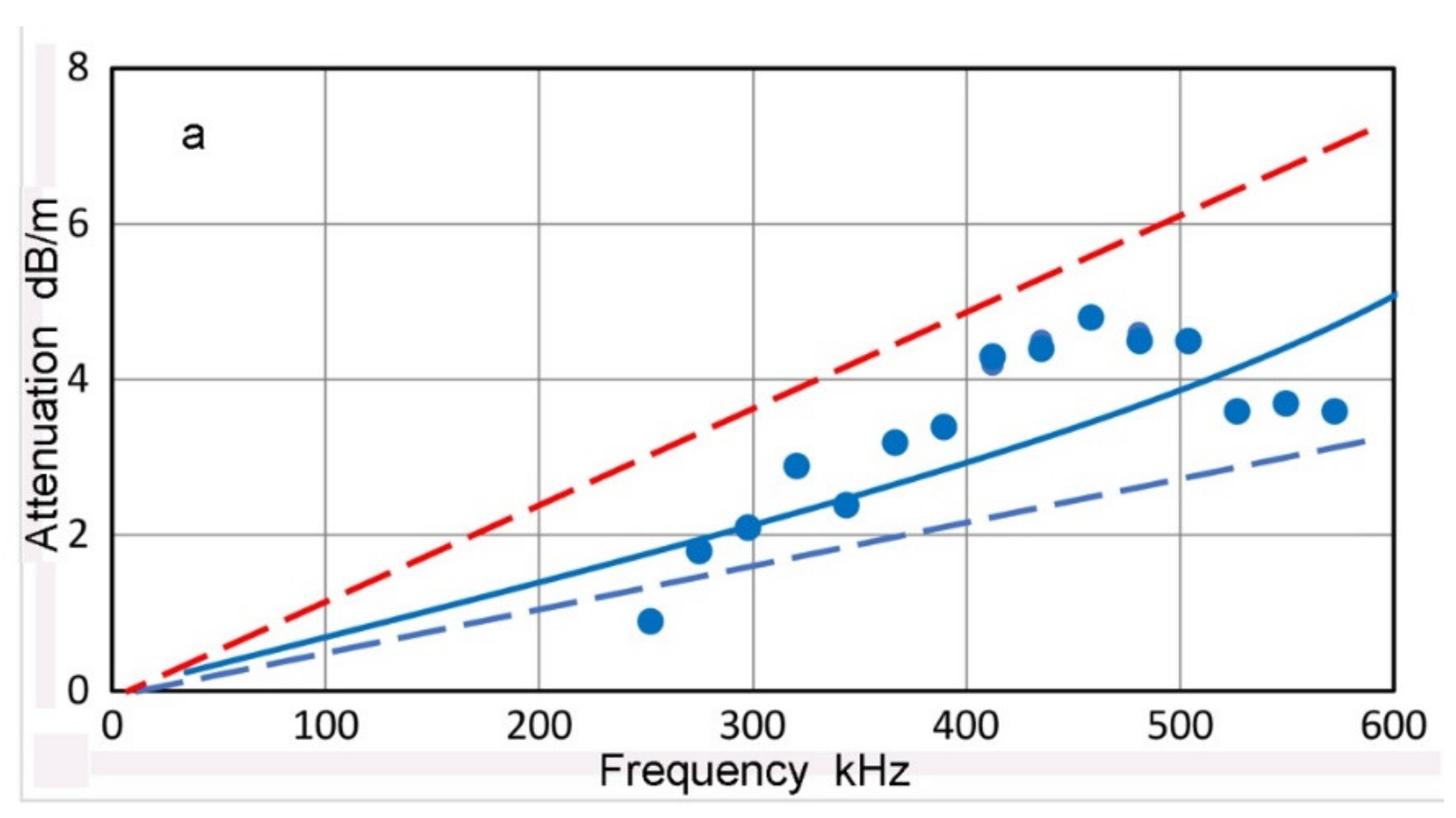
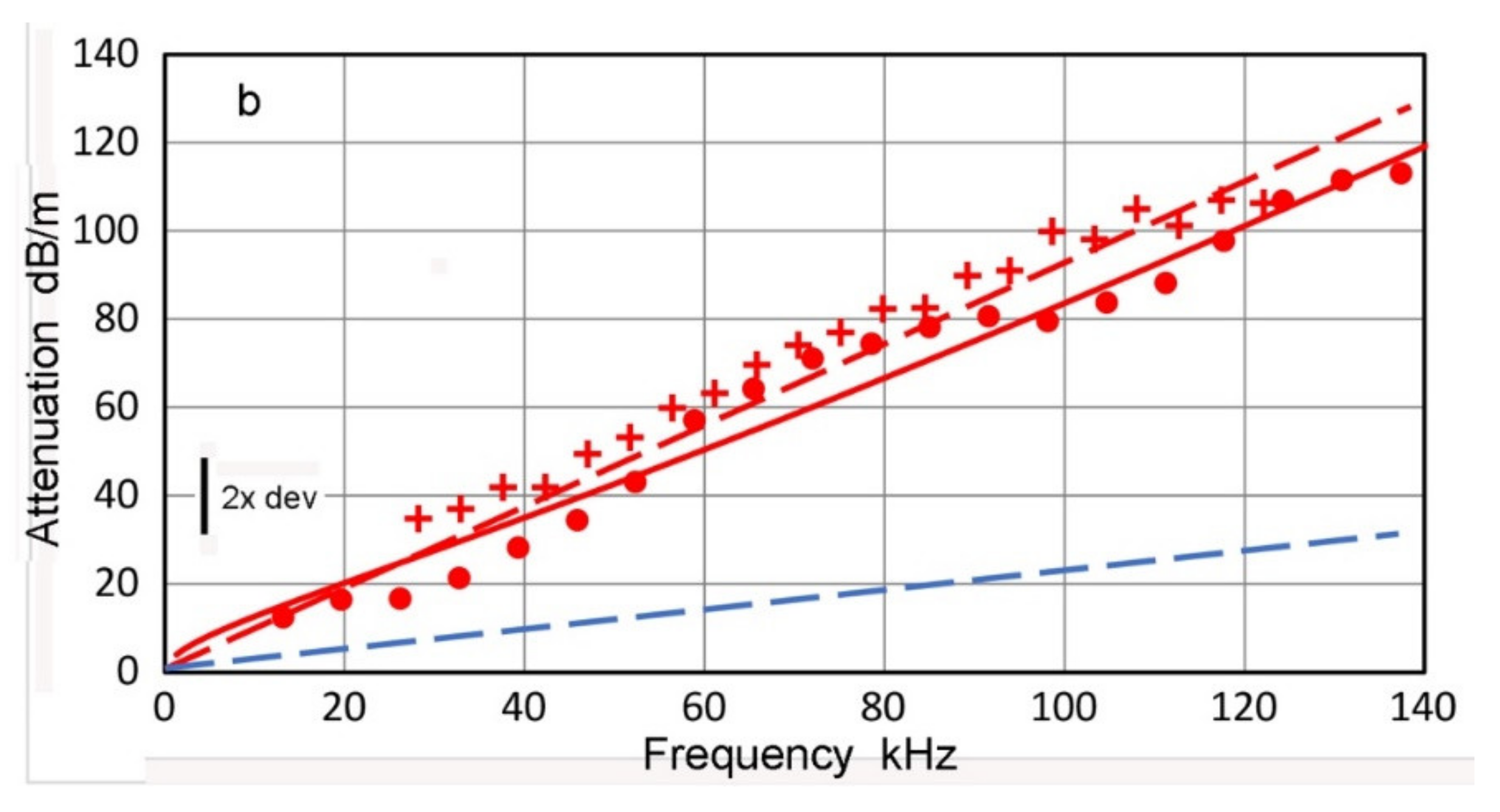
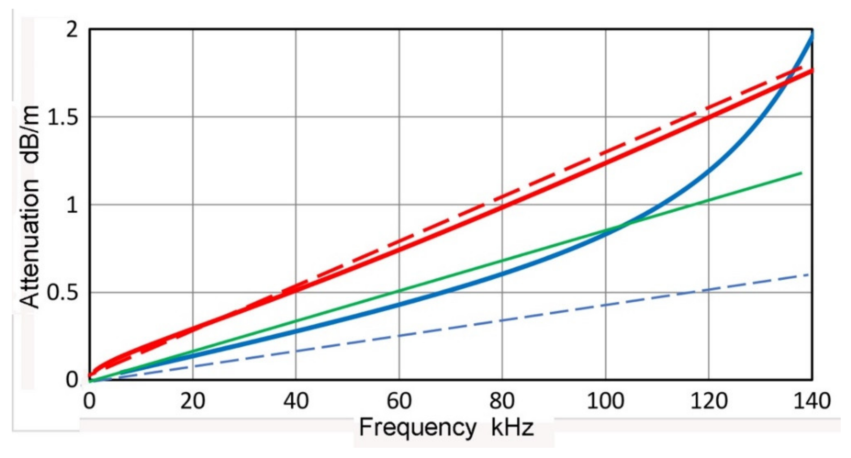
Table A1.
Calculation example.
| Lamb Wave Attenuation Using A-B Parameters | |||||||||
|---|---|---|---|---|---|---|---|---|---|
| One needs bulk wave attenuation coefficients, αL and αT, Rayleigh wave wavelength L (at 1 MHz), Rayleigh wave velocity VR and half-thickness d | |||||||||
| Units: αL and αT dB/m/MHz; L mm-MHz, VL mm/µs; d mm | |||||||||
| Example: 410 Stainless Steel, | |||||||||
| aL = 0.97 dB/m/MHz | aT = 2.6 dB/m/MHz | ||||||||
| L = 3.07 mm (1 MHz) | |||||||||
| VR = 3.07 mm/µs | |||||||||
| 2d = 5 mm | |||||||||
| Steel | VR=3.07 | 2d = 5 | Freq f in MHz | (αL) × f | (αT) × f | Freq in kHz | Attn from αL | Attn from αT | Total attn |
| From A–B Table 0.28 | (2d/L) VR/2d | 1000 × col D | dB/m | dB/m | dB/m | ||||
| 2d/L | A So | B So | col A × 3.07/5 | 0.97 × f | 2.6 × f | 2d = 5 mm | col B × col E | col C × col F | col H + col I |
| 0.0127 | 0.6231 | 0.2732 | 0.007826 | 0.007591 | 0.020347 | 7.8258 | 0.0047 | 0.0056 | 0.0103 |
| 0.0325 | 0.6150 | 0.2703 | 0.019940 | 0.019341 | 0.051843 | 19.9396 | 0.0119 | 0.0140 | 0.0259 |
| 0.0522 | 0.6170 | 0.2705 | 0.032050 | 0.031089 | 0.083331 | 32.0502 | 0.0192 | 0.0225 | 0.0417 |
| 0.0719 | 0.6144 | 0.2719 | 0.044155 | 0.042831 | 0.114804 | 44.1553 | 0.0263 | 0.0312 | 0.0575 |
| 0.0916 | 0.6147 | 0.2722 | 0.056253 | 0.054565 | 0.146257 | 56.2529 | 0.0335 | 0.0398 | 0.0734 |
| 0.1113 | 0.6117 | 0.2737 | 0.068341 | 0.066290 | 0.177686 | 68.3406 | 0.0406 | 0.0486 | 0.0892 |
A partial table gives how Lamb-wave attenuation coefficients are obtained. Cols. A to C (in yellow background) come from A–B table and represent 2d/L, A, and B (in this case for So). Col. D gives frequency, f, using Col. A, VR, and 2d (in MHz). Cols. E and F calculate bulk-wave attenuation. Col. G converts f into kHz unit (may be omitted). Cols. H and I calculate Lamb-wave attenuation due to αL and αT by multiplying A and B parameters. Col. J provides Lamb-wave attenuation coefficients (in dB/m) by summing Cols. H and I.
An Excel file, A-B parameters table, including two cases of Poisson’s ratio, 0.28 and 0.34, is available as Supplementary Material.
References
- Kishoni, D.; Workman, G.L.; Moore, P.O. (Eds.) Nondestructive Testing Handbook, 3rd ed.; Ultrasonic Testing; American Society for Nondestructive Testing: Columbus, OH, USA, 2007; Volume 7, 600p, ISBN 978-1-57117-105-4. [Google Scholar]
- Miller, R.K.; Hill, E.v.K.; Moore, P.O. (Eds.) Nondestructive Testing Handbook, 3rd ed.; Acoustic Emission Testing; American Society for Nondestructive Testing: Columbus, OH, USA, 2005; Volume 6, 446p, ISBN 978-1-57117-106-1. [Google Scholar]
- Boller, C.; Chang, F.K.; Fujino, Y. (Eds.) Encyclopedia of Structural Health Monitoring; Wiley: Hoboken, NJ, USA, 2009; 2960p. [Google Scholar]
- Quintanilla, F.H.; Fan, Z.; Lowe, M.; Craster, R.V. Guided waves’ dispersion curves in anisotropic viscoelastic single- and multi-layered media. Proc. R. Soc. A Math. Phys. Eng. Sci. 2015, 471, 20150268. [Google Scholar] [CrossRef]
- Croxford, A.J.; Wilcox, P.; Drinkwater, B.W.; Konstantinidis, G. Strategies for guided-wave structural health monitoring. Proc. R. Soc. A Math. Phys. Eng. Sci. 2007, 463, 2961–2981. [Google Scholar] [CrossRef]
- Sause, M.; Hamstad, M. Acoustic Emission Analysis. In Comprehensive Composite Materials II; Elsevier: Amsterdam, The Netherlands, 2018; Volume 7, pp. 291–326. [Google Scholar] [CrossRef]
- Meleshko, V.V.; Bondarenko, A.A.; Dovgiy, S.A.; Trofimchuk, A.N.; van Heijst, G.J.F. Elastic waveguides: History and the state of the art. I. J. Math. Sci. 2009, 162, 99–120. [Google Scholar] [CrossRef]
- Meleshko, V.V.; Bondarenko, A.A.; Trofimchuk, A.N.; Abasov, R.Z. Elastic waveguides: History and the state of the art. II. J. Math. Sci. 2010, 167, 197–216. [Google Scholar] [CrossRef]
- Green, A.T.; Lockman, C.S.; Steele, R.K. Acoustic verification of structural integrity of Polaris chambers. Mod. Plast. 1964, 41, 137–139. [Google Scholar]
- Fowler, T.J.; Blessing, J.A.; Conlisk, P.J.; Swanson, T.L. The MONPAC system. J. Acoust. Emiss. 1989, 8, 1–10. [Google Scholar]
- Hutton, P.H.; Jolly, W.D.; Vetrano, J.B. Acoustic emission for periodic and continuous flaw detection in pressure vessels. In US-Japan Joint Symp. on Acoustic Emission; High Pressure Inst.: Tokyo, Japan, 1972; pp. 53–172. [Google Scholar]
- Graham, L.J.; Alers, G.A. Acoustic emission in the frequency domain. In Monitoring Structural Integrity by Acoustic Emission; STP-571; American Society for Testing and Materials: Philadelphia, PA, USA, 1975; pp. 11–395. [Google Scholar]
- Pollock, A.A. Classical wave theory in practical AE testing. In Progress in AE III; The Japanese Society for Non-Destructive Inspection: Tokyo, Japan, 1986; pp. 708–721. [Google Scholar]
- Ono, K. Review on structural health evaluation with acoustic emission. Appl. Sci. 2018, 8, 958. [Google Scholar] [CrossRef] [Green Version]
- Gorman, M.R. Plate wave acoustic emission. J. Acoust. Soc. Am. 1991, 90, 358. [Google Scholar] [CrossRef]
- Hamstad, M.A.; Gary, J.; O’Gallagher, A. Far-field acoustic emission waves by three-dimensional finite element modeling of pencil-lead breaks on a thick plate. J. Acoust. Emiss. 1996, 14, 103–114. [Google Scholar]
- Suzuki, H.; Kinjo, T.; Hayashi, Y.; Takemoto, M.; Ono, K.; Hayashi, Y. Wavelet transform of acoustic emission signals. J. Acoust. Emiss. 1996, 14, 69–84. [Google Scholar]
- AGU-Vallen Wavelet Program; Vallen Systeme: Wolfratshausen, Germany, 2003.
- Viktorov, I.A. Rayleigh and Lamb Waves, Physical Theory and Applications; Plenum Press: New York, NY, USA, 1967; 154p. [Google Scholar]
- Krautkramer, J.; Krautkramer, H. Ultrasonic Testing of Materials; Springer: Berlin, Germany, 1969; 521p. [Google Scholar]
- The Japan Society for the Promotion of Science (Ed.) Ultrasonic Material Testing; Nikkan Kogyo: Tokyo, Japan, 1973; 818p. [Google Scholar]
- Cawley, P.; Alleyne, D. The use of Lamb waves for the long-range inspection of large structures. Ultrasonics 1996, 34, 287–290. [Google Scholar] [CrossRef]
- Lowe, M.; Alleyne, D.; Cawley, P. Defect detection in pipes using guided waves. Ultrasonics 1998, 36, 147–154. [Google Scholar] [CrossRef]
- Alleyne, D.N.; Pavlakovic, B.N.; Lowe, M.J.S.; Cawley, P. Rapid long-range inspection of chemical plant pipework using guided waves. Insight—Non-Destr. Test. Cond. Monit. 2001, 43, 93–96. [Google Scholar]
- Lowe, M.; Cawley, P.; Pavlakovic, B. Disperse: A general purpose computer model for calculating elastic waveguide properties, with application to non-destructive testing. In Surface Waves in Anisotropic and Laminated Bodies and Defects Detection; Goldstein, R.V., Maugin, G.A., Eds.; Kluwer: Amsterdam, The Netherlands, 2004; pp. 241–256. [Google Scholar]
- Lowe, M. Disperse|Research Groups|Imperial College London. Available online: http://www.imperial.ac.uk/non-destructiveevaluation/products-and-services/disperse/ (accessed on 27 January 2022).
- Huber, A. The Dispersion Calculator: A Free Software for Calculating Dispersion Curves of Guided Waves in Multilayered Composites. Available online: https://www.dlr.de/zlp/en/desktopdefault.aspx/tabid-14332/24874_read-61142/ (accessed on 27 January 2022).
- Nayfeh, A.H. Wave Propagation in Layered Anisotropic Media; Elsevier: Amsterdam, The Netherlands, 1995; 331p. [Google Scholar]
- Mal, A.K.; Bar-Cohen, Y.; Lih, S.-S. Wave attenuation in fiber reinforced composites. In Mechanics and Mechanisms of Material Damping; ASTM STP 1169; Kinra, V.K., Wolfenden, A., Eds.; American Society for Testing and Materials: Philadelphia, PA, USA, 1992; pp. 245–261. [Google Scholar]
- Hayashi, T.; Song, W.J.; Rose, J.L. Guided wave dispersion curves for a bar with an arbitrary cross-section, a rod and rail example. Ultrasonics 2003, 41, 175–183. [Google Scholar] [CrossRef]
- Neau, G.; Lowe, M.J.S.; Deschamps, M. Propagation of Lamb waves in anisotropic and absorbing plates: Theoretical derivation and experiments. In AIP Conference Proceedings; AIP Publishing: Melville, NY, USA, 2002; Volume 615, pp. 1062–1069. [Google Scholar] [CrossRef]
- Drinkwater, B.W.; Castaings, M.; Hosten, B. The measurement of and Lamb wave attenuation to determine the normal and shear stiffnesses of a compressively loaded interface. J. Acoust. Soc. Am. 2003, 113, 3161. [Google Scholar] [CrossRef]
- Bartoli, I.; Marzani, A.; Lanza di Scalea, F.; Viola, E. Modeling wave propagation in damped waveguides of arbitrary cross-section. J. Sound Vib. 2006, 295, 685–707. [Google Scholar] [CrossRef]
- Schmidt, D.; Sadri, H.; Szewieczek, A.; Sinapius, M.; Wierach, P.; Siegert, I.; Wendemuth, A. Characterization of Lamb wave attenuation mechanisms. In Health Monitoring of Structural and Biological Systems 2013; Proc. SPIE 8695; SPIE: San Diego, CA, USA, 2013; pp. 869503-1–869503-7. [Google Scholar] [CrossRef]
- Kamal, A.; Gresil, M.; Giurgiutiu, V. Comparative study of several methods for the calculation of ultrasonic guided waves in composites. In Proceedings of the 54th AIAA Structures, Structural Dynamics, and Materials Conference, Boston, MA, USA, 8–11 April 2013. [Google Scholar] [CrossRef] [Green Version]
- Gresil, M.; Giurgiutiu, V. Prediction of attenuated guided waves propagation in carbon fiber composites using Rayleigh damping model. J. Intell. Mater. Syst. Struct. 2014, 26, 2151–2169. [Google Scholar] [CrossRef]
- Deng, M. Analysis of second-harmonic generation of Lamb modes using a modal analysis approach. J. Appl. Phys. 2003, 94, 4152–4159. [Google Scholar] [CrossRef]
- Müller, M.F.; Kim, J.-Y.; Qu, J.; Jacobs, L.J. Characteristics of second harmonic generation of Lamb waves in nonlinear elastic plates. J. Acoust. Soc. Am. 2010, 127, 2141. [Google Scholar] [CrossRef] [Green Version]
- Matsuda, N.; Biwa, S. Frequency dependence of second-harmonic generation in Lamb waves. J. Nondestruct. Eval. 2014, 33, 169–177. [Google Scholar] [CrossRef] [Green Version]
- Mizutani, Y.; Yamada, H.; Nishino, H.; Takemoto, M.; Ono, K. Non-contact detection of delaminations in impacted cross-ply CFRP using laser generated Lamb waves. In Advanced Nondestructive Evaluation for Structural and Biological Health Monitoring; Proc. SPIE 4335; Kundu, T., Ed.; SPIE: San Diego, CA, USA, 2001; pp. 330–341. [Google Scholar] [CrossRef] [Green Version]
- Staszewski, W.J.; Lee, B.C.; Traynor, R. Fatigue crack detection in metallic structures with Lamb waves and 3D laser vibrometry. Meas. Sci. Technol. 2007, 18, 727–739. Available online: stacks.iop.org/SMS/13/251 (accessed on 10 June 2018). [CrossRef]
- Olisa, S.C.; Khan, M.A.; Starr, A. Review of current guided wave ultrasonic testing (GWUT) limitations and future directions. Sensors 2021, 21, 811. [Google Scholar] [CrossRef]
- Imperial College, London, UK. Available online: https://www.imperial.ac.uk/non-destructive-evaluation/publications/phd-theses/ (accessed on 10 April 2022).
- Ono, K. A comprehensive report on ultrasonic attenuation of engineering materials, including metals, ceramics, polymers, fiber-reinforced composites, wood, and rocks. Appl. Sci. 2020, 10, 2230. [Google Scholar] [CrossRef] [Green Version]
- Ono, K. Dynamic viscosity and transverse ultrasonic attenuation of engineering materials. Appl. Sci. 2020, 10, 5265. [Google Scholar] [CrossRef]
- Prosser, W.H. Ultrasonic Characterization of the Nonlinear Elastic Properties of Unidirectional Graphite/Epoxy Composites, NASA-CR-4100; Johns Hopkins University: Baltimore, MD, USA, 1987; 198p. [Google Scholar]
- Roman, I.; Ono, K. Acoustic emission characterization of failure mechanisms in Woven roving glass-epoxy composites. In Progress in Acoustic Emission II; Japanese Society for Non-Destructive Inspection: Tokyo, Japan, 1984; pp. 496–503. [Google Scholar]
- Ono, K.; Gallego, A. Attenuation of Lamb waves in CFRP plates. J. Acoust. Emiss. 2012, 30, 109–123. [Google Scholar]
- Ono, K.; Cho, H.; Vallen, H.; M’Closkey, R.T. Transmission sensitivities of contact ultrasonic transducers and their applications. Sensors 2021, 21, 4396. [Google Scholar] [CrossRef]
- Ono, K. Rayleigh wave calibration of acoustic emission sensors and ultrasonic transducers. Sensors 2019, 19, 3129. [Google Scholar] [CrossRef] [Green Version]
- Lowe, M.; Pavlakovic, B. Disperse: A System for Generating Dispersion Curves; Users’ Manual, ver. 2.0.20a; Imperial College: London, UK, 2013; 207p. [Google Scholar]
- Staszewski, W.J.; Lee, B.C.; Mallet, L.; Scarpa, F. Structural health monitoring using scanning laser vibrometry: I. Lamb wave sensing. Smart Mater. Struct. 2004, 13, 251–260. [Google Scholar] [CrossRef]
Figure 1.
Woven rovings of glass fiber cloth after burning the matrix resin. Lamb wave propagation was along 0° direction marked. Top scale has 0.5 mm spacing.
Figure 1.
Woven rovings of glass fiber cloth after burning the matrix resin. Lamb wave propagation was along 0° direction marked. Top scale has 0.5 mm spacing.

Figure 2.
(a) Experimental set-up for attenuation measurement of asymmetric mode with a plate sample. A transducer glued to a hex rod is coupled to a plate edge using a pair of jigs. See also enlarged insert. Receiving sensor, a pulser and an oscilloscope are also visible. (b) Transmission sensitivity of two transducers, Olympus V101 (blue curve) and NDT C16. (green curve) in dB in reference to 1 nm/V. Normal incidence. Frequency spectrum of an excitation pulse is given in red. (c) Displacement output spectra of Olympus V103 (in blue) and NDT C16 (in red). Transducer mounted on a hex rod: 60° incidence. The dB scale is relative due to partial coupling to a calibrated receiver. (d) Rayleigh wave receiving sensitivity of two sensors, KRN-BB-PC (in green) and PAC Pico (in red). The dB scale is in reference to 1 mV/pm.


Figure 3.
(a) Displacement amplitude (in pm) of symmetric Lamb waves detected on front side (blue curve), back side (green curve) and summed (halved, red curve) on 1.4-mm PS sheet. Propagation distance: 200 mm. Signal arrival: 97 µs, Transmitter (Tx): NDT C16 (normal incidence), Receiver (Rx): KRN-BB-PC. (b) Displacement amplitude (in pm) of asymmetric Lamb waves. Same sample and transducers as above except halved signal difference is shown as red curve, Tx incident angle of 60° used and signal arrival at 169 µs (plotted from 170 µs). (c) Wavelet transform spectrogram of the summed signal (red curve, (a)). Transform start time was shifted by 97 µs. Red and blue represent high and low WT intensities. Dispersion curves for So and Ao modes are also plotted. Insert shows a partial WT spectrogram at propagation distance of 125 mm, shifted by 60 µs. (d) Wavelet transform spectrogram of the difference signal (red curve, (b)). Transform start time was shifted by 169 µs. Dispersion curves for So, Ao and A1 modes plotted. (e) WT intensity sum, D√x, in dB vs. propagation distance, x, for symmetric Lamb waves on 1.4-mm PS sheet. The slope from the linear regression fit gives So-mode attenuation coefficient, α–So at 496 kHz. (f) α–So values vs. frequency. One of them came from (e), Blue dotted curve shows a fourth order polynomial fit to α-So data.


Figure 4.
(a) Theoretical calculations of Lamb wave attenuation from Viktorov [19] and Disperse program [25,51] for an isotropic Al plate (6.4-mm thickness) with Poisson’s ratio of 0.34. α–So: Solid blue curve for Viktorov with its transverse attenuation component shown by dashed green curve. Dotted blue curve for Disperse. α–Ao: Solid red curve for Viktorov with its transverse attenuation component shown by dashed purple curve. Dotted red curve for Disperse. αL and αT: Blue and red long-dash lines. (b) Same as in (a). α–S1: Solid blue curve for Viktorov. Dotted blue curve for Disperse. α–A1: Solid red curve for Viktorov. Dotted red curve for Disperse. (c). Theoretical calculations of Lamb wave attenuation using Disperse [25,51] for an isotropic Al-1100 plate (6.4-mm thickness, but higher αL and αT). Solid blue curve for α–So with its transverse attenuation component shown by dotted blue curve. Blue dash-dotted curve is percent contribution of transverse attenuation component to α–So, obtained by the parametric method (right scale). αL and αT: Blue and red dash lines. (d) Theoretical calculations of Lamb wave attenuation using Disperse [25,51] for an isotropic Al-1100 plate (6.4-mm thickness, but higher αL and αT). Solid red curve for α–Ao with its transverse attenuation component shown by dotted red curve. Red dash-dotted curve is percent contribution of transverse attenuation component to α–Ao, obtained by the parametric method (right scale). αL and αT: Blue and red dash lines.


Figure 5.
(a) α–So for PS sheets of 1.4-mm thickness in blue symbols. α–S values plotted in dots used Olympus V101 as Tx and + symbols NDT C16 as Tx. KRN-BB-PC was Rx for both. Calculated values of α–So are plotted in a solid blue curve. Blue and red dashed lines are the bulk-wave attenuation coefficients, αL and αT. Vertical bar indicates twice the value of average deviation or 2 × dev. (b) α–Ao for PS sheets of 1.4-mm thickness in red symbols. Tx for all three sets used NDT C16 at 60° incident angle. KRN-BB-PC was Rx for all three. Calculated values of α–Ao are plotted in a solid red curve. Blue and red dashed lines are the bulk-wave attenuation coefficients, αL and αT. Vertical bar shows 2 × dev.

Figure 6.
(a) α–So values for Al-1100 sheet of 2.1-mm thickness in blue symbols. α–So values plotted in dots used PAC Pico as Tx and + symbols KRN-BB-PCP as Tx. Both Tx’s were attached on the end face. KRN-BB-PC was Rx for both. Calculated values of α–So are plotted in a solid blue curve. αL and αT: Blue and red dash lines. Vertical bar shows 2 × dev. (b) Four sets of α–Ao values for Al-1100 sheet of 2.1-mm thickness are plotted in red symbols. Data with + symbols used NDT C16 Tx at 60° incident angle, dot, diamond and triangle symbols used surface-mounted KRN-BB-PCP Tx, located near edge, which allowed firm clamping and two-surface detection approach. The dot data used 200-kHz sinewave pulse, while the rest used short-pulse excitation. KRN-BB-PC was Rx for all four. Calculated α–Ao (solid red curve), αL and αT (blue and red dashed lines) are plotted as in Figure 5b. Vertical bar shows 2 × dev.

Figure 7.
(a) α–So values for Al 1100 plate of 6.4-mm thickness plotted in blue squares used Olympus V101 as Tx and KRN-BB-PC as Rx. Calculated α–So (solid blue curve), αL and αT (blue and red dashed lines) are also plotted. Vertical bar shows 2 × dev. (b) α–Ao values for Al 1100 sheet of 6.4-mm thickness plotted in red dot symbols, using short-pulse excited NDT C16 Tx at 60° incident angle and KRN-BB-PC Rx. Calculated α–Ao (solid red curve), αL and αT (blue and red dashed lines) are also plotted. Vertical bar shows 2 × dev.

Figure 8.
(a) α–So values for Al-6061 plate of 12.7-mm thickness. Blue + symbols are for the data with 100-kHz excitation, while blue dots used 200-kHz excitation. Tx: AET FC500, Rx: KRN-BB-PC. Calculated α–So (solid blue curve), αL and αT (blue and red dashed lines) are also plotted. Vertical bar shows 2 × dev. (b) α–Ao values for Al-6061 plate of 12.7-mm thickness. Red dots are for the data using short-pulse excited AET FC500 as Tx and KRN-BB-PC as Rx. Calculated α–Ao (solid red curve), αL and αT (blue and red dashed lines) are also plotted. Vertical bar shows 2 × dev.


Figure 9.
(a) Received signal and its WT spectrogram of α–So test for Al-6061 plate of 12.7-mm thickness with 100-kHz excitation at 400 mm from the source. Transform start time was shifted by 75 µs. Red and blue represent high and low WT intensities. Dispersion curves for So, Ao and A1 modes are also plotted. (b) Received signal and its WT spectrogram of α–So test for Al-6061 plate of 12.7-mm thickness with 200-kHz excitation at 400 mm from the source. Transform start time was shifted by 185 µs. Red and blue represent high and low WT intensities. Dispersion curves for So and A1 modes are also plotted.


Figure 10.
(a) α–So values for Al-7475 of 2.7-mm thickness. Blue dots are for the data with Olympus V101 as Tx and KRN-BB-PC as Rx. Calculated α–So (solid blue curve), αL and αT (blue and red dashed lines) are also plotted. (b) α–Ao values for Al-7475 of 2.7-mm thickness. Red + symbols for short-pulse excited KRN-BB-PCP as Tx and KRN-BB-PC as Rx. Calculated α–Ao (solid red curve), αL and αT (blue and red dashed lines) are also plotted. Additionally, red dotted and dash-dotted lines are drawn to represent 2 αT and 3 αT lines.


Figure 11.
(a) α–So values for 410SS sheet of 3.2-mm thickness plotted in blue dots with Olympus V101 as Tx and KRN-BB-PC as Rx. Calculated α–So (solid blue curve), α–S1 (blue dotted), αL and αT (blue and red dashed lines) are also plotted. (b) α–Ao values for 410SS sheet of 3.2-mm thickness plotted in red dot symbols, using short-pulse excited NDT C16 Tx at 60° incident angle and KRN-BB-PC Rx. Calculated α–Ao (solid red curve), α–A1 (red dotted), αL and αT (blue and red dashed lines) are also plotted.

Figure 12.
(a) Three sets of α–So values for soda lime glass sheet of 2.0-mm thickness. All with Olympus V103 as Tx and KRN-BB-PC as Rx. Blue dots: Single-cycle sinewave at 600 kHz, Blue squares: Single-cycle sinewave at 750 kHz, Blue triangles: Single-cycle sinewave at 750 kHz, one-surface detection. Calculated α–So (solid blue curve), αL and αT (blue and red dashed lines) are also plotted. Blue dotted curve was also for α–So, but calculated using reduced αL and αT (see text). Vertical bar shows 2 × dev. (b) Two sets of α–Ao values for soda lime glass sheet of 2.0-mm thickness plotted in red symbols. Both sets used single-cycle sinewave at 600 kHz with Olympus V103 Tx at 60° incident angle and KRN-BB-PC Rx. Calculated α–Ao (solid red curve), αL and αT (blue and red dashed lines) are also plotted. α–Ao (red dotted) used reduced αL and αT (see text). Vertical bar shows 2 × dev.

Figure 13.
(a) α–S values for soda lime glass sheet of 4.7-mm thickness. All with Olympus V101 as Tx and KRN-BB-PC as Rx. Calculated α–So (solid blue curve), α–S1 (dotted blue curve), αL and αT (blue and red dashed lines) are also plotted. Vertical bar shows 2 × dev of data below 600 kHz. (b) Two sets of α–Ao values for soda lime glass sheet of 4.7-mm thickness plotted in red symbols. Both sets used short-pulse excited NDT C16 Tx at 60° incident angle and KRN-BB-PC Rx. Calculated α–Ao (solid red curve), α–A1 (dotted red curve), αL and αT (blue and red dashed lines) are also plotted. Vertical bar shows 2 × dev.

Figure 14.
(a) Observed α–So values for 1.8-mm PMMA sheet along with the calculated attenuation and dashed lines for αL and αT. Three test series are plotted using blue symbols. Dot data used Olympus V101 Tx and PAC Pico Rx, + symbols used Olympus V101 Tx and KRN-BB-PC Rx and triangles used NDT C16 Tx and KRN-BB-PC Rx. All with short-pulse excitation. Vertical bar shows 2 × dev. (b) Observed α–Ao values for 1.8-mm PMMA sheet along with the calculated attenuation and dashed lines for αL and αT. Three test series are plotted using red symbols. Dots used KRN-BB-PCP Tx on the sheet 5 mm from an edge and KRN-BB-PC Rx, + symbols used NDT C16 Tx at 60° incident angle and PAC Pico Rx, and triangles also used NDT C16, but with KRN-BB-PC Rx. All with short-pulse excitation. Vertical bar shows 2 × dev.

Figure 15.
(a) Observed α–So values for 6.3-mm PMMA plate along with the calculated attenuation and dashed lines for αL and αT. Three test series are plotted using blue symbols. Dot and triangle data used Olympus V101 Tx and PAC Pico Rx, and + symbols used Olympus V101 Tx and KRN-BB-PC Rx. All with short-pulse excitation. Vertical bar shows 2 × dev. (b) Observed α–Ao values for 6.3-mm PMMA plate along with the calculated attenuation and dashed lines for αL and αT. Three test series are plotted using red symbols. Dot and triangle data used Olympus V103 Tx and NDT C16 Tx at 60° incident angle, respectively, with PAC Pico Rx, and + symbols used Olympus V221 Tx and KRN-BB-PC Rx. The poling direction of V221 was oriented to match the plate surface normal. All with short-pulse excitation. Vertical bar shows 2 × dev.

Figure 16.
(a) Observed α–So values for 4.3-mm PVC plate along with the calculated attenuation and dashed lines for αL and αT. Two test series are plotted using blue symbols. Both used Olympus V101 Tx and KRN-BB-PC Rx, with short-pulse excitation. Vertical bar shows 2 × dev. (b) Observed α–Ao values for 4.3-mm PVC plate along with the calculated attenuation and dashed lines for αL and αT. Both series are plotted using red symbols and used NDT C16 Tx at 60° incident angle and KRN-BB-PC Rx. All with short-pulse excitation. Vertical bar shows 2 × dev.


Figure 17.
(a) Observed α–So values for 7.1-mm HDPE plate with the calculated attenuation and dashed lines for αL and αT. Two test series are plotted using blue symbols. Both used Olympus V101 Tx and KRN-BB-PC Rx, with short-pulse excitation. Vertical bar shows 2 × dev. (b) Observed α–S values for 7.1-mm HDPE plate along with the calculated attenuation and dashed lines for αL and αT. Frequency range was extended to 500 kHz. Two test series and their symbols are identical to those in (a). Calculated attenuation curves included α–S1 (blue dotted curve) and α–S2 (blue short-dash curve). (c) Observed α–Ao values for 7.1-mm HDPE plate using red symbols. Dot data used NDT C16 Tx at 60° incident angle with 50-kHz single-cycle sinewave excitation and KRN-BB-PC Rx. The other two series used NDT C16 Tx at 60° incident angle with short-pulse excitation and KRN-BB-PC Rx. The calculated attenuation and dashed lines for αL and αT are also plotted. Vertical bar shows 2 × dev.

Figure 18.
(a) Observed α–So values for 2.3-mm XP-GFRP sheet with the calculated attenuation and dashed lines for αL (=α33) and αT (=α32). Blue dotted line is for αL = α22, showing differences in 0° and 90° directions. Two test series are plotted using blue symbols. Both used Olympus V101 Tx and KRN-BB-PC Rx. Data with + symbols used short-pulse excitation and dot data used 400-kHz Gaussian pulse. (b) Observed α–Ao values for 2.3-mm XP-GFRP sheet with the calculated attenuation and dashed lines for αL and αT (=α32). Red dotted line for αT = α32 is also plotted. Three data series are shown. Red dot data used Olympus V103 Tx and KRN-BB-PC Rx, red square data with AET AC375L Tx and PAC Pico Rx, and red + data with NDT C16 Tx and KRN-BB-PC Rx. All Tx used 60° incident angle and short-pulse excitation.


Figure 19.
Approximate estimation of α–So (green curve) and α–Ao (red dash line) values using αL and αT. Calculated α–So (blue curve) and α–Ao (red curve) for SM50 steel are also plotted.
Figure 19.
Approximate estimation of α–So (green curve) and α–Ao (red dash line) values using αL and αT. Calculated α–So (blue curve) and α–Ao (red curve) for SM50 steel are also plotted.

Figure 20.
A cross-plot of longitudinal and transverse attenuation coefficients, αL and αT, of 159 various solids. Solid blue line: αT = 2.79 αL, dotted blue line: αT = αL. Data are from [14,45].

Table 1.
Tested materials and their properties.
| Test | Material | Density | VL | VT | αL | αT | Thickness | Size | Hardness | Notes * |
|---|---|---|---|---|---|---|---|---|---|---|
| No. | Mg/m3 | mm/µs | dB/m/MHz | mm | mm × mm | VHN | ||||
| G1a | PS | 1.06 | 2.34 | 1.16 | 39 | 113 | 1.38 | 554 × 433 | αL and αT measured. * | |
| G1b | PS | 1.05 | 2.3 | 1.17 | 39 | 113 | 1.38 | 602 × 397 | αL and αT of G1a used. | |
| G2a | Al-1100-H18 | 2.7 | 6.18 | 3.08 | 15.7 | 26.5 | 2.06 | 1133 × 523 | 41 | αL and αT of G2b used. |
| G2b | Al-1100-H18 | 2.7 | 6.18 | 3.08 | 15.7 | 26.5 | 6.38 | 907 × 306 | 40 | αL and αT measured. |
| G3a | Al-6061-T6 | 2.7 | 6.38 | 3.23 | 4.9 | 10.3 | 12.7 | 1220 × 1200 | 109 | αL and αT of G3b used. |
| G3b | Al-6061-T6 | 2.7 | 6.4 | 3.17 | 4.9 | 10.3 | 25.3 | 63.5 × 47.3 | 122 | Only for damping tests. |
| G4 | Al-7475-H18 | 2.81 | 6.5 | 2.99 | 5.7 | 12.2 | 2.72 | 610 × 367 | 123 | αL and αT of N19 used. + |
| G5a | Stainless steel 410 | 7.74 | 5.74 | 3.11 | 0.97 | 2.6 | 3.16 | 1015 × 306 | 240 | αL and αT of G5b used. |
| G5b | Stainless steel 410 | 7.7 | 5.97 | 3.32 | 0.97 | 2.6 | 104.9 | (38.5 dia.) | 211 | Only for damping tests. |
| G6a | Soda-lime glass | 2.55 | 5.73 | 3.43 | 8.7 | 16.2 | 1.98 | 609 × 578 | αL and αT of C43 used. + | |
| G6b | Soda-lime glass | 2.49 | 5.9 | 3.3 | 8.7 | 16.2 | 4.72 | 820 × 450 | αL and αT of C43 used. + | |
| G7a | PMMA # | 1.18 | 2.74 | 1.4 | 131 | 420 | 1.76 | 430 × 338 | αL and αT measured. + | |
| G7b | PMMA # | 1.18 | 2.74 | 1.4 | 106 | 216 | 6.3 | 610 × 610 | αL and αT measured. | |
| G8 | PVC | 1.4 | 2.33 | 1.11 | 239 | 909 | 4.3 | 812 × 812 | αL and αT of O2c used. + | |
| G9 | HDPE | 0.95 | 2.18 | 1.13 | 222 | 1010 | 7.09 | 585 × 509 | αL and αT of O10 used. + | |
| G10 | XP-GFRP § | 1.81 | 3.84 | 1.99 | 117 | 445 | 2.3 | 555 × 277 | αL and αT measured. * | |
* Four sheets were glued for attenuation tests. + Test Numbers used in Notes for G4, G6a,b, G8 and G9 refer to those from [44,45]. # Values of VL and density of PMMA were incorrectly listed previously in [44,45]. § Isotropy assumed for V and α values listed above. Complete V and α values are listed below.
Table 2.
Summary of Lamb wave attenuation values at approximate center frequencies.
| Test | Material | αL | αT | Thickness | Symmetric | Asymmetric | Notes | ||||
|---|---|---|---|---|---|---|---|---|---|---|---|
| No. | dB/m/MHz | mm | Freq. kHz | α–So (dB/m) | Freq. kHz | α–Ao (dB/m) | |||||
| Theory | Exp. | Theory | Exp. | ||||||||
| G1 | PS | 39 | 113 | 1.38 | 300 | 19.7 | 16.4 | 350 | 37.4 | 34.3 | Average of two. |
| G2a | Al-1100-H18 | 15.7 | 26.5 | 2.06 | 350 | 5.77 | 5.6 | 250 | 7.44 | 7 | |
| G2b | Al-1100-H18 | 15.7 | 26.5 | 6.38 | 300 | 6.71 | 7.9 | 250 | 6.71 | 6.6 | |
| G3 | Al-6061-T6 | 2.7 | 6.38 | 12.7 | 150 | 1.27 | 1.9 | 450 | 4.84 | 4.3 | |
| G6a | Soda-lime glass | 8.7 | 16.2 | 1.98 | 525 | 5.15 | 3.7 | 450 | 7.42 | 6.8 | |
| G6b | Soda-lime glass | 8.7 | 16.2 | 4.72 | 300 | 3.15 | 1.5 | 500 | 8.12 | 7.8 | |
| G7a | PMMA | 131 | 420 | 1.76 | 200 | 44.6 | 47.8 | 250 | 98.2 | 117 | |
| G7b | PMMA | 106 | 216 | 6.3 | 200 | 67.5 | 68.7 | 250 | 55.5 | 56.6 | |
| G8 | PVC | 239 | 909 | 4.3 | 70 | 33.5 | 43.9 | 70 | 58.5 | 71.7 | |
| G9 | HDPE | 222 | 1010 | 7.09 | 60 | 33.1 | 43.8 | 60 | 55.1 | 54.1 | |
| G10 | XP-GFRP | 117 | 445 | 2.3 | 300 | 35.3 * | 43.6 | 80 | 36.7 | 40.5 | * αL value used. |
Table 3.
Peak displacement of detected Lamb-wave signals using a point contact sensor (KRN-BB-PC).
| Test | Material | Thickness | Symmetric | Asymmetric | ||
|---|---|---|---|---|---|---|
| No. | mm | Transmitter | Peak Amplitude | Transmitter | Peak Amplitude | |
| nm | nm | |||||
| G1 | PS | 1.38 | NDT C16 | 0.08 | NDT C16 | 0.117 |
| G2a | Al-1100-H18 | 2.06 | PAC Pico | 1.31 | NDT C16 | 0.39 |
| G2b | Al-1100-H18 | 6.38 | Oly. V101 | 1.46 | NDT C16 | 1 |
| G3 | Al-6061-T6 | 12.7 | PAC Pico | 0.125 | PAC Pico | 0.114 |
| G4 | Al-7475 | 2.72 | Oly. V101 | 0.62 | KRN-BB-PCP | 0.63 |
| G5 | 410SS | 3.16 | Oly. V101 | 0.36 | NDT C16 | 0.51 |
| G6a | Soda-lime glass | 1.98 | Oly. V103 | 1.31 | NDT C16 | 0.073 |
| G6b | Soda-lime glass | 4.72 | Oly. V101 | 0.43 | NDT C16 | 1.24 |
| G7a | PMMA | 1.76 | Oly. V101 | 0.01 | NDT C16 | 0.037 |
| G7b | PMMA | 6.3 | Oly. V101 | 0.047 | Oly. V103 | 0.034 |
| G8 | PVC | 4.3 | NDT C16 | 0.018 | NDT C16 | 0.014 |
| G9 | HDPE | 7.09 | Oly. V101 | 0.015 | NDT C16 | 0.017 |
| G10 | XP-GFRP | 2.3 | Oly. V101 | 0.26 | Oly. V103 | 0.036 |
Publisher’s Note: MDPI stays neutral with regard to jurisdictional claims in published maps and institutional affiliations. |
© 2022 by the author. Licensee MDPI, Basel, Switzerland. This article is an open access article distributed under the terms and conditions of the Creative Commons Attribution (CC BY) license (https://creativecommons.org/licenses/by/4.0/).
Share and Cite
MDPI and ACS Style
Ono, K. Experimental Determination of Lamb-Wave Attenuation Coefficients. Appl. Sci. 2022, 12, 6735. https://doi.org/10.3390/app12136735
AMA Style
Ono K. Experimental Determination of Lamb-Wave Attenuation Coefficients. Applied Sciences. 2022; 12(13):6735. https://doi.org/10.3390/app12136735
Chicago/Turabian StyleOno, Kanji. 2022. "Experimental Determination of Lamb-Wave Attenuation Coefficients" Applied Sciences 12, no. 13: 6735. https://doi.org/10.3390/app12136735
Note that from the first issue of 2016, this journal uses article numbers instead of page numbers. See further details here.