
Monitoring of Atmospheric Corrosion of Aircraft Aluminum Alloy AA2024 by Acoustic Emission Measurements

Institute of Structural Lightweight Design, Johannes Kepler University Linz, Altenberger Str. 69, 4040 Linz, Austria
*
Author to whom correspondence should be addressed.
Appl. Sci. 2023, 13(1), 370; https://doi.org/10.3390/app13010370
Submission received: 16 November 2022
/
Revised: 20 December 2022
/
Accepted: 21 December 2022
/
Published: 27 December 2022
(This article belongs to the Special Issue Elastic Waves and Acoustic Emission for Innovative Monitoring of Structures and Engineering Systems)
Abstract
:Atmospheric corrosion of aluminum aircraft structures occurs due to a variety of reasons. A typical phenomenon leading to corrosion during aircraft operation is the deliquescence of salt contaminants due to changes in the ambient relative humidity (RH). Currently, the corrosion of aircraft is controlled through scheduled inspections. In contrast, the present contribution aims to continuously monitor atmospheric corrosion using the acoustic emission (AE) method, which could lead to a structural health monitoring application for aircraft. The AE method is frequently used for corrosion detection under immersion-like conditions or for corrosion where stress-induced cracking is involved. However, the applicability of the AE method to the detection of atmospheric corrosion in unloaded aluminum structures has not yet been demonstrated. To address this issue, the present investigation uses small droplets of a sodium chloride solution to induce atmospheric corrosion of uncladded aluminum alloy AA2024-T351. The operating conditions of an aircraft are simulated by controlled variations in the RH. The AE signals are measured while the corrosion site is visually observed through video recordings. A clear correlation between the formation and growth of pits, the AE and hydrogen bubble activity, and the RH is found. Thus, the findings demonstrate the applicability of the AE method to the monitoring of the atmospheric corrosion of aluminum aircraft structures using current measurement equipment. Numerous potential effects that can affect the measurable AE signals are discussed. Among these, bubble activity is considered to cause the most emissions.
1. Introduction
The corrosion of aluminum is an issue that needs to be kept under control in the aircraft industry to ensure the safety and functionality of mechanical structures during operation. Due to its lightweight properties, aluminum is widely used for the structural components of aircraft. These can be exposed to various corrosive environments during operation. Common sources of corrosion-promoting environments in the aircraft industry are aqueous electrolytes, such as sea spray in coastal regions or at flight over the ocean at low altitudes, and system leaks of fluids, e.g., hydraulic oils, coolant fluids, or spillages inside the cabin such as soup, coffee, or mineral water [1,2,3,4]. Furthermore, moisture from rain, fog, or snow can combine with different pollutants, such as dirt, exhaust gases, sulfates, chlorides, etc., or electrically conductive and chemically reactive solutions that can corrode aluminum [2]. If soluble salt contaminants are present and the relative humidity (RH) is above the deliquescence relative humidity (DRH) of the particular salt contamination, the salt takes up water from the ambient atmosphere and forms a highly concentrated electrolyte [5]. Aircraft operate in different climate zones and altitudes, hence they are exposed to fast changes in temperature and RH, which can lead to condensation and, in combination with salts or other contaminants, to a corrosive solution [1,2,3,6]. Aside from leakages and spillages of larger amounts of electrolytes, the above-mentioned examples are typical sources of so-called atmospheric corrosion, which is the corrosion of a metal where the electrolyte is present in the form of a thin film, small droplets, or both [1,5,6].
Typically, the corrosion of the structural components of aircraft is kept under control through scheduled inspections and clear protocols on how to determine corrosion [3,7], whereas the aim of the present research is to develop a structural health monitoring (SHM) application for the future detection and monitoring of aircraft corrosion damage. Several research works can be found where corrosion issues of different industries are addressed using the non-destructive testing (NDT) and SHM methods. For example, electrochemical techniques, such as the electrochemical noise technique, show good potential for monitoring corrosion [8,9]. There are also methods based on electrochemical impedance spectroscopy that were tested in field applications several years ago [10]. Another group of monitoring methods is optical fiber-based techniques [11]. Several studies can be found on the monitoring of the corrosion of reinforced concrete in civil engineering [12], but fiber-optic techniques have also been tested for aircraft [13,14]. Besides the already mentioned methods, acoustic methods are also of great importance to the monitoring of corrosion. The most popular technique in this context is perhaps ultrasonic testing (UT) [15]. UT is well developed for ground-based NDT applications during the scheduled maintenance of aircraft components. Other acoustic methods that also seem promising for the automated monitoring of corrosion are guided wave (GW) and acoustic emission (AE) [16,17,18,19]. In particular, the AE technique has attracted attention in recent years for the monitoring of the corrosion of metals. It is a passive method that detects the rapid release of energy in the form of transient elastic waves, which are directly caused by the formation or presence of damage. Typical applications of AE can be found in the detection and monitoring of structural damage such as cracks, impact events, and delamination in different kinds of mechanical structures [20]. However, there are also numerous research works and industrial applications for the detection and monitoring of corrosion using AE. For example, AE is used in the petroleum and natural gas industry for the detection of leakages and corrosion of large tanks and pipelines made of different steels [19,21,22,23]. Another sector where AE is used is civil engineering for the monitoring of the corrosion of steel-reinforced concrete [19,24,25]. In contrast to steel, to the best of the authors’ knowledge, there are no industrial applications and only a small number of research works can be found dealing with the use of AE to monitor the corrosion of aluminum. In [26], for example, the pitting corrosion of aluminum alloy AA2024 was analyzed with accelerated corrosion tests using potentiostatic polarization. The work in [27] investigated the exfoliation corrosion of AA2024 and AA7449 aluminum alloys and [28] examined the pitting corrosion of an AA1050 aluminum alloy using potentiodynamic polarization. The research works found used immersion-like setups for their investigations, i.e., a large volume of electrolyte was in contact with the specimen. Aluminum reacts under hydrogen (H2) formation when it comes into contact with aqueous solutions [6,29,30]; thus, in the immersion tests, which were further accelerated using polarization techniques, H2 bubbles were observed. All the research works mentioned above concluded that the sources with the most emissions were related to H2 formation and the evolution of its bubbles.
Consequently, it is expected that AE can detect corrosion as soon as the first H2 bubbles appear, and thus has the potential to detect corrosion earlier than other acoustic methods. In summary, it has already been shown that under certain corrosion-promoting conditions, the corrosion of aluminum can be detected using AE. However, in atmospheric corrosion without any corrosion-promoting polarization and due to the small amount of electrolyte involved, the formation of H2 bubbles may not exist or may be very small. Therefore, AE might not be applicable to atmospheric corrosion at all or might have limited applicability with current measurement equipment. Although the authors conducted an extensive literature review, no research was found that demonstrated this applicability.
This shortcoming is addressed in the present contribution by investigating whether atmospheric corrosion, typical for the operating conditions of aluminum aircraft structures, can be detected using the AE method. Therefore, a small droplet of electrolyte is used to trigger corrosion on a specimen and the RH is controlled to simulate periodic drying and wetting due to condensation. Aluminum alloy AA2024-T351, which is commonly used in the aircraft industry [1,6,29,30], is used for the investigation. In aircraft applications, alloys with protective aluminum cladding are usually used. However, to focus on the corrosion of the actual structural material, an uncladded AA2024-T351 sheet material is analyzed in the present investigation. Alloys of the 2XXX series are sensitive to localized corrosion in the form of pitting corrosion, intergranular corrosion, exfoliation corrosion, and stress-corrosion cracking [6]. In atmospheric corrosion environments and with the absence of mechanical loading, the most common form of corrosion is pitting corrosion, which is further enhanced when chlorides (Cl−) are present in the corrosive atmosphere [6]. Figure 1 illustrates the mechanism of pitting corrosion under a droplet of an aqueous solution and H2 bubble activity. The bubble activity can be divided into the following phases: ① formation of the H2 bubble, ② detachment from the metal surface and movement of the bubble in the droplet, ③ arrival of the bubble at the droplet surface and bubble growth, and ④ bursting of the bubble.
The corrosion of aluminum is eventually the sum of two electrochemical reactions occurring simultaneously but at different sites, namely anodic oxidation (release of electrons) and cathodic reduction (consumption of electrons). This leads to the overall corrosion reaction of aluminum in aqueous media:
where insoluble aluminum hydroxide Al(OH)3 and H2 are formed as the final products [6]. However, as the H2 formation described by Equation (1) is reported to be an important basis for the AE-based corrosion detection of aluminum [26,27,28] its derivation in the case of pitting corrosion is presented below [6]. Pitting corrosion is initiated by the adsorption of the aggressive chloride ions (Cl−) into the naturally existing oxide film of aluminum. This generally takes place at the weak points of the oxide film, particularly at the microcracks in the neighborhood of the intermetallic particles (cathodic areas). The result is a breakdown of the oxide film at the weak points, and thus the exposure of the bare aluminum (anodic areas) to the solution. At these anodic sites, aluminum oxidation (dissolution of aluminum)
takes place, leaving its valence electrons in the aluminum matrix. The dissolution stops when equilibrium is reached. However, when the electrons in the matrix are consumed by a cathodic reaction, e.g., by the reduction of oxygen (O2)
the dissolution continues and even becomes accelerated. Nevertheless, the O2 present repassivates the aluminum surface and stops the dissolution at most sites. Only at locations of high Cl− concentrations do layers of soluble chloride and hydrochloride complexes form fast enough, e.g., according to
to cover the bottom of the microcracks (micro pits) and prevent their repassivation. The Al3+ cations formed continuously by the anodic oxidation at the base of the pits diffuse to the outside of the pits where Al(OH)3 forms
and precipitate at the edges of the pits (cf. single exemplary pit in Figure 1). However, for the reaction in Equation (5), the water (H2O) needs to form hydroxide ions (OH−). These are formed by oxygen reduction (cf. Equation (3)) and by the dissociation of water. Besides the oxygen reduction (cf. Equation (3)), the reduction of H+ protons
occurs, leading to the formation of H2. The combination of Equations (5) and (6) results in the overall corrosion reaction given by Equation (1).
Besides the pure detectability of atmospheric corrosion using current AE measurement equipment, the present investigation also discusses the sources that generate AE signals. Based on the literature [26,27,28] and the presented corrosion process, it is assumed that H2 bubble activity is an AE source. Thus, the question is addressed of whether H2 bubble activity is the only source or whether there are other effects that lead to AE signals. Therefore, two experiments on aluminum alloy AA2024-T351 specimens are conducted. The first experiment is designed to imitate atmospheric corrosion by local initiation followed by dry and wet phases, as this could be also expected during the operation of an aircraft. The second experiment is designed to confirm corrosion as the dominant source of AE signals by comparing the AE measurements of a specimen exposed to a corrosive solution and those of another specimen exposed to pure water. For both experiments, the AE signals are permanently acquired and the corrosion is induced by small droplets of a sodium chloride (NaCl) solution (NaCl dissolved in water with Na+ and Cl− ions). Furthermore, the region of the deposited droplet is visually observed by video recording during all the important phases of the atmospheric corrosion experiment. The correlation between the H2 bubble formation, AE hit energy, RH, and corrosion progress is analyzed.
2. Experimental Investigation
2.1. Materials and Reagents
The raw material used for the investigation was a 1.6 mm thick plate of rolled aluminum alloy AA2024-T351 with protective aluminum cladding (99.5% purity) layers on both sides of the plate. The cladding layer was removed by pickling the plate in a 10% sodium hydroxide solution at 50 °C to 60 °C for about 10 min, which resulted in a thickness reduction of about 0.2 mm. Subsequently, three specimens with dimensions of were cut out of the pickled plate (i.e., the longitudinal-transverse oriented surface was considered). Circular piezoelectric wafer active sensors (PWAS) with dimensions of ⌀ and a Pi Ceramic PIC151 material type were applied to the center of the specimens as sensing elements for AE monitoring. Before the PWAS were adhesively bonded, the corresponding surface area on the specimen was slightly ground and cleaned with a commercially available universal cleaner. Finally, the sensors were electrically contacted with shielded cables. Figure 2 shows a fully prepared specimen.
For the experiments described below (cf. Section 2.3 and Section 2.4), several salts were required. Table 1 lists the reagents used.
2.2. Acoustic Emission Monitoring
The AE method is a passive SHM method, i.e., no actuators are used for the excitation of the structure. The AE method evaluates the transient elastic waves triggered by the time-discrete introduction or release of mechanical energy. The introduction of energy can result from, e.g., the turbulence of the surrounding medium. However, AE mostly refers to the sudden release of elastic energy, e.g., due to crack propagation. For the latter, already existing damage, such as a non-growing crack or non-active corrosion, cannot be detected [32,33].
AE testing has a long history in NDT applications for the temporary investigation of structures; thus, such commercially available sensors are often bulky and have been applied to and removed from many different structures. However, the sensing elements in such sensors are typically piezoelectric transducers that measure the pressure applied to the sensor, i.e, they are predominantly sensitive to out-of-plane wave motion [32,34,35]. In an SHM concept, the sensors should ideally be small, lightweight, inexpensive, and unobtrusive or even integrated into the structure. Furthermore, the sensors are attached permanently and should not be removed after a testing routine, as typically done in NDT. Therefore, PWASs are commonly used for the AE sensing of structural damage [33,35,36,37,38].
The first free radial resonance frequency of the used PWAS was 194 kHz. Due to the typically thin adhesive bonding of PWASs to the structure, PWASs are highly sensitive and measure both in-plane (predominantly caused by symmetric wave mode) and out-of-plane (predominantly caused by antisymmetric wave mode) wave motion [36]. This sensing mechanism results in a very good frequency response over a wide frequency range, which makes PWASs competitive with leading commercial broadband AE sensors [35,39].
2.3. Atmospheric Corrosion Experiment—Setup and Procedure
This experiment represents a comprehensive study of the atmospheric corrosion of an AA2024-T351 alloy plate. It is conceptualized to simulate the operating conditions of an aircraft that promote corrosion and demonstrates the applicability of AE to the monitoring of the atmospheric corrosion of aluminum aircraft components using current measurement equipment. Furthermore, it is intended to investigate the dependency of corrosion on the ambient RH. A visual inspection of the corroding surface is performed to correlate the ambient RH and AE activity with the propagation of the corrosion.
Atmospheric corrosion was induced by a small droplet of a corrosive 50 g/L NaCl solution of pH 3 (glacial acetic acid added), which is slightly more aggressive than seawater and commonly used for the corrosion testing of aluminum (cf. DIN EN ISO 9227). The highest sensitivity of the sensor is given when the corrosion site is as close as possible to the PWAS. Therefore, the droplet was placed in the center of the top side of the specimen, i.e., opposite the PWAS (cf. Figure 2).
The experimental setup is presented in Figure 3. It consisted of a closed glass chamber with ambient air in which the RH was controlled and logged along with the temperature. The chamber was built using a big Petri dish with a dimension of ⌀200 mm × 35 mm, which was placed upside down on a rubber mat and had a rubber sealing around the edge of the dish to obtain a tight chamber (cf. Figure 3). Additionally, two clamps were used to press the dish onto the rubber mat to further increase the tightness (not shown in Figure 3 for visibility reasons).
The specimen was placed on foam material inside the glass chamber and was cleaned with acetone before the droplet was deposited. The droplet was deposited manually by a small syringe. Initially, a surface of 5 mm in diameter was wetted by the droplet with an approximate volume of 0.03 mL. The sensor cable was led out through a tiny opening at the bottom of the rubber mat and connected via a preamplifier (type Vallen AEP5) with 40 dB amplification to the data acquisition (DAQ) system (type Vallen AMSY-6). The sampling rate was set to 20 MHz and the whole DAQ was controlled by an external notebook. The AE DAQ was performed in continuous mode, i.e., a gapless AE data stream was recorded, except for some time points described later. Consequently, the extraction of the AE hits was conducted during post-processing by a defined amplitude threshold. Furthermore, no digital frequency filtering was applied during the DAQ.
The droplet on the specimen was visually observed using an industrial camera (type IDS UI-3370CP Rev. 2), which was positioned vertically above and outside the Petri dish on a tripod. Extension tubes were mounted between the camera and the lens for the magnification of the droplet (cf. Figure 3). The resolution of the video recording was 2048 px × 2048 px. The recording was done in video sequences of 20 min duration and a framerate of 35 fps. The videos were recorded at selected times rather than continuously. The digital output from the camera was used to connect the internal flash signal, triggered at frame capture, to the AE DAQ system to enable synchronization between the AE and video data in post-processing. The camera was connected to a second external PC that controlled the video recording.
The RH under the Petri dish was controlled with various saturated salt solutions, a method that is often used in laboratory experiments [31,40]. The salts used in the saturated solutions with the corresponding equilibrium RH at 20 °C and 25 °C are listed in Table 1.
The experimental procedure and the variation of the RH, which simulated the potential operating conditions of an aircraft in the glass chamber, were as follows. The experiment started with the deposition of the droplet. The controlled variation of the RH was conducted by adding or exchanging two small Petri dishes containing the saturated solutions in a predefined sequence, as shown in Table 2. For the exchanging of the saturated solutions, the glass chamber was just opened as little and for as short a time as necessary to avoid affecting the prevailing environment inside. At the very beginning of the experiment, a high RH was used to avoid the evaporation of the deposited droplet on the specimen (step 1). After that, there was a slow decrease to a low RH to induce the gradual evaporation of the droplet (steps 1–5). This low RH was held until the droplet evaporated and the specimen was completely dry (step 5). Then, the RH was slowly increased to force rewetting by the deliquescence of the NaCl crystals left after the water evaporated from the droplet (steps 6–10). This rewetting only occurred on the NaCl crystals; no wetting was observed elsewhere on the specimen. Finally, after a high RH was reached again, an abrupt decrease to a very low RH was induced using silica gel instead of a saturated salt solution to dry out and preserve the corroded specimens (step 11). The small Petri dishes were exchanged when the RH approached and only slightly deviated from the expected equilibrium values presented in Table 2. These exchange procedures were the only interruptions to the continuous AE DAQ. Videos were not recorded during these phases. The temperature and RH prevailing in the glass chamber were continuously (also during the exchange of the saturated salt solutions) recorded using a data logger (type RS PRO RS-172TK).
2.4. AE Source Identification Experiment—Setup and Procedure
The purpose of this experiment is to investigate whether the measured AE signals from the atmospheric corrosion experiment and the resulting findings are truly related to corrosion or whether other effects produce AE signals. Therefore, the difference between the AE caused by a droplet of pure water and the AE caused by a droplet of the corrosive NaCl solution on two equal specimens within the same environment is analyzed.
The experimental setup was similar to the one explained in Section 2.3 and is shown in Figure 4. On the first specimen, a droplet of Milli-Q water (water of the highest purity) was deposited and on the second specimen, a droplet of the 50 g/L NaCl solution was deposited. Each droplet initially wetted a surface of 9 mm in diameter and had a volume of approximately 0.1 mL. The two specimens, which were each placed on foam material, were put into the tight glass chamber, where both specimens were exposed to the same environmental conditions. The high RH was controlled by two small Petri dishes of saturated potassium chloride (KCl) solutions, with a theoretical equilibrium RH of 85% at room temperature (see Table 1) to prevent the evaporation of the droplets. After about , enough data were believed to have been acquired to draw reliable conclusions (based on previous tests), and the RH was rapidly decreased by exchanging the saturated KCl solution with a silica gel. The experiment was stopped after the complete evaporation of the droplets was visually observed so that dry specimens could be obtained. The sensor cables of both PWASs were led out through a tiny hole at the bottom of the rubber mat and connected via preamplifiers (type Vallen AEP5) with an amplification of 40 dB to the DAQ system (type Vallen AMSY-6). The same measurement equipment as that used for the atmospheric corrosion experiment was used. In addition, the same DAQ settings as those used for the atmospheric corrosion experiment were used, except for the sampling rate, which was 10 MHz for this experiment (the atmospheric corrosion experiment suggested this sample rate to be sufficiently high). The DAQ was controlled by an external notebook. The temperature and RH inside the glass chamber were measured using a data logger (type RS PRO RS-172TK). In contrast to the atmospheric corrosion experiment, no visual observations by video recording were conducted, as the aim of the experiment was a direct comparison of the AE activity.
3. Results and Discussion
3.1. Comparison of AE, Bubble Activity, and Atmospheric Corrosion
Figure 5 shows the curve of the measured temperature T and RH during the atmospheric corrosion experiment, which lasted about 96 h. The temperature varied periodically with the day-night cycle; the minimum value during the night was 22 °C and the maximum value during the day was 25 °C. The initial RH was about 35%. The controlled variation started with a rapid increase in the RH, which approached about 77% RH at hour 2.8 (i.e., at the end of step 1). In steps 2 to 5, a controlled decrease to a low RH of about 33% at hour 23.5 was performed. In steps 6 to 10, the RH slowly increased again to a maximum RH of 85% at hour 76.7. Step 11 started with a rapid drop in the RH and then continued with a slower decrease to a final RH of 7% at hour 95.8. The times that the saturated salt solutions were exchanged, i.e., the changes between the steps, are indicated by vertical dashed lines and can also be seen in the abrupt drops or rises in the RH curve. Although the expected RH values, as given in Table 2, were not achieved for the saturated salt solutions used, the RH variations were suitable for simulating the dry and wet phases of the monitored specimen, as expected in the operation of aircraft components. Moreover, Figure 5 shows several images of the specimen’s surface with the deposited droplet (extracted from the recorded videos) and the corresponding time points. Figure 5a shows the droplet at after the start of the experiment, where a high RH of 77% was present. Bubbles of different sizes are clearly visible in the droplet. Due to the absence of other bubble-forming processes and the corrosion taking place (as can be seen later), this was determined to be H2 produced by corrosion processes. Figure 5b shows the surface of the specimen at hour , which was the end of the defined decrease of the RH to 33%. The steady decrease in the RH caused the water to slowly evaporate from the specimen’s surface, whereas the NaCl crystals of the droplet solution remained on the surface. Furthermore, the formation of pits can be clearly seen in the figure. Figure 5c shows the surface at hour at an RH of 79%. Due to deliquescence, the moisture in the humid environment was absorbed by the NaCl crystals, which resulted in numerous smaller droplets of another corrosive NaCl solution. Figure 5d depicts the situation at hour with an RH of about 83%, which was only briefly before the maximum RH of 85% was reached. Due to the increasing duration and RH, the droplets increased further in size and partly merged. Moreover, by comparing Figure 5b–d, the growth of the already existing pits and the formation of new pits can be clearly observed. Figure 5e shows a completely dried-out but corroded surface after at an RH of 7%. Significant pits and NaCl crystals can be identified. The minor pit growth observed between Figure 5d,e was also expected, but due to the short time (about 2 h) in which the electrolyte was present on the specimen in this period, this was not visually apparent. After the rapid decrease in the RH at hour , the pit growth stopped.
Figure 6 illustrates that corrosion did not progress during the dry phases at a low RH, which can be seen by comparing the exemplary images of the corrosion site (extracted from the recorded videos) in these phases. Due to some issues with the video control, some periods exist where no videos were recorded, e.g., in the dry phase from hour to hour . Therefore, Figure 6a shows the specimen’s surface only at hour , i.e., at the end of the defined dry phase, and Figure 6b shows the surface at hour at an RH of 47%, where the specimen’s surface was also still dry. During this period, neither the pit growth, formation of new pits, nor changes in the deposits were identified. However, a closer look at the corresponding videos revealed that tiny bubble activity already started again at hour . Therefore, the dry phase at the end of the experiment was also analyzed. Figure 6c shows the dry specimen surface at hour at an RH of 27% and Figure 6d shows the surface at the end ( later) of the experiment, i.e., the same frame shown in Figure 5e. No differences were found between Figure 6c,d. Moreover, no bubble activity was observed in the videos recorded during the corresponding time period. Thus, it is concluded that corrosion did not progress during the two dry phases of the experiment.
To address the initial question of whether atmospheric corrosion can be measured by the AE and further, how it is related to the RH, the measured AE, video, and RH data were processed and analyzed to determine if correlations existed. Commonly, AE signals are analyzed by features such as the AE hit count, hit energy, peak amplitude, root mean square voltage, etc. [32]. However, for this fundamental investigation of whether atmospheric corrosion can be detected by the AE, the cumulative AE hit energy was found to be sufficient (see results below). An amplitude threshold of 28 dB with a reference voltage Vref = 1 μV [32] was used for the extraction of single hits from the continuous AE data stream. The threshold was chosen to be 3 dB above the noise level (proved to suppress small noise outliers), which was approximately constant at 25 dB for the entire AE data. Further, for all the detected hits, a 5 ms time signal was used for further analysis, i.e., a predefined hit duration was applied. The 5 ms duration was enough to fully record most AE events that triggered a hit. Although the experiment was conducted under laboratory conditions, electrical interference could not be completely avoided. However, such interference typically generated spike-like AE signals with high amplitudes but only very few (often just single) counts (number of positive threshold crossings) [32,41]. These interferences were filtered out by not considering AE hits with fewer than five counts.
For the monitoring of the corrosion propagation, the videos were visually inspected (results are presented in Figure 5 and Figure 6). It was observed that the corrosion of aluminum and its constant production of H2 also formed bubbles when there was only a small amount of electrolyte present on the aluminum surface. These bubbles are reported to be one of the major sources of AE in immersion-like tests [26,27,28]; thus, the observed small H2 bubbles were believed to also be a major AE source in the present atmospheric corrosion experiment. To investigate this question, the recorded videos were processed using an algorithm implemented in Python 3.8 that automatically detects sudden changes such as moving, merging, or bursting bubbles. In the first step, background subtraction using the OpenCV package was conducted to highlight sudden changes in the videos. In the second step, event detection by evaluating the size of these changes using the imutils and OpenCV Python packages was performed. In cases when the detected events exceeded a certain threshold size, the events were considered to be relevant. For comparison with the AE data processing, a cumulative count of the detected events over time was generated. Figure 7 shows some exemplary results of a processed video recorded in step 1. The upper part of the images shows the originally captured frame and the lower part shows the corresponding processed frame. The original frame in Figure 7a shows several bubbles in the droplet, and few changes from the previous frame were detected, resulting in an almost black processed frame. Figure 7b shows the subsequent frame. The bubble on the upper-left edge of the droplet has burst, which was detected by the algorithm and is highlighted with a green rectangle. Additionally, two smaller events were detected in the lower-right corner of the frame.
The authors decided that a threshold size of 60 pixels was a proper value to avoid the invalid detection of noise or other artificial objects caused by small vibrations or shocks to the setup. However, larger shocks to the setup caused several detections at the same time, which resulted in a heavily disturbed cumulative count (cf. Figure 7c). Such disturbances were removed from the cumulative count in a final processing step. The manual inspection of some processed videos revealed that there was predominantly H2 bubble activity in the videos and that this activity was well captured by the video processing algorithm. Furthermore, the manual inspection revealed that in most cases, a maximum of three to four valid objects were detected between two consecutive frames. Thus, if five or more objects were detected simultaneously, the corresponding counts were removed. In another cleaning step, a check was performed to see if an event had been detected in the same frame or a nearby position in the previous frame. This avoided the multiple counting of single events of longer durations, e.g., if bubbles slowly moved or rose.
The normalized cumulative AE hit energy and normalized cumulative video event count are shown together with the curve of the RH in Figure 8a. The normalization of the two cumulative quantities was performed using their maximum values, which were eu and 82,555 video events, respectively. As mentioned above, there were some periods where no videos were recorded, especially in the time span from hour to hour , which is illustrated by the solid line without markers on the curve of the cumulative video event count in Figure 8a.
Figure 8a clearly shows that the cumulative AE hit energy and cumulative video event count were related to the RH, or more precisely, to the resulting presence of electrolyte on the specimen’s surface. In the initial phase, when the RH rose sharply to high values so that the droplet of the NaCl solution remained on the specimen and did not evaporate, both cumulative quantities showed a significant increase. After about 3.7 h and an RH drop to 66%, which was after the second exchange of the saturated salt solutions, the curve of the cumulative AE hit energy significantly flattened. The corresponding videos showed that some water of the droplet had already evaporated; thus, less solution was present on the specimen. After about 7 at an RH of 63%, the stagnation of this curve can be observed, whereas the curve of the cumulative video event count started to stagnate later, after about at an RH of 51%, which was around the third exchange of the saturated salt solutions. Although there was a lack of recorded videos, as explained above, the described stagnation of the cumulative video event count was considered valid, as the curve flattened significantly and remained constant at a very low level between hour and hour . The corresponding video of the onset of the stagnation of the cumulative AE hit energy showed that the water of the droplet had already evaporated. Moreover, small pits had formed on the corresponding surface of the specimen. However, although the surface of the specimen seemed to be dry, small bubbling was still observed, which was also detected by the video processing algorithm. This bubbling took place in and in the near vicinity of already existing and emerging pits. This observation demonstrates that a seemingly dried-out surface does not mean that corrosion is no longer taking place. The electrolyte can remain in the pits and allow corrosion to progress further. This was expected for two reasons: (i) the drying of the pits simply takes longer, e.g., corrosion products around the pits build a barrier to the environment, or (ii), due to the deposits and surface conditions of the specimen, the equilibrium RH is reduced inside the pits [5,6]. At hour when the RH reached its preliminary minimum of 33% and started to force the RH to rise again, the corresponding video showed a dry specimen and no more bubbles could be seen in the pits (cf. Figure 5b). About 20 later at an RH of about 44%, again, small bubbling at the pits was observed, which led to a slightly progressive increase in the cumulative video event count until hour 51, when the RH increased to about 74%. At this point, small droplets could be seen on the surface of the specimen. In addition, the large NaCl crystals began to deliquesce due to the high RH that was very close to its equilibrium or deliquescence relative humidity (DRH) (cf. Table 1). From the point where the NaCl crystals started to deliquesce and thus become a liquid solution again (see Figure 5c), the curve of the cumulative video event count again increased significantly, as the liquid electrolyte promoted corrosion. Thus, more and probably larger bubbles formed that were detected by the video processing algorithm. The progress of corrosion was further observed by the increasing size of several pits (cf. Figure 5b–d). The curve of the cumulative AE hit energy started to increase again at hour 55 at an RH of 79%. The final and maximum RH was about 85%, which was reached at hour . Thereafter, the RH was rapidly decreased to a low level using silica gel. After a further 40 , the cumulative AE hit energy clearly stopped increasing. The same held for the cumulative video event count. Again, about 40 later, the RH reduction stagnation of the cumulative video event count was observed. Thus, due to the rapid reduction in the RH, the AE and video activity stopped simultaneously, i.e., the electrolyte in the pits also evaporated rapidly. These findings clearly confirm that corrosion took place during the period of significant AE and bubble activity and vice versa.
The curve of the cumulative AE hit energy showed its steepest increase at the beginning and clearly flattened after . At hour 55, the curve started to increase with a slope similar to that observed between hour 4 and hour 7, i.e., during the evaporation of the droplet. These similar slopes seem plausible since similar conditions prevailed at these times (similar amount of highly concentrated electrolyte at similar locations). Thereafter, the curve gradually increased again and between hour 67 and hour 69, a slope that was almost as steep as at the beginning was observed. From hour 70 onward, the curve began to flatten. After the last forced increase in the RH, a small intermediate increase in the AE hit energy was observed at hour 75. The forced drying at hour led to the final stagnation of the curve. This trend clearly shows that the most energy was generated during the phases of high RH, i.e., at the beginning when the droplet was still present and during the phase of sufficient deliquescence of the NaCl crystals, thus suggesting the correlation of the AE activity with the amount of electrolyte present on the specimen. This is also illustrated in Figure 8b by the scatter plot of the peak amplitude versus the AE hit energy. The four colored clusters represent the AE signals of the two phases when a large amount of electrolyte was present on the specimen (p1 and p3) and the two phases when no or a small amount of electrolyte was present on the specimen (p2 and p4) during the experiment (cf. annotations in Figure 8a). During phases p1 and p3, signals with high energies and peak amplitudes were detected, leading to the above-described steep increases in the cumulative AE hit energy. However, during phases p2 and p4, AE signals were also detected. These signals were less frequent and had significantly lower energies and peak amplitudes, which describes the stagnation of the cumulative AE hit energy during these two phases, as seen in Figure 8a.
The slopes of the cumulative video event counts in the time spans at the beginning (hour 0 to hour 10) and at the start of the deliquescence of the NaCl crystals (hour 51 to hour 59) were similar. In the first time span, the focal plane of the camera was set near the droplet surface, where bubbles in the droplet are clearly visible. In the second time span, the focal plane was set at the specimen’s surface, where small bubbles in and near the pits were observed. From hour 59 onward, more and more electrolyte in the form of single droplets were present on the specimen due to the ongoing deliquescence of the NaCl crystals. However, due to the focal plane settings of the camera, bubbles appeared to be blurred in the droplets of the electrolyte and were less well detected by the algorithm. This is considered the reason for the flattening of the cumulative video event count curve between hour 59 and hour . From hour to hour 76, the setting for the focal plane was changed (see the gray marked area in Figure 8a). The focal plane was moved slightly above the specimen’s surface. This modification made the bubbles partly visible. However, blurred bubbles were still present on the edges of the droplets, which were not detected by the algorithm. Thus, if there were several small droplets on the specimen, only a portion of the bubbles within these droplets was detected, i.e., changing the focal plane did not significantly change the trend in the cumulative video event count (cf. Figure 8a).
From a global perspective, both cumulative curves showed similar trends that were both related to the measured RH. A stopping of the corrosion when the RH reached low values was observed in the videos (no pit growth or formation of new pits) and reflected in the cumulative video event count (no bubble activity). In addition, a re-onset of corrosion when the RH was increased again was observed. It was shown that the stopping and restarting of atmospheric corrosion could also be detected using the AE method, however, with some time delays with respect to the RH and bubble activity. It was observed that in the phases where just a small amount of solution was present on the specimen or only in the pits, fewer and smaller bubbles formed. It was believed that these small bubbles were too weak to generate AE events that exceeded the noise level and thus were not detected by the simple amplitude threshold approach used. The visual observation by the videos strongly suggests that bubbles were the main source of the measured AE signals, as very few events that were not bubbles were observed or detected. These other detected events were, e.g., the small but sudden growth of the small droplets during rewetting or the merging of these droplets during rewetting, and also the sudden shrinkage of the droplets during the phase of rapid RH reduction at the end of the experiment. Besides the presented comparison of the cumulative AE hit energy and cumulative video event count, a specific assignment of the bubble activity to the AE hits and vice versa was also attempted. Therefore, the synchronization of the corresponding two timelines was required, which was enabled by the flash signal of the camera (triggered at each video frame), which was connected to a parameter channel of the AE measurement system (cf. Figure 3). However, no clear assignment could be performed. The reasons for this were assumed to be the lack of depth of field; a too-low video framerate of 35 fps, i.e., a frame interval of approximately 29 compared to a typical AE hit duration of 5 ; and the unclear effects of the bubbles (formation, detachment, movement, arrival at droplet surface, growth, bursting) that generated the AE event. Thus, the assignment of the bubble activity to the AE hits would require a refined test setup.
3.2. Frequency Analysis of Atmospheric Corrosion AE Data
The frequency analysis of the AE data of the atmospheric corrosion experiment revealed further AE activity that was not detected by the simple amplitude threshold approach. Therefore, a short-time Fourier transform (STFT) of the complete AE data, which also included the time periods where only noise without hits was measured, was conducted. Due to the very long duration of the entire AE measurement signal (approximately 4 days) compared to the duration of the individual AE hits (approximately 5 ), a visual representation in the form of a spectrogram is not meaningful, and the dominant frequencies were instead plotted. The results of the STFT were divided into n time segments, each of a duration. For each segment, the frequency of the maximum of the absolute value of , i.e.,
with , was extracted. The STFT was calculated using the command signal.stft in the Python package scipy. The Hann window with a window length of samples and window overlap of was used, leading to a time resolution of 62.5 μs and a frequency resolution of 8 kHz. Figure 9 shows the results of this frequency analysis, together with the curve of the RH.
Clear differences in the calculated frequencies between the wet and dry phases, i.e., the phases of high and low RH, can be seen. In particular, at the beginning, when the initially deposited droplet was present on the specimen, frequencies up to were yielded. The reduction in the RH, and thus the electrolyte on the specimen’s surface, also resulted in a reduction in the frequency. Between hour 12 and hour 48, the same frequencies were consistently observed. In this time span, a low RH prevailed and the NaCl crystals had not yet started to deliquesce. A detailed analysis of these frequencies (using the experimental measurement of the electromechanical impedance spectrum of the specimen with the applied PWAS; see [42] for this measurement method) revealed that some of them (e.g., 24 kHz, 40 kHz, 64 kHz, 88 kHz) fit to the natural frequencies of the specimen (e.g., kHz, kHz, kHz, kHz). Moreover, it was observed that the day (7 am to 8 pm) and night times (8 pm to 7 am) clearly influenced these frequencies (cf. detail view in Figure 9). It was assumed that this was related to the building technology of the laboratory (heating control, electrical infrastructure, lighting, etc.). However, the specific reason could not be identified. This influence had to be considered when attempting to determine the transition from frequencies indicative of corrosion activity to frequencies due to background noise. The transition indicating the stopping of corrosion due to the lowering of the RH was suggested to have occurred at approximately hour , which was between the stopping points determined by the cumulative AE hit energy and cumulative video event count. The onset of corrosion activity due to the increase in the RH was determined to have occurred at approximately hour , which matched the point of the cumulative video event count.
The frequency behavior after hour was again clearly different from the previous phase with a low RH. However, the maximum frequencies reached were lower than those in the initial phase where the full droplet was present on the specimen. The rapid reduction in the RH at the end of the experiment led to a short but significant increase in the frequencies, with peak values of nearly 2 . A detailed view of these results revealed that this happened about 30 after the start of drying out at an RH of 37% and ended about 12 later, which fits well with the end of the increases in the above-mentioned cumulative quantities. The corresponding videos showed that at the beginning of this time span, the specimen surface was already dry but the remaining NaCl was still slightly soaked with some water. In the following 10 , the last of the water evaporated, leaving dry NaCl deposits on the specimen’s surface, as can be seen in Figure 5e. Thus, it was expected that this high-frequency AE activity also originated from sources other than corrosion, e.g., the very fast drying of the surface and its deposits. However, due to the very short durations of these possibly disturbing additional AE sources, their effects on the experimental findings of the cumulative AE hit energy were excluded.
The frequency analysis shows that further information can be extracted from the AE data. The low bubble activity in the pits could not be fully detected with this frequency domain analysis. However, the transitions of the dominant frequency activities attributed to corrosion to the frequencies of the background noise and vice versa shifted the AE measurements closer to the corresponding observation points of the cumulative video event count.
3.3. Evaluation of AE Source Identification Experiment
The AE data of the particular AE source identification experiment were evaluated by the cumulative AE hit energy of the two AE datasets gained from the specimen subjected to the Milli-Q water droplet and the specimen subjected to the NaCl solution droplet (cf. Figure 4). A threshold value of 25 dB was used for the hit extraction. The threshold was chosen to be 3 dB above the noise level (proven to suppress small noise outliers), which was approximately constant at 22 dB for both AE data streams. Furthermore, for all the detected hits, a 5 ms time signal was used, i.e., a predefined hit duration was applied. The 5 ms duration was enough to fully record most AE events that triggered a hit. Figure 10 shows the cumulative AE hit energy due to the droplet of the Milli-Q water and the droplet of the NaCl solution, as well as the curve of the measured RH in the glass chamber. The starting value of the RH was 38%, which was the ambient RH before the setup was closed. Due to the saturated KCl solution, a steep increase in the RH followed, which was intended to avoid the evaporation of the droplets. After 2.1 h, the equilibrium RH of the NaCl (75.5%) was reached and a final RH of about 80% was generated after 8.7 h. After this period of high RH, the evaporation of the droplets was forced with the use of silica gel and the experiment ended after 10.8 h with a steep decrease in the RH to 28%. The temperature measured by the data logger was nearly constant and varied between 23.6 °C and 25.1 °C with a mean value of 24.1 °C.
The droplet of the NaCl solution led to significant AE activity of about 1.187 × 10⁶ hits over the 10.8 h of the experiment. Interestingly, the droplet of the Milli-Q water also generated a non-negligible number of about 1.767 × 10⁵ hits, i.e., a difference of a factor of 6.7. However, the cumulative AE hit energy (cf. Figure 10a) showed a clear difference between the Milli-Q water and the NaCl solution. The difference in the cumulative AE hit energy was a factor of at the end of the experiment.
This significant difference can be easily explained by considering the scatter plots of the peak amplitude versus the AE hit energy presented in Figure 10b, where the hit energy values and peak amplitudes of the signals due to the Milli-Q water can be seen to be much lower.
For further examination, the areas of the specimens that were initially wetted with the droplets were analyzed using optical microscopy (type Olympus SZX10 with DP26-CU camera). Figure 11a shows the corresponding surface caused by the NaCl solution droplet. The NaCl crystals that remained after the evaporation of the water of the solution can be seen. Moreover, some pits, indicating that corrosion happened, can be identified on the microscopic image, e.g., the detailed view shows a pit of an approximate size of 115 μm × 135 μm. Figure 11b shows the corresponding surface caused by the droplet of the Milli-Q water. The microscopic image indicates that due to the Milli-Q water, corrosion took place. This was concluded due to (i) the seemingly small pits that were observed (see the detailed view in Figure 11b with a pit of an approximate size of 50 μm × 60 μm), (ii) some distinct discolorations that were observed over a wide area, possibly due to a uniform type of corrosion, and (iii) the white depositions that were observed on the specimen, which was most likely aluminum hydroxide Al(OH)3 that formed during corrosion (cf. Figure 1 and Equation (1)). Metallographic or scanning electron microscopy (SEM) images could provide further insights into the corrosion (type and extent) that occurred. However, as this was not the primary aim of this study, no such analyses were conducted.
3.4. Discussion of the AE Signal Source
To systematically determine the source of the measured AE signals, all possible effects that may have provoked AE activity during the experiments are discussed. Figure 12a presents the classification of these effects. It is shown that atmospheric corrosion can be triggered on AA2024-T351 by a small droplet of a corrosive NaCl solution, as the visual observation clearly identified pits after some time. Hydrogen that formed during corrosion led to bubble activity, which was also seen in the videos, and the AE monitoring measured significant increases in the cumulative AE energy. All three observed phenomena, i.e., corrosion, bubbles, and increase in AE energy, were associated with the RH (cf. Figure 5 and Figure 8a), strongly suggesting that bubble activity (origination, detachment, movement, arrival at droplet surface, growth, bursting) was the main source of the measured AE signals, which has been repeatedly claimed in the literature for different kinds of corrosion tests [26,27,28]. However, it cannot be excluded that there were other unknown effects that generated measurable AE signals. These other effects may or may not have been related to corrosion (cf. Figure 12). Since we attempted to answer the question of whether atmospheric corrosion can be clearly detected by AE, sources not related to corrosion should ideally be excluded or known, considering that Figure 8 and Figure 10 show that the detected AE signals were dominated by corrosion-related effects. These results show that a sufficient amount of electrolyte (NaCl solution) results in corrosion and a large number of AE signals with comparatively high energies and peak amplitudes. In contrast, the different conditions with just a very small amount of electrolyte or Milli-Q water on the surface resulted in no or very little corrosion (cf. Figure 6 and Figure 11) and at the same time, generated only a small number of AE signals with significantly lower energies and peak amplitudes.
However, the dominance of corrosion-related effects in the AE signals can be supported by considering Figure 12b. Figure 12b presents the classification of all possible effects that may have provoked AE activity during the experiments, but reduces the representation of the AE activity and its triggering effects, which are suppressed by the use of Milli-Q water instead of NaCl solution. The Milli-Q water generated corrosion and also measurable AE signals. However, as observed above, the corrosion caused by the Milli-Q water was found to be significantly less, which meant less formation of H2 (cf. Equation (1)), i.e., less bubble activity and also fewer other effects that triggered AE activity related to corrosion. Thus, it can be concluded that the measured AE signals were strongly dominated by corrosion-related effects. However, non-corrosion-related effects that contributed to the measured AE activity cannot be fully excluded but were shown to be of minor importance.
There are various effects that have the potential to be sources of AE. These effects include (i) AE sources unrelated to corrosion. Environmental noise and interference were uncommon, as the experiments were conducted under laboratory conditions. Nevertheless, electric interference, which typically produces spike-like AE signals, was filtered out by not considering hits with counts less than five. AE sources caused by the effects of the used saturated salt solutions and the silica gel can also be excluded, as the AE data did not show sudden changes due to the exchanging of the salt solutions or the silica gel. (ii) AE sources related to corrosion but not directly related to bubble activity. A possible AE source could be the initiation or growth of microcracks (starting from pits) in the aluminum matrix caused by the formation of H2 bubbles from individual H+ ions or residual stresses in the matrix. However, microcracks can be excluded since they would also trigger measurable AE activity, and small H2 bubbles were observed (i.e., ongoing corrosion) only in some pits (cf. Figure 8 hour 7 to hour 10, and hour 51 to hour 55). Moreover, no significant residual stresses were expected in the simple, small, and thin specimens. A further effect triggering AE activity may be the dissolution into Al3+ ions in the pits (cf. Figure 1). However, this is a continuous process on an atomic level, i.e., low energy for AE, and thus it is also very unlikely to be a potential AE source. To fully identify the occurring corrosion mechanisms, further AE signal analysis by more advanced signal features [19,23] or post-mortem examination of the corrosion site by, e.g., SEM, is required. However, this is a matter for future research. (iii) AE sources specifically related to bubble activity. As presented in Figure 1, the main phases of a bubble are its formation, detachment from the metal surface, movement, arrival at the droplet surface, growth, and bursting. The sudden formation of gaseous H2 from single solid-state H+ ions could potentially generate a pressure wave leading to AE. This can be excluded since no AE hits were detected during the low RH phase when no droplets were present but small bubbles (indicating ongoing corrosion) were observed in some pits (cf. Figure 8 hour 7 to hour 10, and hour 51 to hour 55). Other potential sources are the detachment of bubbles from the specimen and subsequent bubble movement, arrival of bubbles at the electrolyte surface, and bubble growth, e.g., by the merging of the bubbles and the eventual bursting of bubbles (cf. Figure 1). All these effects must also occur when only a small amount of electrolyte is present in the pits; however, no AE hits were detected in this case (cf. Figure 8 hour 7 to hour 10, and hour 51 to hour 55). Therefore, it is assumed that the amount of electrolyte at the corrosion site influences whether or not AE hits can be detected. From the recorded videos, it was observed that a larger amount of electrolyte, i.e., larger droplets, leads to larger bubbles, which are expected to generate AE hits with larger amplitudes and energies. Moreover, a larger amount of electrolyte might create a higher counter pressure against the bubbles, resulting in bubble activity with higher energy, i.e., AE hits with higher amplitudes.
Thus, the results strongly suggest that bubble activity is the main source of the measured AE signals. Bubble bursting is assumed to be the most emissive source, but also the merging of the bubbles is expected to produce measurable AE signals. Consequently, the present monitoring approach may potentially be applied to other metals where gas bubbles form due to (atmospheric) corrosion, provided a sufficient amount of electrolyte is present.
4. Conclusions
In the present research, the AE method is investigated for the continuous monitoring of the atmospheric corrosion of AA2024-T351 aluminum alloy, commonly used for aircraft structures. The atmospheric corrosion is induced by small droplets of a corrosive NaCl solution. The operating conditions of an aircraft are simulated by controlled variations in the RH. Video recording of the corrosion site and AE measurements by an adhesively bonded PWAS are used to monitor the corrosion process. The AE data are analyzed by the AE hit energy, peak amplitude, and STFT-based frequency analysis. The recorded videos are processed by an algorithm to automatically detect sudden events occurring between consecutive video frames. The following conclusions can be drawn:
- The clear formation of pits, the stopping of pit growth at a low RH, and the re-onset of pit growth at an increasing RH are shown. Furthermore, the RH directly correlates with the observed amount of electrolyte present on the specimen.
- Similarly, the cumulative AE hit energy stagnates and starts to increase again with a sufficient amount of electrolyte on the surface. In addition, the STFT-based frequency analysis of the AE data indicates the AE signal change in the presence of an electrolyte.
- Consequently, the correlation between the AE activity and corrosion progress is given, leading to the conclusion that atmospheric corrosion can be reliably detected using current AE measurement equipment.
- The video processing algorithm mostly detects bubbles of H2 that are formed during corrosion.
- The evaluation of the AE data, processed video data, RH, and observed progress of corrosion strongly suggest that H2 bubble activity is the predominant source for the measured AE hits.
- For the considered atmospheric corrosion, the corrosion-related AE signal amplitude and energy increase with the amount of electrolyte on the specimen’s surface.
- The amount of electrolyte at the corrosion site has to be large enough for the AE measurement system to detect bubbles or corrosion. This is also expected to be the case for the operating conditions of aircraft structures. Thus, the AE method may be applicable for the online and continuous corrosion monitoring of aluminum aircraft components.
- It is shown that AE sources unrelated to corrosion cannot be fully excluded but are of minor importance to the observed results.
Future research will identify the characteristics of the corrosion-related AE signals (e.g., by multivariate analysis) to enable the identification of corrosion in noisy environments. Moreover, advanced experiments will be designed and further methods applied (e.g., SEM) to identify the true effects that trigger corrosion-related AE activity, thereby also enabling a better understanding of the signal characteristics. Future work will also address the localization of corrosion-triggered AE signals in structural components using more than one PWAS and the evaluation of the corrosion type and extent.
Author Contributions
Conceptualization, T.E. and C.K.; methodology, T.E. and C.K.; software, T.E.; formal analysis, T.E.; investigation, T.E.; resources, T.E. and C.K.; writing—original draft preparation, T.E.; writing—review and editing, T.E., C.K., and M.S.; visualization, T.E.; project administration, C.K.; funding acquisition, C.K. and M.S. All authors have read and agreed to the published version of the manuscript.
Funding
The research leading to these results received funding from the Take Off program (Project no.: 881095). Take Off is a research, technology, and innovation funding program of the Ministry of Climate Action, The Republic of Austria. The Austrian Research Promotion Agency (FFG) has been authorized for the program’s management.
Institutional Review Board Statement
Not applicable.
Informed Consent Statement
Not applicable.
Data Availability Statement
The data presented in this study are available upon request from the corresponding author.
Acknowledgments
Open Access Funding by the University of Linz.
Conflicts of Interest
The authors declare no conflict of interest.
References
- Du Plessis, A. Studies on Atmospheric Corrosion Processes in AA2024. Ph.D. Thesis, University of Birmingham, Birmingham, UK, 2015. [Google Scholar]
- Li, L.; Chakik, M.; Prakash, R. A Review of Corrosion in Aircraft Structures and Graphene-Based Sensors for Advanced Corrosion Monitoring. Sensors 2021, 21, 2908. [Google Scholar] [CrossRef] [PubMed]
- Civil Aviation Authority. Corrosion and Inspection of General Aviation Aircraft—CAP1570. Available online: https://publicapps.caa.co.uk/docs/33/CAP1570_Corrosion.pdf (accessed on 25 July 2022).
- Galea, S.; Trueman, T.; Davidson, L.; Trathen, P.; Hinton, B.; Wilson, A.; Muster, T.; Cole, I.; Corrigan, P.; Price, D. Aircraft Structural Diagnostic and Prognostic Health Monitoring for Corrosion Prevention and Control. In Encyclopaedia for Structural Health Monitoring; Wiley: Hoboken, NJ, USA, 2009. [Google Scholar]
- Schindelholz, E.; Kelly, R.G. Wetting Phenomena and Time of Wetness in Atmospheric Corrosion: A Review. Corros. Rev. 2012, 30, 135–170. [Google Scholar] [CrossRef]
- Vargel, C. Corrosion of Aluminium, 2nd ed.; Elsevier: Amsterdam, The Netherlands, 2020. [Google Scholar] [CrossRef]
- Federal Aviation Administration. AC 43-4B—Corrosion Control for Aircraft. Available online: https://www.faa.gov/documentLibrary/media/Advisory_Circular/AC_43-4B.pdf (accessed on 25 July 2022).
- Obot, I.B.; Onyeachu, I.B.; Zeino, A.; Umoren, S.A. Electrochemical Noise (EN) Technique: Review of Recent Practical Applications to Corrosion Electrochemistry Research. J. Adhes. Sci. Technol. 2019, 33, 1453–1496. [Google Scholar] [CrossRef]
- Ma, C.; Wang, Z.; Behnamian, Y.; Gao, Z.; Wu, Z.; Qin, Z.; Xia, D.H. Measuring Atmospheric Corrosion with Electrochemical Noise: A Review of Contemporary Methods. Measurement 2019, 138, 54–79. [Google Scholar] [CrossRef]
- Davis, G.D.; Dacres, C.M.; Krebs, L. EIS-Based In-Situ Sensor for the Early Detection of Coatings Degradation and Substrate Corrosion. In Proceedings of the CORROSION 2000. OnePetro, Orlando, FL, USA, 26–31 March 2000. [Google Scholar]
- Annamdas, V.G.M. Review on Developments in Fiber Optical Sensors and Applications. Int. J. Mater. Eng. 2010, 7677, 205–216. [Google Scholar] [CrossRef] [Green Version]
- Fan, L.; Bao, Y. Review of Fiber Optic Sensors for Corrosion Monitoring in Reinforced Concrete. Cem. Concr. Compos. 2021, 120, 104029. [Google Scholar] [CrossRef]
- McAdam, G.; Newman, P.J.; McKenzie, I.; Davis, C.; Hinton, B.R.W. Fiber Optic Sensors for Detection of Corrosion within Aircraft. Struct. Health Monit. 2005, 4, 47–56. [Google Scholar] [CrossRef]
- Venancio, P.G.; Cottis, R.A.; Narayanaswamy, R.; Fernandes, J.C.S. Optical Sensors for Corrosion Detection in Airframes. Sens. Actuators B Chem. 2013, 182, 774–781. [Google Scholar] [CrossRef]
- Turcotte, J.; Rioux, P.; Lavoie, J.A. Comparison Corrosion Mapping Solutions Using Phased Array, Conventional UT and 3D Scanners. In Proceedings of the 19th World Conference on Non-Destructive Testing, Munich, Germany, 13–17 June 2016. [Google Scholar]
- Mazille, H.; Rothea, R.; Tronel, C. An Acoustic Emission Technique for Monitoring Pitting Corrosion of Austenitic Stainless Steels. Corros. Sci. 1995, 37, 1365–1375. [Google Scholar] [CrossRef]
- Zhao, X.; Gao, H.; Zhang, G.; Ayhan, B.; Yan, F.; Kwan, C.; Rose, J.L. Active Health Monitoring of an Aircraft Wing with Embedded Piezoelectric Sensor/Actuator Network: I. Defect Detection, Localization and Growth Monitoring. Smart Mater. Struct. 2007, 16, 1208–1217. [Google Scholar] [CrossRef]
- Jirarungsatian, C.; Prateepasen, A. Pitting and Uniform Corrosion Source Recognition Using Acoustic Emission Parameters. Corros. Sci. 2010, 52, 187–197. [Google Scholar] [CrossRef]
- Calabrese, L.; Proverbio, E. A Review on the Applications of Acoustic Emission Technique in the Study of Stress Corrosion Cracking. Corros. Mater. Degrad. 2021, 2, 1–30. [Google Scholar] [CrossRef]
- Ono, K. Review on Structural Health Evaluation with Acoustic Emission. Appl. Sci. 2018, 8, 958. [Google Scholar] [CrossRef] [Green Version]
- Tscheliesnig, P.; Lackner, G.; Jagenbrein, A. Corrosion Detection by Means of Acoustic Emission (AE) Monitoring. In Proceedings of the 19th World Conference on Non-Destructive Testing, Munich, Germany, 13–17 June 2016. [Google Scholar]
- Bi, H.; Li, H.; Zhang, W.; Wang, L.; Zhang, Q.; Cao, S.; Toku-Gyamerah, I. Evaluation of the Acoustic Emission Monitoring Method for Stress Corrosion Cracking on Aboveground Storage Tank Floor Steel. Int. J. Press. Vessel. Pip. 2020, 179, 104035. [Google Scholar] [CrossRef]
- Chai, M.; Gao, Z.; Li, Y.; Zhang, Z.; Duan, Q.; Chen, R. An Approach for Identifying Corrosion Damage from Acoustic Emission Signals Using Ensemble Empirical Mode Decomposition and Linear Discriminant Analysis. Meas. Sci. Technol. 2022, 33, 065018. [Google Scholar] [CrossRef]
- Kawasaki, Y.; Wakuda, T.; Kobarai, T.; Ohtsu, M. Corrosion Mechanisms in Reinforced Concrete by Acoustic Emission. Constr. Build. Mater. 2013, 48, 1240–1247. [Google Scholar] [CrossRef]
- Zaki, A.; Chai, H.K.; Aggelis, D.G.; Alver, N. Non-Destructive Evaluation for Corrosion Monitoring in Concrete: A Review and Capability of Acoustic Emission Technique. Sensors 2015, 15, 19069–19101. [Google Scholar] [CrossRef]
- Idrissi, H.; Derenne, J.; Mazille, H. Detection of Pitting Corrosion of Aluminium Alloys by Acoustic Emission Technique. J. Acoust. Emiss 2000, 18, 409–416. [Google Scholar]
- Bellenger, F.; Mazille, H.; Idrissi, H. Use of Acoustic Emission Technique for the Early Detection of Aluminum Alloys Exfoliation Corrosion. NDT E Int. 2002, 35, 385–392. [Google Scholar] [CrossRef]
- Krakowiak, S.; Darowicki, K. Electrochemical and Acoustic Emission Studies of Aluminum Pitting Corrosion. J. Solid State Electrochem. 2009, 13, 1653–1657. [Google Scholar] [CrossRef]
- Pantelakis, S.; Setsika, D.; Chamos, A.; Zervaki, A. Corrosion Damage Evolution of the Aircraft Aluminum Alloy 2024 T3. Int. J. Struct. Integr. 2016, 7, 25–46. [Google Scholar] [CrossRef]
- Ostermann, F. Anwendungstechnologie Aluminium; Springer: Berlin/Heidelberg, Germany, 2014. [Google Scholar] [CrossRef]
- Winston, P.W.; Bates, D.H. Saturated Solutions For the Control of Humidity in Biological Research. Ecology 1960, 41, 232–237. [Google Scholar] [CrossRef]
- Grosse, C.; Ohtsu, M. (Eds.) Acoustic Emission Testing; Springer: Berlin/Heidelberg, Germany, 2008. [Google Scholar] [CrossRef]
- Giurgiutiu, V. Structural Health Monitoring with Piezoelectric Wafer Active Sensors; Academic Press, an Imprint of Elsevier: Amsterdam, The Netherlands, 2014. [Google Scholar]
- Adams, D. Health Monitoring of Structural Materials and Components: Methods with Applications; John Wiley & Sons: Hoboken, NJ, USA, 2007. [Google Scholar]
- Bhuiyan, Y.; Lin, B.; Giurgiutiu, V. Characterization of Piezoelectric Wafer Active Sensor for Acoustic Emission Sensing. Ultrasonics 2019, 92, 35–49. [Google Scholar] [CrossRef] [PubMed]
- Bhuiyan, M.Y.; Giurgiutiu, V. Multiphysics Simulation of Low-Amplitude Acoustic Wave Detection by Piezoelectric Wafer Active Sensors Validated by In-Situ AE-Fatigue Experiment. Materials 2017, 10, 962. [Google Scholar] [CrossRef] [Green Version]
- Mei, H.; Haider, M.F.; Joseph, R.; Migot, A.; Giurgiutiu, V. Recent Advances in Piezoelectric Wafer Active Sensors for Structural Health Monitoring Applications. Sensors 2019, 19, 383. [Google Scholar] [CrossRef] [Green Version]
- Lu, Y.; Zhang, J.; Li, Z.; Dong, B. Corrosion Monitoring of Reinforced Concrete Beam Using Embedded Cement-Based Piezoelectric Sensor. Mag. Concr. Res. 2013, 65, 1265–1276. [Google Scholar] [CrossRef]
- Yu, L.; Momeni, S.; Godinez, V.; Giurgiutiu, V. Adaptation of PWAS Transducers to Acoustic Emission Sensors. In Proceedings of the SPIE Nondestructive Characterization for Composite Materials, Aerospace Engineering, Civil Infrastructure, and Homeland Security, San Diego, CA, USA, 6–10 March 2011; Volume 7983, pp. 658–667. [Google Scholar] [CrossRef]
- Peng, C.; Chen, L.; Tang, M. A Database for Deliquescence and Efflorescence Relative Humidities of Compounds with Atmospheric Relevance. Fundam. Res. 2021, 2, 578–587. [Google Scholar] [CrossRef]
- Barat, V.; Borodin, Y.; Kuzmin, A. Intelligent AE Signal Filtering Methods. J. Acoust. Emiss. 2010, 28, 109–120. [Google Scholar]
- Winklberger, M.; Kralovec, C.; Humer, C.; Heftberger, P.; Schagerl, M. Crack Identification in Necked Double Shear Lugs by Means of the Electro-Mechanical Impedance Method. Sensors 2021, 21, 44. [Google Scholar] [CrossRef]
Figure 1.
Mechanism of pitting corrosion of aluminum under a droplet of an aqueous solution [6]. H2 bubble activity is distinguished into the following phases:① formation, ② detachment from metal surface and movement, ③ arrival at droplet surface and growth, and ④ bursting of H2 bubbles.
Figure 1.
Mechanism of pitting corrosion of aluminum under a droplet of an aqueous solution [6]. H2 bubble activity is distinguished into the following phases:① formation, ② detachment from metal surface and movement, ③ arrival at droplet surface and growth, and ④ bursting of H2 bubbles.

Figure 2.
Aluminum specimen with applied and contacted PWAS: (a) top side and (b) bottom side with applied and contacted PWAS.
Figure 2.
Aluminum specimen with applied and contacted PWAS: (a) top side and (b) bottom side with applied and contacted PWAS.

Figure 3.
Experimental setup of the atmospheric corrosion experiment. AE monitoring of atmospheric corrosion during a controlled variation of the RH and additional visual observation of the corrosion by an industrial camera.
Figure 3.
Experimental setup of the atmospheric corrosion experiment. AE monitoring of atmospheric corrosion during a controlled variation of the RH and additional visual observation of the corrosion by an industrial camera.

Figure 4.
Experimental setup of the AE source identification experiment to compare the AE caused by the droplets of Milli-Q water and NaCl solution, respectively.
Figure 4.
Experimental setup of the AE source identification experiment to compare the AE caused by the droplets of Milli-Q water and NaCl solution, respectively.

Figure 5.
Relative humidity (RH) and temperature T during the atmospheric corrosion experiment, and exemplary images (a–e) of the deposited droplet and the corroded surface. The areas marked in blue represent the night times from 8 pm to 7 am.
Figure 5.
Relative humidity (RH) and temperature T during the atmospheric corrosion experiment, and exemplary images (a–e) of the deposited droplet and the corroded surface. The areas marked in blue represent the night times from 8 pm to 7 am.

Figure 6.
No progress in the corrosion during the defined dry phase, i.e., no difference can be seen between the corroded specimen surfaces (a) at hour 23.5 and (b) at hour 27.5. There was also no progress in the corrosion after the final evaporation of the droplet. (c) The specimen surface at hour 77.7 and (d) at hour 95.8.

Figure 7.
Example of results of the video processing algorithm. The upper part of the images represents the originally captured frames and the lower part, the processed frames. (a) Bubbles in the droplet can be seen in the original frame but the algorithm detected no activity, (b) shows the subsequent frame. The bubble on the upper-left edge of the droplet has burst, which was detected by the algorithm and is highlighted with a green rectangle. (c) Small vibrations in the test setup caused 37 detections at once; such disturbances were not considered in the subsequent analysis.

Figure 8.
Results of the atmospheric corrosion experiment. (a) Measured relative humidity (RH) and calculated normalized cumulative AE hit energy and normalized cumulative video event count. The vertical dashed lines represent the times when the cumulative quantities indicated the stopping and starting of corrosion activity. The gray area marks a time span in which the focus of the camera was changed. (b) Peak amplitude versus AE hit energy of the four phases p1–p4 of the experiment.

Figure 9.
RH and results of the STFT-based frequency analysis of the entire AE data of the atmospheric corrosion experiment. The colored vertical dashed lines represent the times at which the cumulative AE hit energy and cumulative video event count indicate the stopping and starting of the corrosion activity. The areas marked in blue represent the night times from 8 pm to 7 am. The detailed view highlights the different frequencies at the day and night times, as well as the transitions between frequencies indicating the corrosion activity and constant frequencies due to background noise.

Figure 10.
Results of the AE source identification experiment: (a) relative humidity (RH) and cumulative AE hit energy versus time and (b) peak amplitude versus AE hit energy caused by the droplet of Milli-Q water and the droplet of the NaCl solution, respectively.
Figure 10.
Results of the AE source identification experiment: (a) relative humidity (RH) and cumulative AE hit energy versus time and (b) peak amplitude versus AE hit energy caused by the droplet of Milli-Q water and the droplet of the NaCl solution, respectively.

Figure 11.
Microscopic images of the corroded surface of the specimen in the AE source identification experiment, i.e., after the evaporation of the droplets of (a) the NaCl solution and (b) the Milli-Q water. The detailed views show the exemplary pits that formed.
Figure 11.
Microscopic images of the corroded surface of the specimen in the AE source identification experiment, i.e., after the evaporation of the droplets of (a) the NaCl solution and (b) the Milli-Q water. The detailed views show the exemplary pits that formed.

Figure 12.
Classes of effects triggering AE activity on AA2024-T351: (a) corrosion and AE activity due to the NaCl solution and unknown contributions of different effects, (b) reduced corrosion and AE activity due to Milli-Q water, and consequently, reduced contributions of corrosion-related effects.


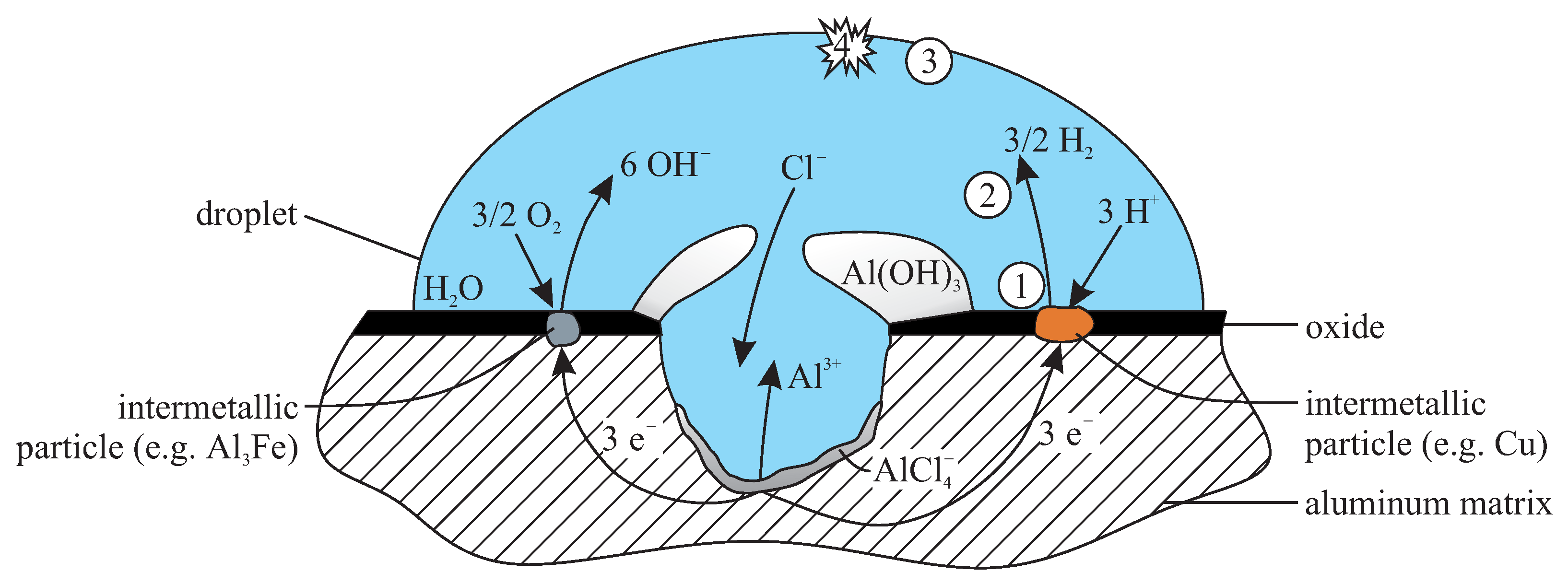
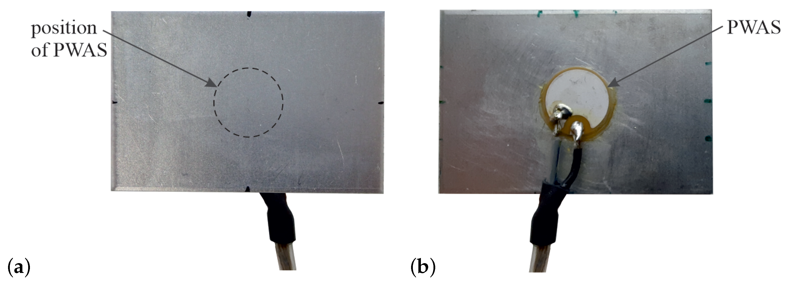
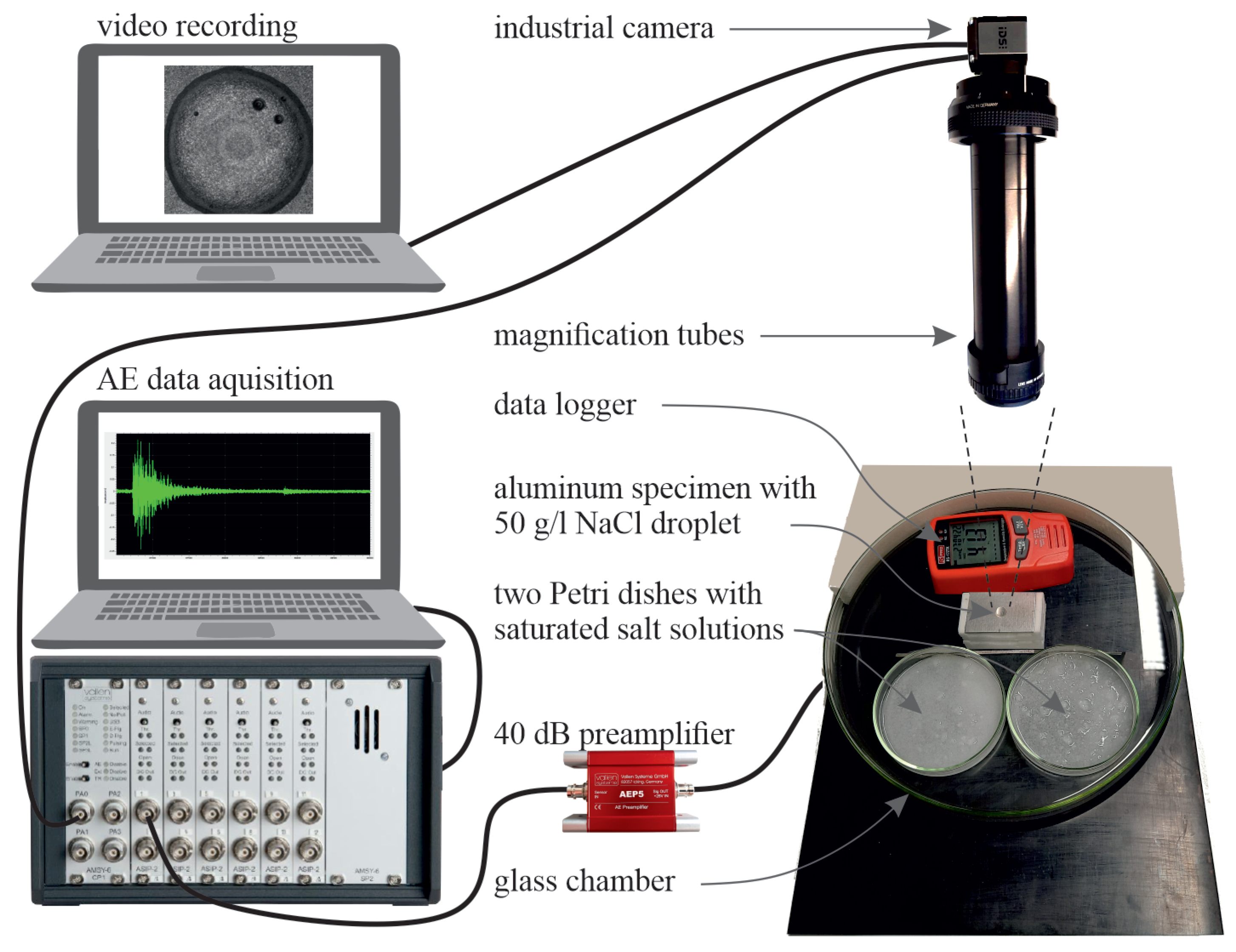
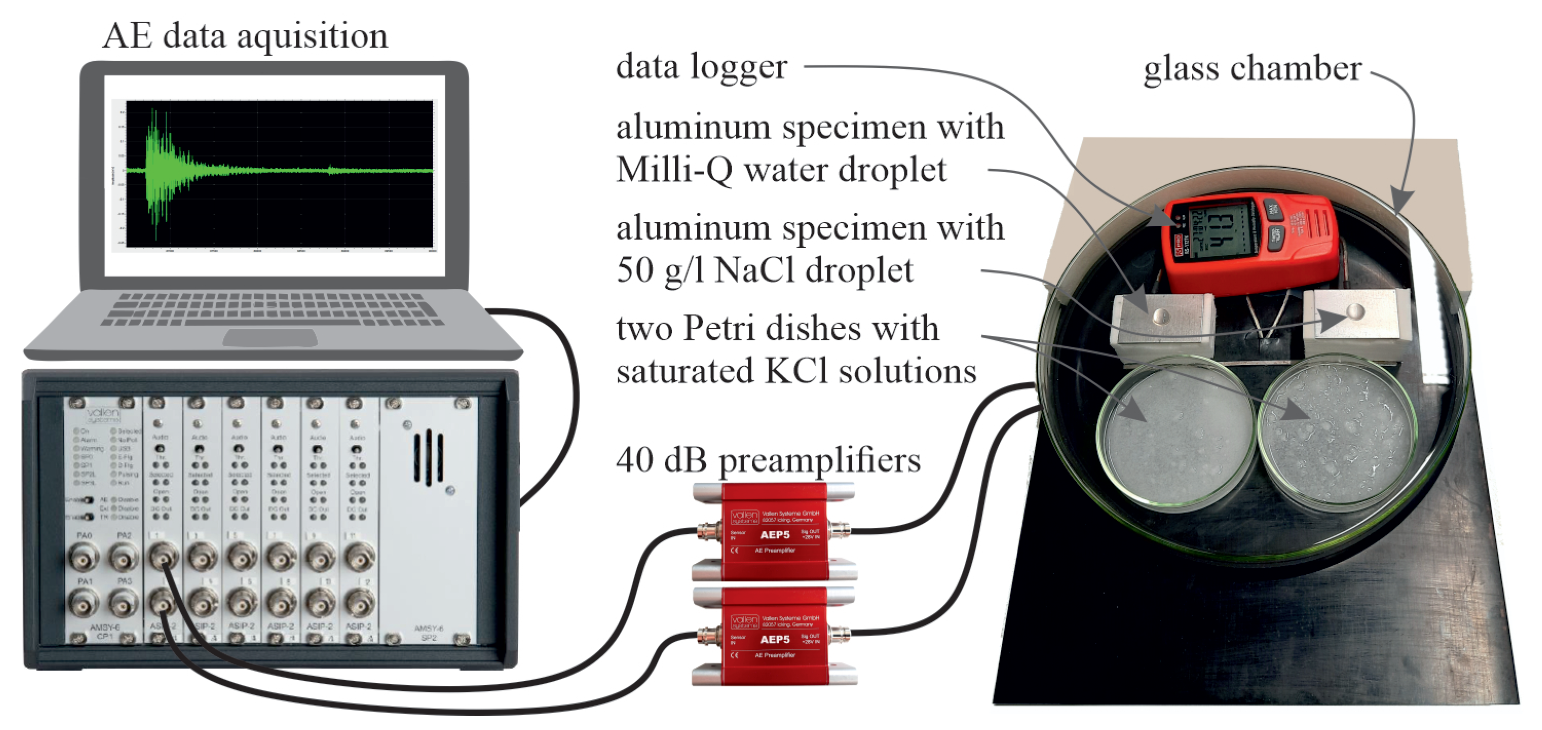
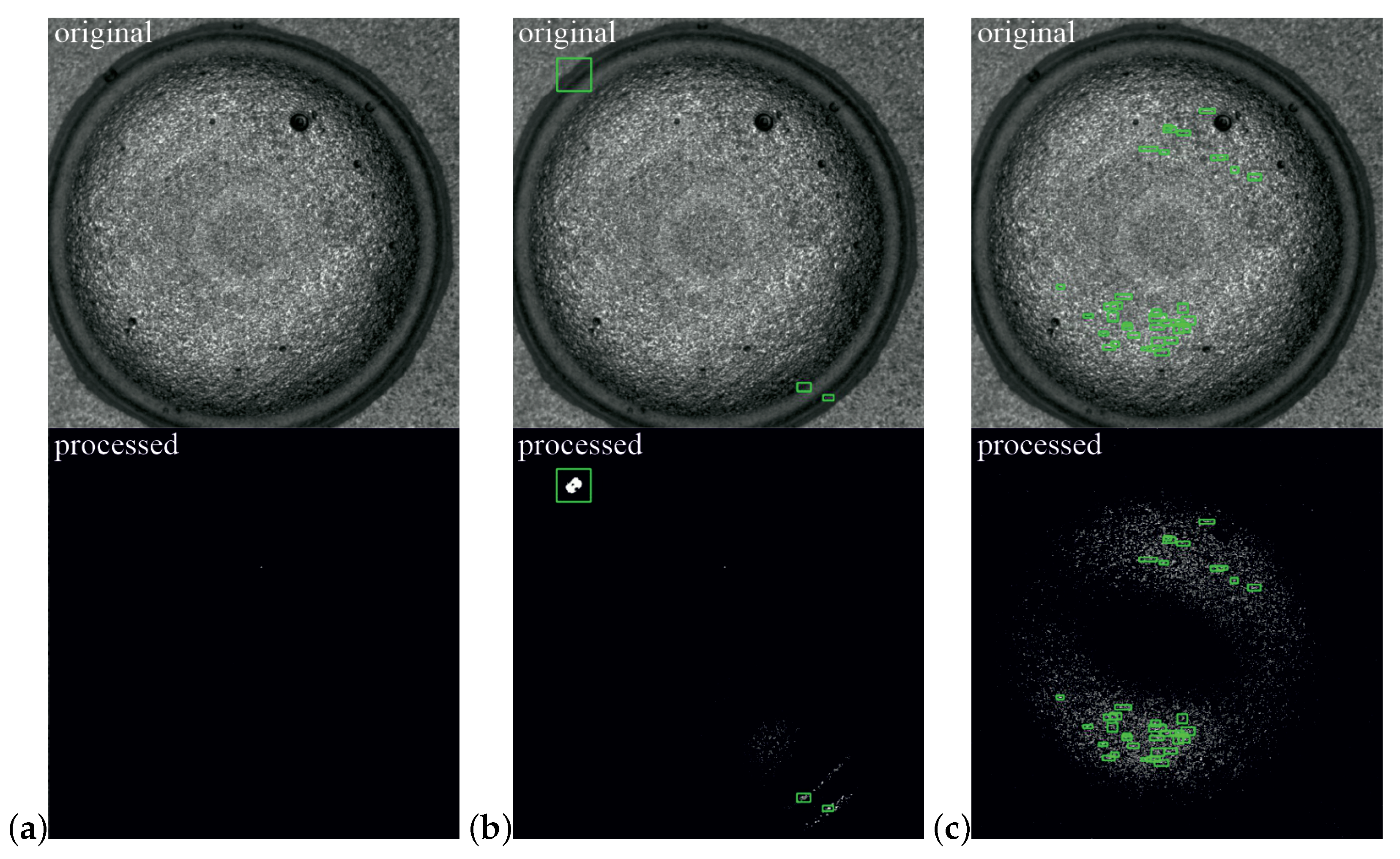
Table 1.
Salts required for the experiments described below, their purity and supplier, as well as their equilibrium relative humidity (RH) at 20 °C and 25 °C when used for the saturated salt solutions [31].
Table 1.
Salts required for the experiments described below, their purity and supplier, as well as their equilibrium relative humidity (RH) at 20 °C and 25 °C when used for the saturated salt solutions [31].
| Salt | Formula | Purity | Supplier | RH at 20 °C (%) | RH at 25 °C (%) |
|---|---|---|---|---|---|
| Magnesium chloride hexahydrate | MgCl2·6H2O | p.a. * | Merck | 33.0 | 32.5 |
| Magnesium nitrate hexahydrate | Mg(NO3)2·6H2O | p.a. * | Carl Roth | 55.0 | 53.0 |
| Sodium chloride | NaCl | ≥99.5% | Pharmasal | 76.0 | 75.5 |
| Potassium chloride | KCl | p.a. * | Carl Roth | 85.0 | 85.0 |
| Sodium sulfate decahydrate | Na2SO4·10H2O | p.a. * | Carl Roth | 93.0 | 93.0 |
* pro analysi.
Table 2.
Sequence of saturated solutions used to control the RH in the glass chamber.
| Step | Solution Petri Dish 1 | Solution Petri Dish 2 | Expected RH (%) | Remark |
|---|---|---|---|---|
| 0 | - | - | - | ambient RH |
| 1 | Na2SO4·10H2O | Na2SO4·10H2O | 93.0 | initial high RH |
| 2 | NaCl | NaCl | 76.0 | start of drying |
| 3 | NaCl | Mg(NO3)2·6H2O | 65.5 | - |
| 4 | Mg(NO3)2·6H2O | Mg(NO3)2·6H2O | 55.0 | - |
| 5 | MgCl2·6H2O | MgCl2·6H2O | 33.0 | - |
| 6 | Mg(NO3)2·6H2O | Mg(NO3)2·6H2O | 55.0 | start of rewetting |
| 7 | NaCl | NaCl | 76.0 | - |
| 8 | KCl | - | 85.0 | - |
| 9 | Na2SO4·10H2O | - | 93.0 | - |
| 10 | H2O | H2O | >93.0 | deionized water |
| 11 | silica gel | silica gel | <33.0 | final drying |
Disclaimer/Publisher’s Note: The statements, opinions and data contained in all publications are solely those of the individual author(s) and contributor(s) and not of MDPI and/or the editor(s). MDPI and/or the editor(s) disclaim responsibility for any injury to people or property resulting from any ideas, methods, instructions or products referred to in the content. |
© 2022 by the authors. Licensee MDPI, Basel, Switzerland. This article is an open access article distributed under the terms and conditions of the Creative Commons Attribution (CC BY) license (https://creativecommons.org/licenses/by/4.0/).
Share and Cite
MDPI and ACS Style
Erlinger, T.; Kralovec, C.; Schagerl, M. Monitoring of Atmospheric Corrosion of Aircraft Aluminum Alloy AA2024 by Acoustic Emission Measurements. Appl. Sci. 2023, 13, 370. https://doi.org/10.3390/app13010370
AMA Style
Erlinger T, Kralovec C, Schagerl M. Monitoring of Atmospheric Corrosion of Aircraft Aluminum Alloy AA2024 by Acoustic Emission Measurements. Applied Sciences. 2023; 13(1):370. https://doi.org/10.3390/app13010370
Chicago/Turabian StyleErlinger, Thomas, Christoph Kralovec, and Martin Schagerl. 2023. "Monitoring of Atmospheric Corrosion of Aircraft Aluminum Alloy AA2024 by Acoustic Emission Measurements" Applied Sciences 13, no. 1: 370. https://doi.org/10.3390/app13010370
Note that from the first issue of 2016, this journal uses article numbers instead of page numbers. See further details here.