
Consensus Cooperative Encirclement Interception Guidance Law for Multiple Vehicles against Maneuvering Target
by
 ,
,
Mingkun Guo
1,2 ,
,
Guangqing Xia
1,2,*,
Feng Yang
1,2,
Cong Liu
1,2,
Kai Liu
1,2 and
Jingnan Yang
1,2 1
State Key Laboratory of Structural Analysis for Industrial Equipment, School of Aeronautics and Astronautics, Dalian University of Technology, Dalian 116024, China
2
Key Laboratory of Advanced Technology for Aerospace Vehicles of Liaoning Province, School of Aeronautics and Astronautics, Dalian University of Technology, Dalian 116024, China
*
Author to whom correspondence should be addressed.
Appl. Sci. 2022, 12(14), 7307; https://doi.org/10.3390/app12147307
Submission received: 29 June 2022
/
Revised: 15 July 2022
/
Accepted: 16 July 2022
/
Published: 20 July 2022
(This article belongs to the Special Issue Intelligent Autonomous Decision-Making and Cooperative Control Technology of High-Speed Vehicle Swarms, Volume II)
Abstract
:This paper studies a cooperative encirclement interception guidance law against a maneuvering target that utilizes a leader–follower control scheme. The control design is decoupled into two parts. In the line-of-sight (LOS) direction, a fixed-time distributed disturbance observer is presented to estimate the maneuvering of the target. Based on the proposed disturbance observer, the guidance law is designed for the followers to guarantee that each follower’s total flight time achieves consensus with that of the leader. In the normal direction of the LOS, the control command is designed to realize the encirclement interception with a predefined-time consensus protocol. The convergence of the guidance algorithm is proven by the Lyapunov stability theory. Numerical simulations are provided to demonstrate the effectiveness and superiority of the proposed cooperative-guidance law.
1. Introduction
With the development of modern high-speed strike weapons, traditional one-to-one interception will face more difficulties against high-speed maneuvering targets. Multivehicle cooperative interception has received a great deal of attention. Compared with a single interceptor, cooperative simultaneous engagement can increase the interception coverage area and improve the interception probability. As one of the key technologies of cooperative engagement, the multivehicle cooperative interception guidance law has been a research hotspot in recent years. In previous studies, the cooperative-guidance law has mainly been divided into two parts: biased proportional navigation guidance [1,2,3], and multidirection-guidance [4,5]. However, some aspects of the guidance performance have yet to be improved, such as the maneuvering-target-capture ability and adaptive-control ability. Therefore, the multivehicle-cooperative-interception problem is of great significance.
The biased proportional-based guidance law originates from the individual homing guidance [6,7], in which the guidance law is designed individually, and the simultaneous engagement is reached by setting the same desired impact time for each interceptor in advance. Jeon et al. [6] designed an impact time control guidance (ITCG) law by biased proportional navigation guidance. Moreover, the biased term was designed as a time-error feedback form in the ITCG. As the earliest cooperative guidance method, ITCG laid the foundation for the biased proportional-based guidance law. The core of the biased proportional-based guidance law lies in the accurate estimate of the time-to-go under pure proportional guidance. Based on this, there are two directions that have mainly been studied. One is the improvement of the time-to-go estimation method. Jeon et al. [8] adjusted the time-to-go estimation form in 2016, which extended ITCG to nonlinear models, without the limitation of small-angle assumptions. Because of its simple form and high precision, the time-to-go estimation form in [8] is widely used. Wang et al. [9] estimated the time-to-go of a hypersonic vehicle with a new numerical method. Another direction is two-stage guidance. In the two-stage cooperative-guidance law, the second stage is generally designed as the form of the time-feedback-control proportional-guidance law, and the first stage is designed to provide the proper initial condition for the second-stage control. Common design approaches for the first stage include consistency control [10,11,12], trajectory shaping [13], and other advanced control methods [14,15]. It is worth mentioning that most time-to-go estimation forms are established on the basis of the constant-velocity hypothesis [8,16,17]. Moreover, most of the research on varying the velocity-time-estimation method is proposed based on uniform varying velocity [18,19]. These assumptions about the flight velocity reduce the applicable scope of the guidance law in real situations.
To solve the problem mentioned above, the multidirection-guidance method has been proposed in recent years. Similar to the traditional angle-constrained guidance law in line-of-sight (LOS) coordinate systems, a control in the normal direction of the LOS is designed to confirm the convergence of the LOS rate. Besides the control command in the normal direction of the LOS, the multidirection-guidance method adds the guidance law in the LOS direction to control the flight time. Therefore, the multidirection-guidance method can realize both the time constraint and the angle constraint. Consistency control is generally applied to guidance in the LOS direction. By exchanging information among vehicles via a communication network, the time-to-go of each vehicle can reach a consensus with a consensus protocol. Lin et al. [20] introduced the fixed-time control technique into the multidirection-guidance method to improve the convergence rate of the system. Zhou et al. [21] considered the data transmission in a discrete-time communication network. In order to adapt to this more realistic engagement situation, the time-estimation method was refined into a discretized form. However, the works proposed above focused on cooperative guidance against fixed targets or nonmaneuvering targets [6,7,8,9,10,11,12,13,14,15,16,17,18,19,20,21]. Less research has been conducted on cooperative guidance against maneuvering targets [22,23,24,25]. Dong et al. [22] designed an extended state observer (ESO) in both directions to estimate the uncertain disturbance caused by target maneuvers. In [23], to ensure the fast convergence of the time-to-go and reduce the impact of disturbances, super-twisting sliding-mode control was applied in LOS-direction guidance. Liang et al. [24] designed a fixed-time consensus protocol, which further improved the convergence rate of time. Cong et al. [25] proposed a distributed-model predictive-control-guidance law with the virtual-leader method to solve the three-dimensional cooperative-interception problem. Nevertheless, to the best of the authors’ knowledge, the multidirection-guidance method in the existing works controls the impact time individually. The impact angle of each vehicle is settled before launch, which prevents autonomous coordination.
As an effective tactic, encirclement guidance has received significant attention in recent years. Different methods have been proposed for surrounding the target from multiple angles. Yu et al. [26] propose a distributed cooperative encirclement hunting guidance law for multiple vehicles based on time-varying formation-tracking-control theories. However, the vehicles in [26] cannot attack the target simultaneously. In [27], encirclement interception for a fixed target is realized by a biased proportional-based guidance law.
In light of the aforementioned observations, this paper comes up with a novel cooperative-guidance law with a constrained impact angle and simultaneous attack. The main contributions of this paper are as follows:
- Compared with other cooperative-guidance laws [6,7,8,9,10,11,12,13,14,15,16,17,18,19,20,21] and encirclement-interception methods [27] that are aimed at a stationary target, this paper presents a new way to realize encirclement interception against a maneuvering target by utilizing a leader–follower topology. During the interception, the followers are arranged around the leader. The vehicles are separated by fixed LOS angles. The guidance law for the leaders is designed to intercept the target at a certain impact angle. Meanwhile, the cooperative guidance law for the followers is designed with variable LOS-angle constraints;
- A fixed-time distributed disturbance observer (DDOB) was designed to compensate for the insufficient target-maneuver information involved in the guidance law. Compared with the traditional disturbance observer in [22], our distributed disturbance observer has a better performance in distributed cooperative interception;
- A predefined-time consensus guidance (PTCG) law was designed to control the impact angle of the vehicles. Compared with [22,23,24,25], the proposed PTCG introduces the communication-consistency control into the guidance law in the normal direction of the LOS, which improves the adaptive-control ability. Furthermore, the proposed PTCG can ensure that the LOS angles of the followers converge to the desired values in the prescribed time. The convergence time is set as the total flight time, which reduces the control input saturation.
The remainder of this paper is organized as follows. Some necessary preliminary knowledge is provided in Section 2. The problem formulation is presented in Section 3. Section 4 presents the design of our cooperative-guidance law and the stability analysis. Numerical simulations are provided in Section 5 to demonstrate its effectiveness and superiority. Finally, conclusions are presented in Section 6.
2. Preliminaries
This section provides a brief introduction to graph theory, ESO theory, finite-time convergence theory, and fixed-time convergence theory.
2.1. Some Key Definitions
To posit the surrounding interception problem, a few terminologies need to be defined.
An extended state observer (ESO) [28] is a state observer that comes up against an uncertainty estimation. It is the key link toward the active disturbance-rejection control. Through the ESO, we are able to cancel the total disturbance in the design of the controller.
The time to go () [29] is defined as the time that remains for each vehicle to intercept the target. If is the time of interception, then , where t is the present time. Both t and are defined with respect to the same reference.
2.2. Graph Theory
Suppose that there are N vehicles participating in a cooperative-attack mission. The information communication among multiple vehicles can be described with an interaction digraph [22]. Let G (M, E, A) denote a communication graph. G (M, E, A) consists of a node (), an edge (), and the weighted adjacency matrix (). The adjacency element () satisfies if and only if information is exchanged between and . If there is a directed path between any two distinct nodes, the directed graph is strongly connected. The in-degree of the node () is defined as . The diagonal matrix obtained from the as diagonal entries is called the diagonal in-degree matrix (D). Finally, the graph Laplacian matrix is obtained as . The Laplacian matrix () of the directed graph (G) is defined by:
where denotes the fields of real numbers.
2.3. ESO Theory
Lemma 1.
whereis the state variable,is the control input, andis the uncertainty disturbance. Ifis bounded, one can denoteas an extended state. The ESO [30] can be modeled a:
whereis the estimation of states. Withbeing a proper vector, the estimation error () could be arbitrarily small.
Consider the high-order nonlinear system:
2.4. Finite-Time Convergence Theory
Lemma 2.
where.
Consider a nonlinear control system:
Suppose there exists a continuous, differentiable, positive definite, and radially unbounded function: , . The origin of the system (4) is a globally finite-time convergent equilibrium when it satisfies [31]:
where , and the settling-time function satisfies:
2.5. Fixed-Time Convergence Theory
Lemma 3.
where, and the settling-time function satisfies:
Consider a nonlinear control system (4). Suppose there exists a continuous, differentiable, positive definite function: , . The origin of the system (4) is a fixed-time convergent equilibrium if it is a finite-time convergent equilibrium [31] and:
Notations.
Define the function by if , and by if . Define .
3. Problem Formulation
In this paper, the combat scenario of multiple 2D vehicles intercepting a maneuvering target is studied. The goal is to simultaneously intercept the target by deploying multiple interceptors. Consider a group of N intercepting vehicles: , denote the interceptors and T denotes the target. The planar one-to-one engagement between the interceptor and a target may be depicted as in Figure 1. Both the interceptors and the target are assumed to be point masses, and their velocity vectors are denoted by and , respectively. Moreover, the corresponding speeds of them ( and , respectively) are constants. Their LOS angles are and , respectively. The flight path angles are and , respectively. The term denotes the distance between the vehicle () and the target (T). The relative separation between the target and the interceptor and the LOS angle are denoted by and , respectively:
In an interception scenario, according to the principles of kinematics, the relative-motion equation can be deduced as:
To guarantee a salvo attack of the target by multiple interceptors, it is desirable that the interceptors achieve agreement on the time-to-go. Furthermore, this paper provides an encirclement-guidance strategy by utilizing a leader–follower topology. Considering N interceptors containing one leader and N − 1 followers, the vehicles can exchange information with communication networks, expressed by the weighted adjacency matrix: . The guidance geometry is illustrated in Figure 2. Let denote the leader, and , denote the followers. The directed communication link is described by the blue arrows:
Note 1.
As is shown in Figure 2, the leader and followers play different roles in the communication topology. The leader can send guidance information to adjacent followers. Each follower can work as an information transfer station. The mathematical models for the leader and followers are different, and the guidance laws for the leader and followers should be designed accordingly.
The derivatives of (9) and (10) can be obtained as:
The motion equations in the LOS direction and its normal are given by (13) and (14), where and denote the components of the acceleration of the interceptor and the target in the LOS direction, respectively. and denote the components of the acceleration of the interceptor and the target in the normal direction of the LOS, respectively.
In order for multiple vehicles to simultaneously attack the target at preset angles, the following nonlinear state equation is now established. Define the state variables as , , , , , where denotes the desired terminal LOS angle.
When , the interceptor is the leader, and is a predefined constant. There is no need to design control command in the LOS direction. The cooperative-guidance model can be described as:
When , the interceptor is the follower. To maintain the encirclement-interception formation, the is connected with the other interceptors:
where denotes the LOS angle error of the encirclement interception. Then, the cooperative-guidance model changes as follows:
where .
During the interception process, the time-to-go of the interceptor can be approximated by:
By taking the derivate of (18), we obtain the following:
A new state-variable flight time () is introduced as follows:
Define the error of the flight time:
Taking the derivative of (21) yields:
To realize simultaneous arrival, we introduce the new state variable (), and the cooperative-guidance model for the followers (17) can be rewritten as:
Remark 1.
Our cooperative-guidance law aims to arrange the followers around the leader to realize the encirclement attack. The separation distance between different vehicles is designed by the LOS angle error (). Unlike the traditional cooperative-guidance law with the static LOS-angle constraint in [22,23,24,25], our guidance law sets the various LOS angle constraints for the followers, which adaptively adjust to the LOS angle of the leader and the LOS angle error. This cooperative-encirclement-guidance strategy brings a new differential term: . This term can be obtained by the communication with the other interceptors.
4. Main Results
In this section, to realize the encirclement-interception-control objective, the cooperative-guidance problem is divided into two parts: the flight-time control part and the impact-angle control part. The flight-time control part is designed in the LOS direction. In this part, only the guidance law of the followers is designed. The main objective is to achieve consistent timing for the leader and followers under the distributed communication structure. In the normal direction of the LOS, the guidance laws of the leader and followers are designed accordingly: the guidance law for the leader is designed to attack the target at a specific angle, and the guidance law for the followers is designed to form the ring of encirclement.
4.1. Flight-Time Control Part
In this part, the guidance law for the followers in the LOS direction is designed to realize simultaneous arrival. Equation (17) shows that there is an uncertain disturbance caused by the target maneuver. Designing a disturbance observer to estimate the maneuver of the target is the first step. In light of [30] and the ESO theory in Lemma 1, a fixed-time distributed disturbance observer (DDOB) is presented as follows: Let denote the estimation of the consensus error of the between multiple vehicles, and let denote the estimation of the uncertain disturbance. Then, the observer is designed as follows:
Moreover, , satisfies , .
Theorem 1.
For system (22), with the fixed-time distributed observer (24), assuming that and are known and the disturbance caused by the target satisfies the boundary condition, , where is finite and unknown, the observation error of and will converge to a neighborhood of the origin in fixed time. The result of the contrast is shown inSection 5.
Proof of Theorem 1.
The proof is provided in Appendix A. □
Remark 2.
Because of the special distributed model (23) in the followers’ cooperative-guidance law, the traditional fixed-time disturbance observer (FxTDO) is no longer effective. To solve this problem, we proposed the DDOB. As is shown in (24), the state variables that Z1tracks are designed as a distributed form () by the communication graph. Compared with the other single-vehicle disturbance observer methods [23,32], our DDOB is more suitable for multivehicle-cooperative-combat environments.
Theorem 2.
The system can converge to zero within a finite time by the guidance law as:
whereand.
Under the undirected graph, consider a one-order system as follows:
Proof of Theorem 2.
The proof is provided in Appendix B. □
Theorem 3.
If the undirected graph of the multivehicle system is connected, the impact time of all the missiles will converge to the same value within a finite time with the guidance law:
Proof of Theorem 3.
By combining (28) with (23), one can obtain:
By utilizing Theorem 2, can converge to zero in finite time. This indicates that the total flight time of the followers can remain consistent, and furthermore, that it can be consistent with that of the leader. □
Remark 3.
In (28), the cooperative-guidance law for the followers does not require precise target-maneuver information. The uncertain disturbance term () in (23) that is caused by the target maneuver is compensated for by the DDOB. When the target maneuver is within a certain limit, our guidance law can realize the control objective.
4.2. Impact-Angle Control Part
In the impact control part, the guidance laws for the leader and followers are designed accordingly. First, the nonsingular terminal sliding-mode guidance law [33] for the leader is presented. Consider the sliding-mode surface:
where , . Based on (30), a finite-time convergence guidance law can be designed as:
where , and .
Then, in light of the study in [34], a novel predefined-time consensus guidance law is proposed so that the followers simultaneously attack the target at the desired impact angle. A time-varying sliding-mode surface is designed as follows:
where . Moreover, a predefined-time guidance law is designed as:
Theorem 4.
In the second-order nonlinear system (23), if the guidance law is designed as in (33), then the state variables and will simultaneously converge to zero at .
Proof of Theorem 4.
The proof is provided in Appendix C. □
Note 2.
where is a constant.
In (33), the discontinuous control term () is designed to compensate for the target maneuver in normal LOS directions. However, the discontinuous control term may cause control-input chattering. In the numerical simulations, we used an approximate function to obtain continuous guidance commands, as follows:
Remark 4.
As is shown in (33), the convergence time of the rate of the LOS in the proposed PTCG is designed as the , which means that the attack angle will converge to the expected value exactly when the interception impact appears. It is worth noting that the convergence time can be adjusted by replacing with the convergence time (). The convergence time () can be predetermined arbitrarily and independently of the system parameters or constants. This is the main superiority of the predefined-time guidance law.
Remark 5.
The existing study [35] on the predefined-time cooperative-guidance law focuses on its effectiveness at avoiding collisions between interceptors by the rapid convergence of the LOS. However, previous guidance laws, such as the finite-time cooperative-guidance law [23] and fixed-time cooperative-guidance law [20], can guarantee the rapid convergence of the rate of the LOS. Compared with such methods [20,23], there is no significant advantage with the predefined-time cooperative-guidance law. In this paper, the superiority of the predefined-time cooperative-guidance law is applied to reduce the saturation of the control input. A controllable slower convergence rate is realized without the parameter design. Moreover, PTCG reduces the step of designing the reasonable convergence time. These factors facilitate the engineering realization.
5. Numerical Simulations
In this section, numerical simulations are given to demonstrate the effectiveness and superiority of the proposed cooperative-guidance law. Consider the situation in which five vehicles simultaneously intercept a maneuvering target. The initial conditions of the multiple vehicles and target are presented in Table 1. Due to the physical constraints of the vehicles, the maximum accelerations in all directions are limited to 25 g, where g denotes the gravitational acceleration, and . The attack angle of the leader is set as 10°. To realize the encirclement interception, the followers are arranged on both sides of the leader with 15 degrees attack angles apart.
The communication topology of the vehicles is shown in Figure 3.
The initial conditions of the target are shown in Table 2.
The control parameters are designed as follows:
The simulation results with our guidance law are exhibited in Figure 4, Figure 5, Figure 6, Figure 7, Figure 8 and Figure 9. From Figure 4, it can be observed that the multiple vehicles can intercept the maneuvering target along different trajectories. Figure 5 shows the time-to-go of the interceptors. To further demonstrate the convergence process, the tracking error between the followers and leader is provided in picture-in-picture. The of each follower converges to the value of the leader rapidly, which means that the cooperative attack has been completed. Figure 6 shows that the vehicles attack the target with the different desired angles, and that the predetermined encirclement tactics can be implemented. Figure 7 gives the control command in the LOS direction during the engagement. The control command in the LOS direction is used to adjust the of the multiple vehicles. In Figure 8, owing to the initial attack-angle errors of the vehicles, the control commands in the normal direction of the LOS are relatively large at the beginning of the guidance. As is shown in Figure 9, the flight speeds of the five vehicles are constantly adjusted within a relatively small range. In the initial phase of the flight, a large overload is applied in the normal direction of the LOS to control the attack angle, which leads to an increase in the speeds of the multiple vehicles. Meanwhile, the overload in the direction of the LOS is applied to track the flight time of the leader, as well as to compensate for the normal overload. With the rapid convergence of the attack angle and flight time, the control overloads tend to be gentle. The variation in the speeds of the multiple vehicles tends to be stable.
The estimation performance of our fixed-time distributed disturbance observer is shown in Figure 10 and Figure 11. It can be seen that the disturbance error of the DDOB can converge to the neighborhood of the origin in time.
To validate the superiority of the proposed cooperative-guidance law, a series of contrast experiments were presented as follows. The comparison between our guidance law and the finite-time consensus-guidance (FTCG) law based on finite-time control [36] without the DDOB is shown in Figure 12. Owing to the maneuver of the target, the control commands of the followers in the LOS direction will change rapidly when the interceptors are closed to the target. The proposed DDOB can significant decrease the effect caused by the uncertain disturbance. In Figure 13, an estimation simulation with an ESO based on the disturbance observer in [22] is carried out for comparison. It can obviously be seen that large saturation shocks are avoided by using the DDOB.
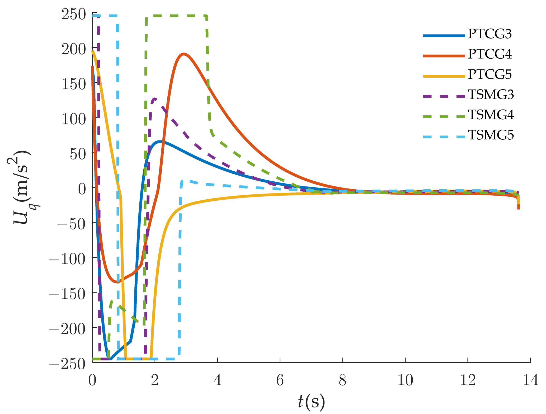
Figure 14 and Figure 15 show the superiority of the proposed predefined-time guidance law compared with the terminal sliding-mode guidance (TSMG) law [4]. In Figure 14, the attack angles of the interceptors under PTCG converge more gently than those under TSMG. To make the display clearer, we chose to compare Vehicle 2, Vehicle 3, and Vehicle 4 as an example in Figure 15. This can avoid the large overloads on the interceptors for a long period of time at the beginning of the guidance.
6. Conclusions
This study is concerned with the cooperative-encirclement-interception problem for multiple vehicles against a maneuvering target, with consideration to communication networks. To realize the simultaneous encirclement interception, we divided the guidance into two parts. In the flight-control part, a distributed disturbance observer is proposed. Based on the finite-time consistency theory and the fixed-time distributed disturbance observer, a consensus-guidance law is designed in the LOS direction. Meanwhile, in the impact-angle control part, a predefined-time guidance law is designed with a time-varying sliding mode. The effectiveness and superiority of the proposed methods are verified by simulations. In future works, we will extend our algorithm to the three-dimensional guidance law.
Author Contributions
Conceptualization, M.G. and G.X.; methodology, M.G.; software, F.Y.; validation, C.L. and J.Y.; formal analysis, F.Y.; investigation, G.X.; resources, K.L.; data curation, M.G.; writing—original draft preparation, M.G.; writing—review and editing, J.Y.; visualization, C.L.; supervision, G.X.; project administration, F.Y.; funding acquisition, K.L. All authors have read and agreed to the published version of the manuscript.
Funding
The research was funded by the National Natural Science Foundation of China, grant number (U2141229), and by the Aeronautical Science Foundation, grant number (2019ZC063001).
Institutional Review Board Statement
Not applicable.
Informed Consent Statement
Not applicable.
Data Availability Statement
The data presented in this study are available upon request from the corresponding author.
Conflicts of Interest
The authors declare no conflict of interest.
Appendix A
Introduce the definitions as follows:
Define the unknown disturbance as follows:
By substituting (A1) into (24), one obtains:
Let , and .
Step 1. Suppose the disturbance of (22) is zero, define:
If (A4) is in the dominant scope of the low-order power function, then (i.e., ). If (A4) is in the dominant scope of the high-order power function, then (i.e., ). Thus, no matter what the value of is, and are continuous. According to the Definitions (4–6) in [37], the function is homogeneous in both the 0-limit and -limit.
Because and satisfy and , based on the work in [38], the origins of and are globally asymptotically stable if their polynomials are Hurwitz. Moreover, the origin of the system () is asymptotically stable if the polynomials are Hurwitz. To allow all the roots of these polynomials in the negative real axis, the value of should be large enough and should satisfy:
Let the real numbers and satisfy:
It is known that , and are globally asymptotically stable, according to Definition 5 in [30]. There exists a continuously differentiable, positive definite, and radially unbounded Lyapunov function ( of ), which is homogeneous in the bilimit with associated triples: and . In addition, is negative definite and homogeneous in the bilimit with associated triples: and .
Define the following functions:
where is homogeneous in the bilimit with associated triples: and . is homogeneous in the bilimit with the weights and , and the degrees and . On the basis of Lemma 1 in [30], for , there exists:
Then, we can obtain:
because:
Function (A9) can be reduced as:
According to Lemma 3, it can be deduced that:
Step 2. Suppose the disturbance of (A3) is not zero, according to the Lyapunov function provided in [36], the differential of can be obtained as follows, along (A3):
where is homogeneous in the bilimit with associated triples: and , and .
Define the functions:
where is homogeneous in the bilimit with associated triples: and . is homogeneous in the bilimit with associated triples: and .
On the basis of Lemma 1 in [30], for , there exists:
By substituting (A15) into (A14), one can obtain:
where , and . Then, (A16) can be simplified into:
By substituting (A9) and (A17) into (A13), we can obtain:
Rewrite (A18) as follows:
where (A19) represents the Lyapunov inequality if the high-order power term is dominant, and (A20) represents the Lyapunov inequality if the low-order power term is dominant. Considering:
one can deduce that:
Because of , (A22) can be rewritten as follows:
When , we can obtain the following from (A19):
Then, the convergence time () from to is:
In other words, is the finite-time () convergent to the neighborhood () of the origin, where:
and .
When , we can obtain the following from (A20):
Then, the convergence time () from to is:
In other words, is the finite-time () convergent to the neighborhood () of the origin, where:
and .
Hence, is the fixed-time convergent to a neighborhood of the origin. The convergence time is presented in (A25) and (A28), and the convergence domain is presented in (A26) and (A29). By , the observation error of and will converge to a neighborhood of the origin in a fixed time. This completes the proof of Theorem 1.
Appendix B
Consider the following Lyapunov function:
Take the derivative of (A30), and then:
According to Lemma 2, the system (26) will converge to zero in finite time. Then, we have:
This completes the proof of Theorem 2.
Appendix C
Consider the following Lyapunov function:
By taking the derivative of (32), one can obtain:
By taking the derivative of (A34), then:
Define as the uncertain disturbance (). Then, (A36) comes to:
Therefore, the sliding surface () can converge to zero. When is achieved, we can deduce that:
To simplify the calculation, define , and then:
It can be observed that the solution to (A39) is given as:
where:
From (A40), one can obtain:
Taking the derivative of (A42), we can obtain:
From (A42) and (A43), one can further obtain:
This completes the proof of Theorem 4.
References
- Zhu, C.H.; Xu, G.D.; Wei, C.Z.; Cai, D.Y.; Yu, Y. Impact-Time-Control Guidance Law for Hypersonic Missiles in Terminal Phase. IEEE Access 2020, 8, 44611–44621. [Google Scholar] [CrossRef]
- Tang, Y.; Zhu, X.P.; Zhou, Z.; Yan, F. Two-phase guidance law for impact time control under physical constraints. Chin. J. Aeronaut. 2020, 33, 2946–2958. [Google Scholar] [CrossRef]
- Cho, N.; Kim, Y. Modified Pure Proportional Navigation Guidance Law for Impact Time Control. J. Guid. Control Dyn. 2016, 39, 852–872. [Google Scholar] [CrossRef]
- Song, J.; Song, S.; Xu, S. Three-dimensional cooperative guidance law for multiple missiles with finite-time convergence. Aerosp. Sci. Technol. 2017, 67, 193–205. [Google Scholar] [CrossRef]
- An, K.; Guo, Z.-Y.; Huang, W.; Xu, X.-P. A Cooperative Guidance Approach Based on the Finite-Time Control Theory for Hypersonic Vehicles. Int. J. Aeronaut. Space Sci. 2022, 23, 169–179. [Google Scholar] [CrossRef]
- Jeon, I.S.; Lee, J.I.; Tahk, M.J. Impact-time-control guidance law for anti-ship missiles. IEEE Trans. Control Syst. Technol. 2006, 14, 260–266. [Google Scholar] [CrossRef]
- Jeon, I.-S.; Lee, J.-I.; Tahk, M.-J. Homing Guidance Law for Cooperative Attack of Multiple Missiles. J. Guid. Control Dyn. 2010, 33, 275–280. [Google Scholar] [CrossRef]
- Jeon, I.-S.; Lee, J.-I.; Tahk, M.-J. Impact-Time-Control Guidance with Generalized Proportional Navigation Based on Nonlinear Formulation. J. Guid. Control Dyn. 2016, 39, 1885–1890. [Google Scholar] [CrossRef]
- Wang, J.; Zhang, R. Terminal Guidance for a Hypersonic Vehicle with Impact Time Control. J. Guid. Control Dyn. 2018, 41, 1790–1798. [Google Scholar] [CrossRef]
- Zhang, Y.; Tang, S.; Guo, J. Two-stage cooperative guidance strategy using a prescribed-time optimal consensus method. Aerosp. Sci. Technol. 2020, 100, 105641. [Google Scholar] [CrossRef]
- He, S.; Wang, W.; Lin, D.; Lei, H. Consensus-Based Two-Stage Salvo Attack Guidance. IEEE Trans. Aerosp. Electron. Syst. 2018, 54, 1555–1566. [Google Scholar] [CrossRef]
- Zhao, Q.; Dong, X.; Liang, Z.; Bai, C.; Chen, J.; Ren, Z. Distributed cooperative guidance for multiple missiles with fixed and switching communication topologies. Chin. J. Aeronaut. 2017, 30, 1570–1581. [Google Scholar] [CrossRef]
- Zeng, J.; Dou, L.; Xin, B. A joint mid-course and terminal course cooperative guidance law for multi-missile salvo attack. Chin. J. Aeronaut. 2018, 31, 1311–1326. [Google Scholar] [CrossRef]
- Hu, Q.L.; Han, T.; Xin, M. New Impact Time and Angle Guidance Strategy via Virtual Target Approach. J. Guid. Control Dyn. 2018, 41, 1755–1765. [Google Scholar] [CrossRef]
- Ai, X.; Wang, L.; Yu, J.; Shen, Y. Field-of-view constrained two-stage guidance law design for three-dimensional salvo attack of multiple missiles via an optimal control approach. Aerosp. Sci. Technol. 2019, 85, 334–346. [Google Scholar] [CrossRef]
- Zhao, J.; Yang, S. Integrated cooperative guidance framework and cooperative guidance law for multi-missile. Chin. J. Aeronaut. 2018, 31, 546–555. [Google Scholar] [CrossRef]
- Dhananjay, N.; Ghose, D. Accurate Time-to-Go Estimation for Proportional Navigation Guidance. J. Guid. Control Dyn. 2014, 37, 1378–1383. [Google Scholar] [CrossRef]
- Jia, S.; Wang, X.; Li, F.; Wang, Y. Distributed Analytical Formation Control and Cooperative Guidance for Gliding Vehicles. Int. J. Aerosp. Eng. 2020, 2020, 8826968. [Google Scholar] [CrossRef]
- Sun, G.; Wen, Q.; Xu, Z.; Xia, Q. Impact time control using biased proportional navigation for missiles with varying velocity. Chin. J. Aeronaut. 2020, 33, 956–964. [Google Scholar] [CrossRef]
- Lin, M.; Ding, X.; Wang, C.; Liang, L.; Wang, J. Three-Dimensional Fixed-Time Cooperative Guidance Law With Impact Angle Constraint and Prespecified Impact Time. IEEE Access 2021, 9, 29755–29763. [Google Scholar] [CrossRef]
- Zhou, J.; Wu, X.; Lv, Y.; Wen, G. Terminal-time synchronization of multiple vehicles under discrete-time communication networks with directed switching topologies. IEEE Trans. Circuits Syst. II Express Briefs 2019, 67, 2532–2536. [Google Scholar] [CrossRef]
- Dong, X.; Ren, Z. Impact angle constrained distributed cooperative guidance against maneuvering targets with undirected communication topologies. IEEE Access 2020, 8, 117867–117876. [Google Scholar] [CrossRef]
- Zhang, S.; Guo, Y.; Liu, Z.; Wang, S.; Hu, X. Finite-Time Cooperative Guidance Strategy for Impact Angle and Time Control IEEE Trans. Aerosp. Electron. Syst. 2021, 57, 806–819. [Google Scholar] [CrossRef]
- Jing, L.; Wei, C.; Zhang, L.; Cui, N. Cooperative Guidance Law with Predefined-Time Convergence for Multimissile Systems. Math. Probl. Eng. 2021, 2021, 9940240. [Google Scholar] [CrossRef]
- Cong, M.; Cheng, X.; Zhao, Z.; Li, Z. Studies on Multi-Constraints Cooperative Guidance Method Based on Distributed MPC for Multi-Missiles. Appl. Sci. 2021, 11, 10857. [Google Scholar] [CrossRef]
- Yu, J.; Dong, X.; Li, Q.; Ren, Z. Distributed cooperative encirclement hunting guidance for multiple flight vehicles system. Aerosp. Sci. Technol. 2019, 95, 105475. [Google Scholar] [CrossRef]
- Yan, P.P.; Fan, Y.H.; Liu, R.F.; Wang, M.G. Distributed target-encirclement guidance law for cooperative attack of multiple missiles. Int. J. Adv. Robot. Syst. 2020, 17, 1–15. [Google Scholar] [CrossRef]
- Guo, B.Z.; Zhao, Z.L. On the convergence of an extended state observer for nonlinear systems with uncertainty. Syst. Control Lett. 2011, 60, 420–430. [Google Scholar] [CrossRef]
- Kumar, S.R.; Mukherjee, D. Deviated pursuit-based nonlinear cooperative salvo guidance using finite-time consensus. Nonlinear Dyn. 2021, 106, 605–630. [Google Scholar] [CrossRef]
- Yang, F.; Wei, C.-Z.; Wu, R.; Cui, N.-G. Non-recursive fixed-time convergence observer and extended state observer. IEEE Access 2018, 6, 62339–62351. [Google Scholar] [CrossRef]
- Polyakov, A. Nonlinear feedback design for fixed-time stabilization of linear control systems. IEEE Trans. Autom. Control 2011, 57, 2106–2110. [Google Scholar] [CrossRef] [Green Version]
- Zhang, P.; Zhang, X. Multiple missiles fixed-time cooperative guidance without measuring radial velocity for maneuvering targets interception. ISA Trans. 2022, 126, 388–397. [Google Scholar] [CrossRef]
- Yang, F.; Xia, G. A finite-time 3D guidance law based on fixed-time convergence disturbance observer. Chin. J. Aeronaut. 2020, 33, 1299–1310. [Google Scholar] [CrossRef]
- Pal, A.K.; Kamal, S.; Yu, X.; Nagar, S.K.; Xiong, X. Free-Will Arbitrary Time Consensus for Multiagent Systems. IEEE Trans. Cybern. 2020, 52, 4636–4646. [Google Scholar] [CrossRef]
- Wang, Z.; Fu, W.; Fang, Y.; Zhu, S.; Wu, Z.; Wang, M. Prescribed-time cooperative guidance law against maneuvering target based on leader-following strategy. ISA Trans. 2022. [Google Scholar] [CrossRef]
- Polyakov, A.; Fridman, L. Stability notions and Lyapunov functions for sliding mode control systems. J. Frankl. Inst. 2014, 351, 1831–1865. [Google Scholar] [CrossRef] [Green Version]
- Wu, R.; Wei, C.; Yang, F.; Cui, N.; Zhang, L. FxTDO-based non-singular terminal sliding mode control for second-order uncertain systems. IET Control Theory Appl. 2018, 12, 2459–2467. [Google Scholar] [CrossRef]
- Basin, M.; Yu, P.; Shtessel, Y. Finite-and fixed-time differentiators utilising HOSM techniques. IET Control Theory Appl. 2017, 11, 1144–1152. [Google Scholar] [CrossRef]
Figure 1.
Planar one-to-one engagement.

Figure 2.
Encirclement salvo attack engagement.
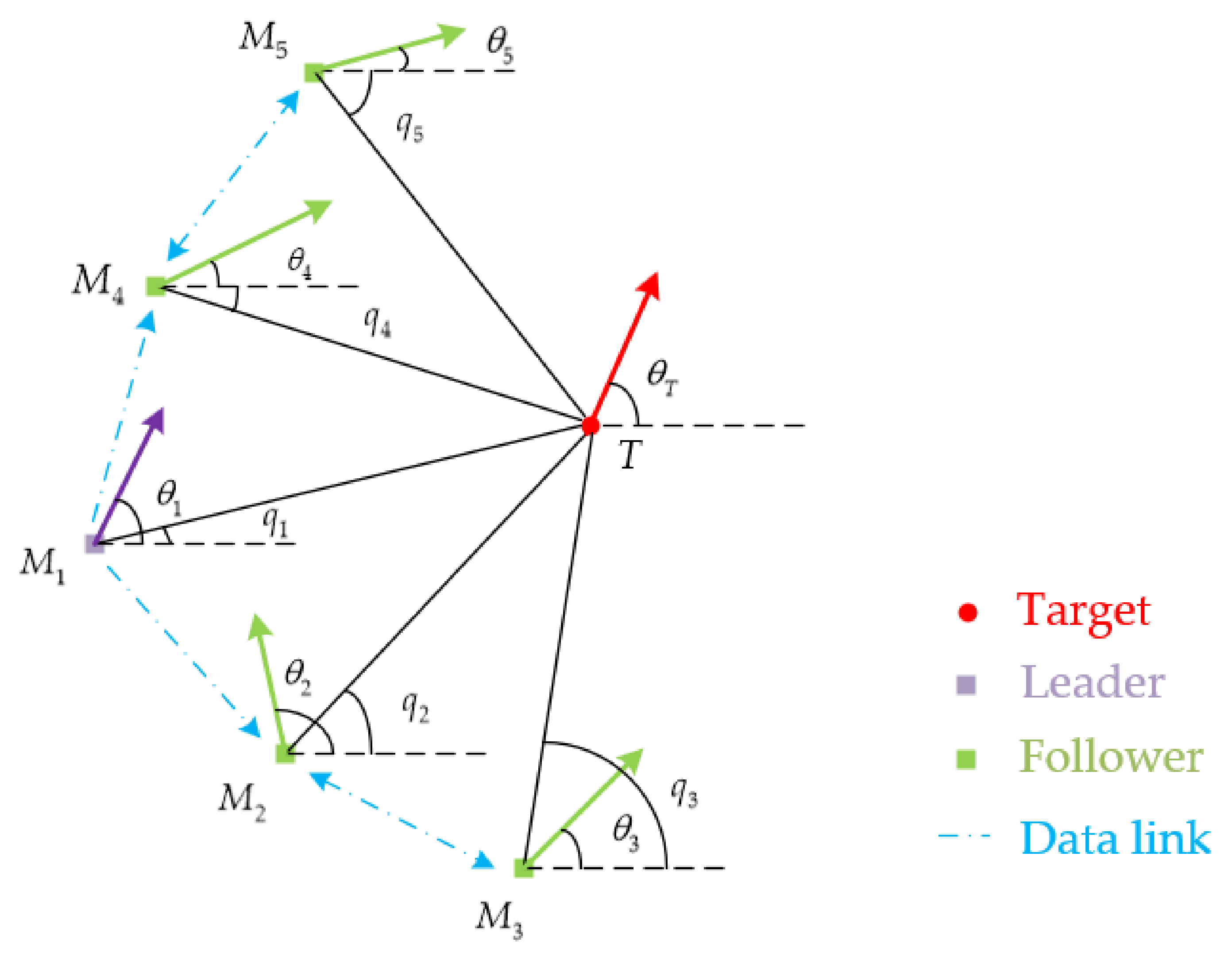
Figure 3.
Communication topology of vehicles.

Figure 4.
Trajectories of the vehicles and target.
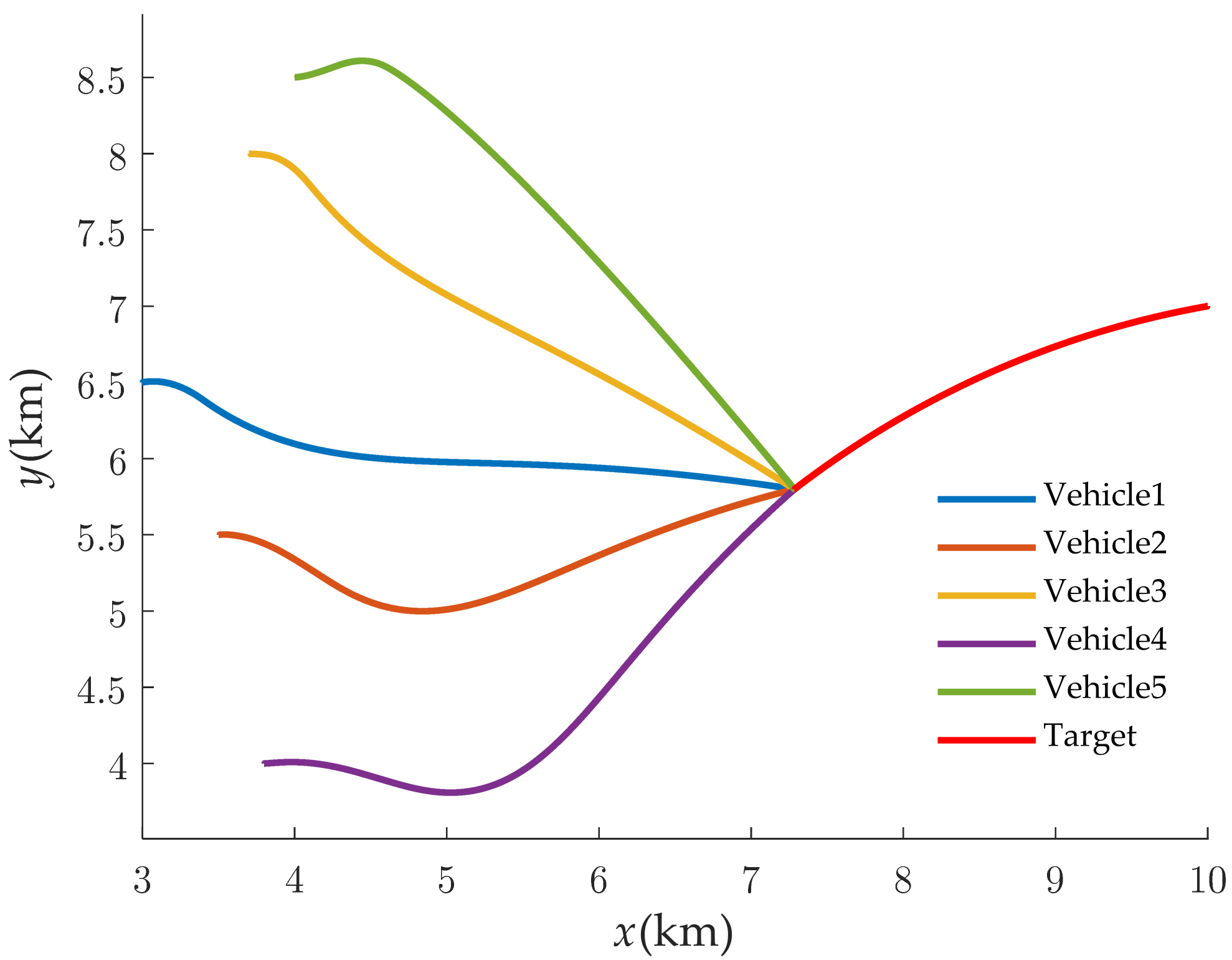
Figure 5.
Time-to-go of multiple vehicles.

Figure 6.
Attack angles of the LOS.

Figure 7.
Control commands in LOS direction.
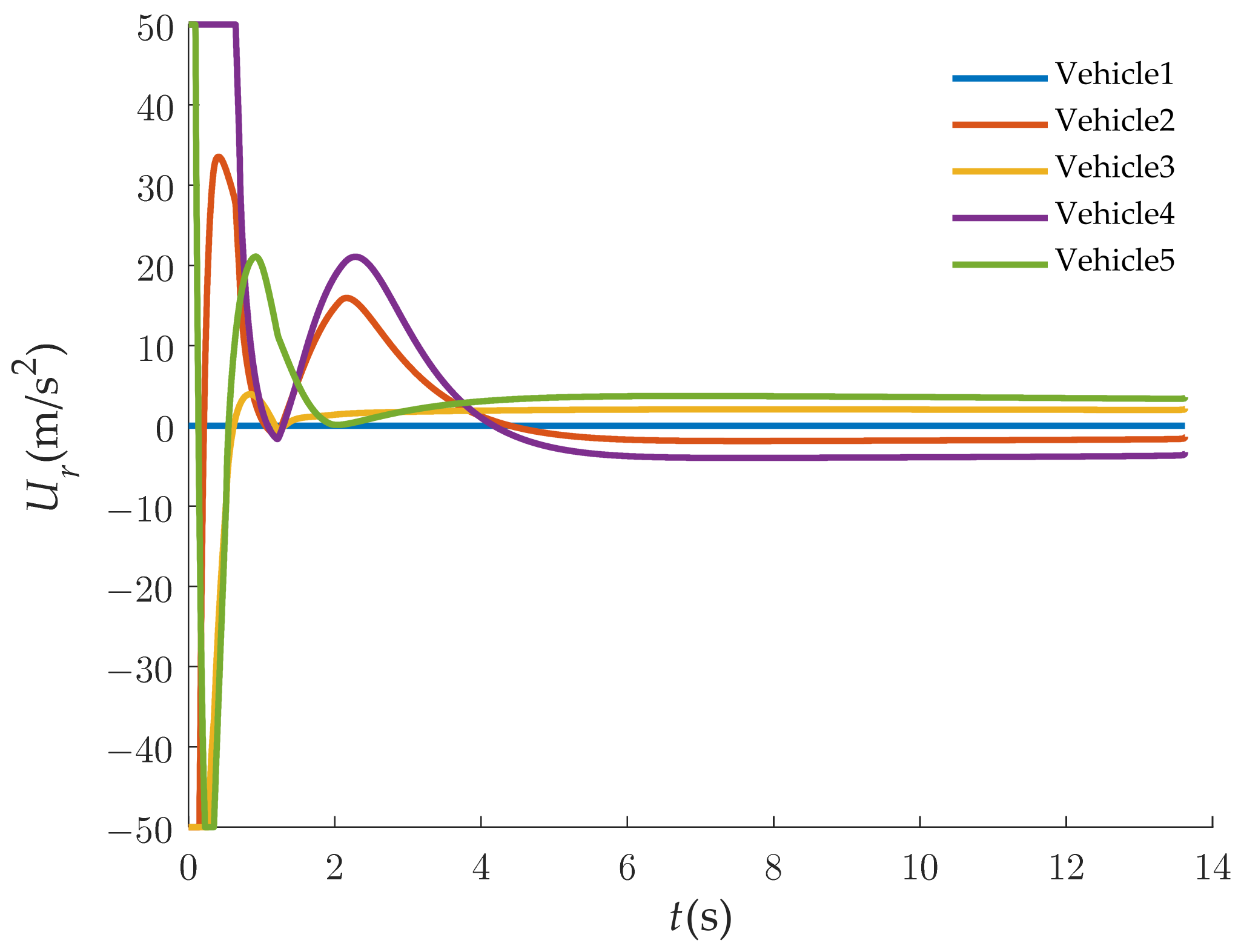
Figure 8.
Control commands in normal direction of LOS.

Figure 9.
Velocities of multiple vehicles.
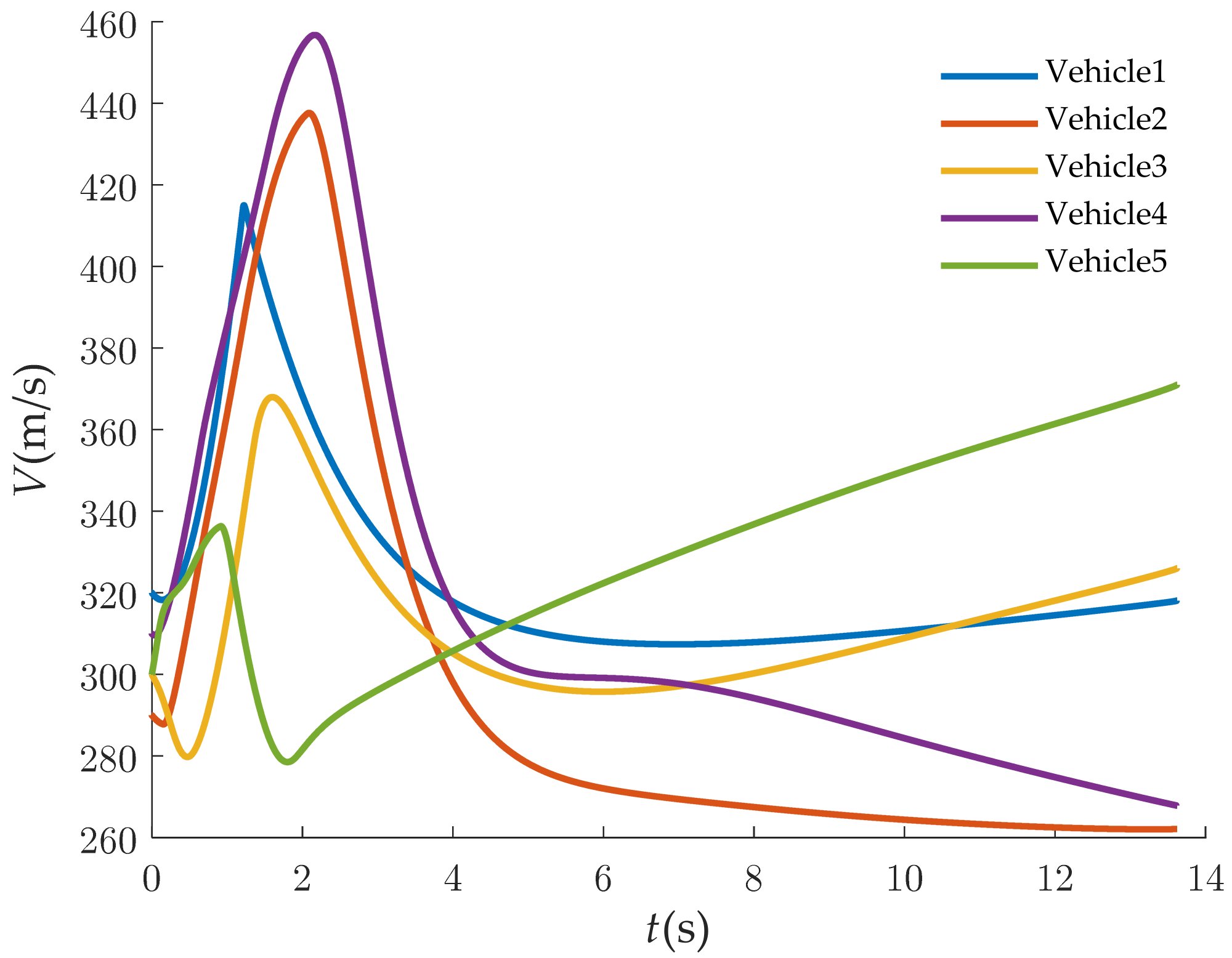
Figure 10.
Actual and estimated values of disturbance.
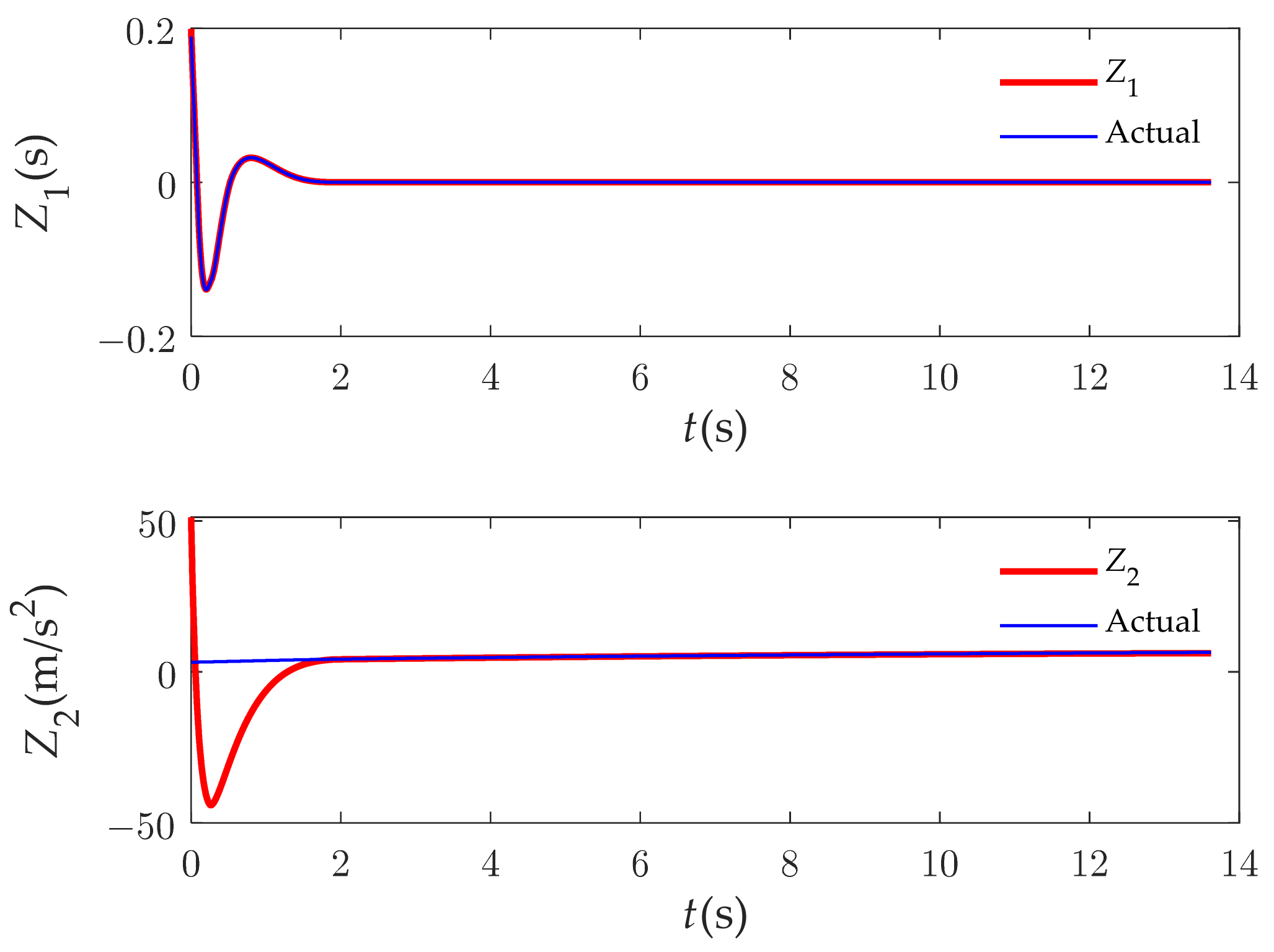
Figure 11.
Tracking error of DDOB.
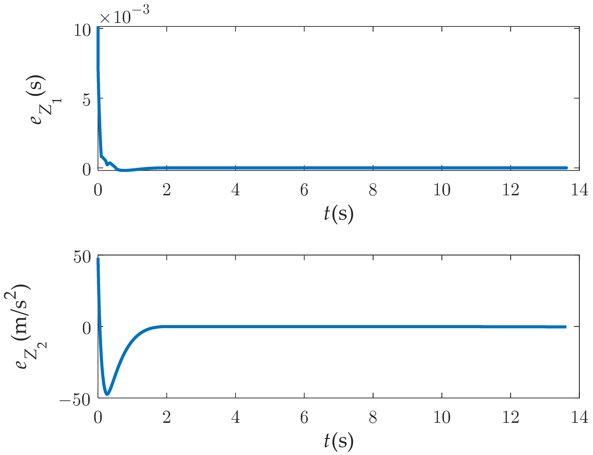
Figure 12.
Control-command comparison in LOS direction.
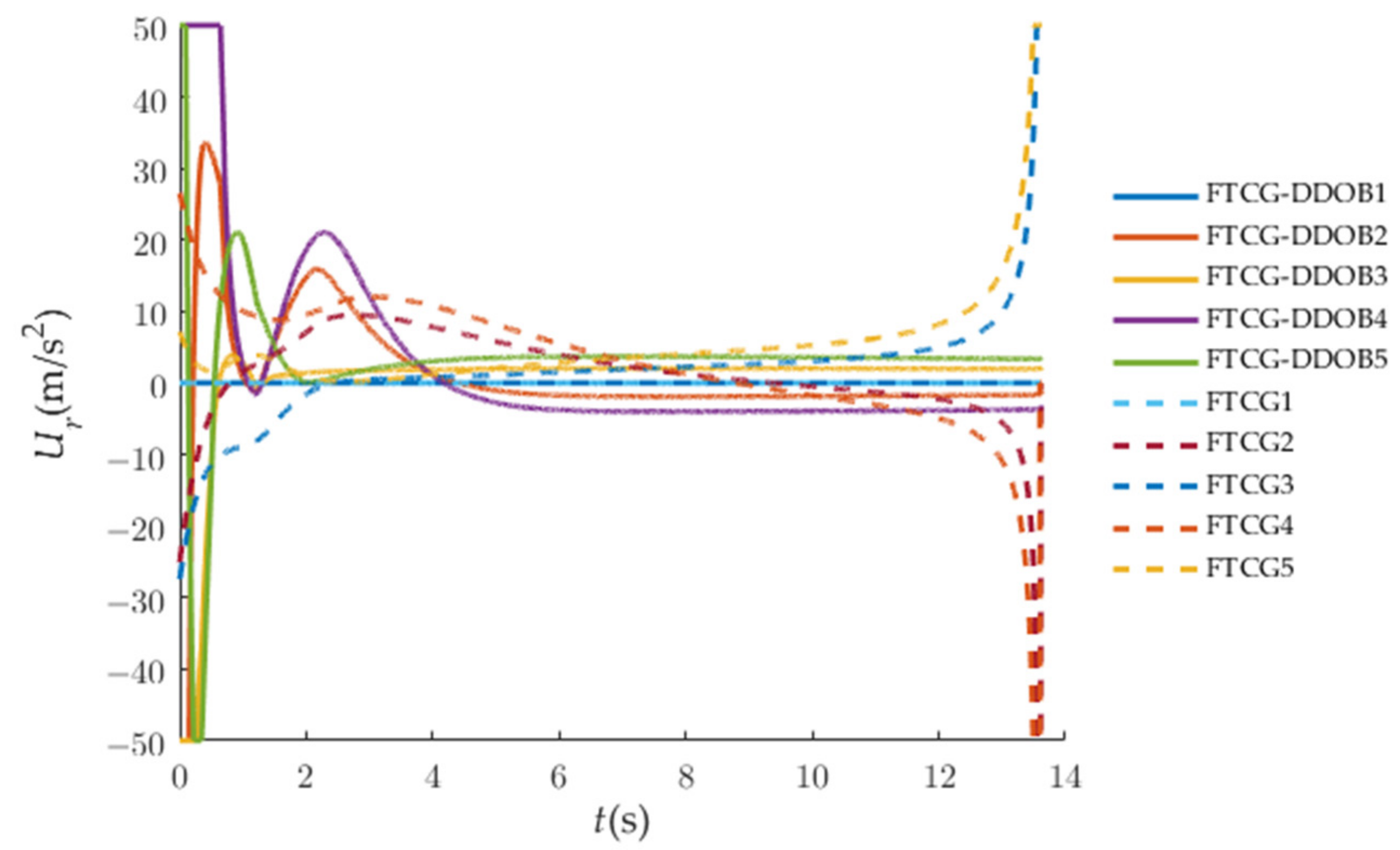
Figure 13.
Estimation-performance comparison between DDOB and ESO.

Figure 14.
Attack-angle comparison between PTCG and TSMG.
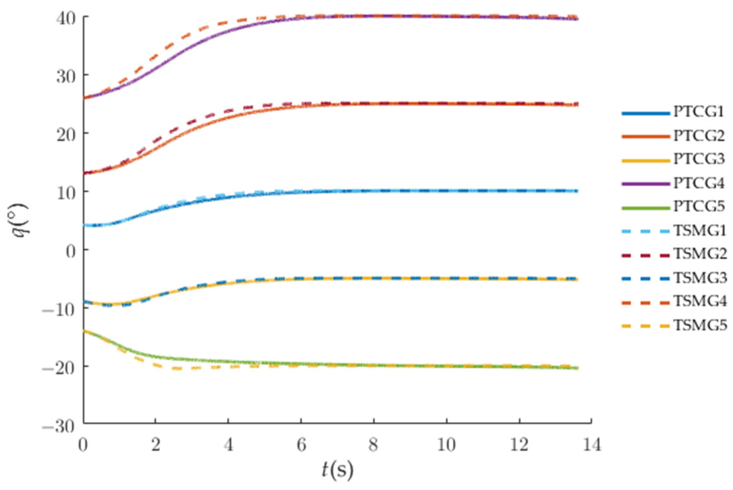
Figure 15.
Control-command comparison in normal direction of LOS.

Table 1.
The initial conditions of the interceptors.
| Vehicle | Initial Position (m, m) | Initial Heading Angle (°) | Initial Velocity (m/s) |
|---|---|---|---|
| M1 (leader) | (3000, 6500) | 10 | 320 |
| M2 | (3500, 5500) | 6 | 290 |
| M3 | (3700, 8000) | −5 | 300 |
| M4 | (3800, 4000) | 2 | 310 |
| M5 | (4000, 8500) | 5 | 300 |
Table 2.
The initial conditions of the target.
| Initial Position | Initial Heading Angle (°) | Initial Velocity (m/s) | Accelerated Velocity (m/s2) |
|---|---|---|---|
| (10,000, 7000) | −170 | 220 | 0.8 g cos(t) |
Publisher’s Note: MDPI stays neutral with regard to jurisdictional claims in published maps and institutional affiliations. |
© 2022 by the authors. Licensee MDPI, Basel, Switzerland. This article is an open access article distributed under the terms and conditions of the Creative Commons Attribution (CC BY) license (https://creativecommons.org/licenses/by/4.0/).
Share and Cite
MDPI and ACS Style
Guo, M.; Xia, G.; Yang, F.; Liu, C.; Liu, K.; Yang, J. Consensus Cooperative Encirclement Interception Guidance Law for Multiple Vehicles against Maneuvering Target. Appl. Sci. 2022, 12, 7307. https://doi.org/10.3390/app12147307
AMA Style
Guo M, Xia G, Yang F, Liu C, Liu K, Yang J. Consensus Cooperative Encirclement Interception Guidance Law for Multiple Vehicles against Maneuvering Target. Applied Sciences. 2022; 12(14):7307. https://doi.org/10.3390/app12147307
Chicago/Turabian StyleGuo, Mingkun, Guangqing Xia, Feng Yang, Cong Liu, Kai Liu, and Jingnan Yang. 2022. "Consensus Cooperative Encirclement Interception Guidance Law for Multiple Vehicles against Maneuvering Target" Applied Sciences 12, no. 14: 7307. https://doi.org/10.3390/app12147307
Note that from the first issue of 2016, this journal uses article numbers instead of page numbers. See further details here.