
Efficient Detection of Defective Parts with Acoustic Resonance Testing Using Synthetic Training Data


1
Fraunhofer Institute for Nondestructive Testing IZFP, Campus E3 1, 66123 Saarbrücken, Germany
2
Chair of Cognitive Sensor Systems, Saarland University, Campus E3 1, 66123 Saarbrücken, Germany
3
Chair for Lightweight Systems, Saarland University, Campus E3 1, 66123 Saarbrücken, Germany
*
Author to whom correspondence should be addressed.
Appl. Sci. 2022, 12(15), 7648; https://doi.org/10.3390/app12157648
Submission received: 17 May 2022
/
Revised: 14 July 2022
/
Accepted: 27 July 2022
/
Published: 29 July 2022
(This article belongs to the Collection Nondestructive Testing (NDT))
Abstract
:Featured Application
This study is useful for a series-integrated separation between good parts and defective ones via acoustic resonance testing. The work primarily relies on the simulation-based generation of mandatory and application-specific training data for defect detection. It also considers an optional use of additional structural component information in data evaluation. The given achievements may enable a time- and cost-optimized training procedure, allow for applying acoustic resonance testing despite a limited number of representative training parts, or provide a way to counter significant part-to-part variations for improved defect detection.
Abstract
Analyzing eigenfrequencies by acoustic resonance testing enables a fast screening of components regarding structural defects. The eigenfrequencies of each specific part depend on the general geometric and material properties, including tolerable part-to-part variations, as well as on possible structural flaws. Separating good parts from defective ones is not straightforward and each application-specific sorting algorithm is usually found from experimental training data. However, there are limitations and training data collection may be intricate. We worked on this challenge focusing on machine-made model parts varying slightly in geometry. The application objective was the eigenfrequency-based detection of parts featuring a through-hole test defect drilled into some of the parts and enlarged stepwise. The eigenfrequencies were measured concomitantly. Unlike the industry standard, our approach is based on synthetic training data created mainly by simulation techniques, which resulted in a principally satisfactory classification of the good and defective parts. However, the parts with small defects were not identified from the eigenfrequencies alone, due to overlaying geometric variations. In order to counteract such noise and to improve defect detection based on synthetic training data, the specific actual part geometry was used, in the sense of additional a priori information. A multimodal data evaluation model showed a clearly enhanced sorting power.
1. Introduction
A quality assessment of manufactured components can be achieved by evaluating the eigenfrequencies or other characteristics derived from the measured natural vibration behavior. Such an approach is referred to in relevant sources, among others, as acoustic resonance testing (ART) or resonance inspection [1,2,3,4,5,6,7]. Related to the research focus of this publication, ART aims at the series-integrated 100% quality screening of metallic or ceramic parts manufactured in large quantities and with short cycle times. The possible applications are manifold. They range from testing for cracks or other defects to analyses with regard to material mix-ups or microstructural anomalies. The particular advantages include the testability of an entire component volume in seconds, favorable hardware costs, excellent automation options, and environmental friendliness. Various implementation options are available for the respective ART steps, connected with specific advantages and challenges. However, an ART usually involves an active mechanical excitation of the test object (for example, impact or sweep excitation), followed by recording the vibration response (for example, via a microphone or with a contact sensor). After the signal acquisition and digitalization, various filtering and transformation steps as well as methods for the extraction of acoustic characteristics, such as eigenfrequencies, amplitudes, or damping values, may be carried out with the measurement data. By applying a suitable algorithm to the signal data or the derived acoustic characteristics, the test object is finally classified with regard to the application objective, for example, categorized as good or as defective.
ART is an acoustic method in the field of nondestructive testing (NDT). In contrast to ultrasonic testing, which focuses on the local interaction of sound waves with anomalies, ART analyzes the resonant vibration behavior of the entire test object. There are also other approaches that use such vibrations, for example, resonant ultrasound spectroscopy (RUS). RUS can be used for the nondestructive evaluation of the elastic properties from defined samples, based on a swept sine excitation. However, despite this common target of RUS including the evaluation of high frequencies and special algorithms, the term RUS is also used in NDT with regard to structural defects, see [6,7]. In this sense, RUS and ART, among other common names, are synonyms. For the purpose of a thematic delimitation, we limited the scope in the following to the works that are directly related to ART as a fast NDT-screening method for mostly engineering series parts that are subject to practice-effects.
Within the last ten years, some works focusing on the ART detection of cracked automotive parts were performed taking advantage of intelligent classification methods [8,9]. For the good defective distinction of tubular components, the ART data were evaluated in combination with the component weight and hardness [10]. ART was used for the characterization of ceramic tiles regarding the effects linked with the mechanical properties and processing parameters [11]. Other studies dealt with the evaluation of the natural vibration behavior of some samples produced by selective laser melting [12,13]. ART was also used for analyzing additive lattice structures [14,15]. Swept-sine excitation was used to examine additively manufactured bulk parts, based on their natural vibrations [16], or to evaluate aerospace components, with respect to their metallurgical properties and defects [17]. A further work addressed microstructural variations or anomalies within cast iron test samples with the help of ART [18]. There are other studies that focused on composite materials by analyzing the eigenfrequencies for damage detection [19,20]. Moreover, machine-learning algorithms were applied to ART data and used for the separation of healthy and damaged glass bottles [21], or for the classification of Euro coins [22]. There are also several studies dealing with ART-like approaches to various agricultural products, such as eggs or fruit [23,24,25].
ART is physically based on the free natural-vibration behavior of a body, which depends on its mass and stiffness distribution, or in engineering terms, on its geometry, the elastic constants of the material, and its density. In addition, the entire mechanical system, and thus the natural vibrations, are affected by various structural anomalies [26,27]. Consequently, the eigenfrequencies of a component reflect its general mechanical properties, but also its specific expression in terms of geometric and material part-to-part variations or possible macroscopic defects, such as cracks or voids. From measured eigenfrequencies, it is not straightforward to make conclusions about the structural condition of a part, because different effects cause individual spectral shifts superposing on each other. Therefore, a reliable quality statement with ART is anything but trivial and requires a suitable algorithm to solve the inverse problem. This arises especially where large tolerable part-to-part variations occur or small anomalies are to be detected. Some ART companies advertise statistical algorithms that should be able to detect parts with defects or structural anomalies by outlier detection, assuming predominantly healthy parts. However, most of the ART systems or applications rely on an explicit application-specific calibration or on a training procedure built on empirical data, respectively. A corresponding training dataset must be generated beforehand by measurements of many representative parts. Thereby, the anomalies to be detected, ideally covering all of the possible expressions, as well as tolerable part variations, must be included. This results in the need for expensive or complicated reference methods to achieve the quality states of the training parts. A large number of parts is required, which may not be feasible for defective components from a series production with low rejects. There are also disadvantages from a practical point of view. Since component modifications reflect in the natural vibrations, they may require an update of the training data collection. In addition, the application of ART to a new part type requires the training data generation initially, which makes it usually not possible to use ART synchronously with a production launch. In summary, experimental ART training data generation may be inflexible, difficult, extensive, time consuming, and cost intensive. This study addresses the challenges connected with the experimental procedure by a strategy that focusses on the simulation-based generation of synthetic ART training data for ART defect detection.
Although we found no work that is directly focused on the special topic of this study, other publications provided relevant findings. It is well known that the finite element method (FEM) can be utilized to simulate natural vibrations. The FEM data can be used, for example, for general purposes and for the evaluation versus measurements, or for sensitivity analyses with regard to geometry, material properties, or structural defects [8,13,27,28]. FEM simulations can quantitatively match the eigenfrequencies measured with ART very accurately, provided that the mechanical component properties are precisely known and modeled. Furthermore, the resonance spectra shifts caused by defects or due to other component variations were examined. Some approaches for the algorithmic separation between these different effects derived from the FEM data were published in literature [29,30]. Other papers focused on the eigenfrequency shifts calculated by extensive FEM studies related to the position of a small defect or stiffness change, respectively. Based on such FEM data, conclusions were drawn algorithmically about unknown defects from a given set of eigenfrequencies [31,32,33]. A simulation-based generation of synthetic ART training data was initially addressed in our previous publication, with an application focus not on defect detection, but on the correlation between the geometries and the eigenfrequencies of undamaged parts (some material, datasets, and essential facts are revisited here, without giving the reference designation each time again to avoid repeated citation) [34].
To summarize, the literature covers many ART application-oriented publications, but also addresses the challenges connected with an experimental generation of ART training data. The simulation techniques, such as FEM, were identified as sufficiently powerful to generate the eigenfrequency data, which can allow the development of various ART data evaluation strategies in general. Other aspects that are addressed, such as the need for a method to distinguish between the influences of defects from those of tolerable variations or the achievements towards an inverse defect detection considering various defect positions, are relevant points for this study. While existing works demonstrate the usefulness of simulated data for developing algorithmic approaches, there is no systematic approach to the application to sets of real parts. It is pointed out that further research is needed, for example, with respect to the effects such as random part variations, the offset of the simulation data to the measurement data, or other practice-relevant effects. In contrast, the strategy, which will be presented, covers all, undamaged and defective parts, tolerable part-to-part variations, and the fundamental deviations of the simulation data from measurements. Moreover, the procedure is not only described in detail or discussed theoretically. It is also verified during a fictitious application scenario, by means of machine-made model parts and ART measurement data.
Figure 1 outlines our strategy for setting up any specific ART application (for defect detection) based on synthetic ART training data. The essential steps are:
- Step no. 1 is the generation of the simulation data representing the part type, possible defect type(s) of interest, or the magnitude and nature of the tolerable part-to-part variations in a realistic manner. This entails actual simulations, as well as data enhancement or scaling methods. Furthermore, an adaption of the simulated data to corresponding measurement data is needed to reduce any systematic deviation of the synthetic data versus the measurement data. This can be achieved from a few machine-made reference parts that are characterized experimentally and are then rebuilt in the virtual world;
- Step no. 2 consists of finding a suitable ART sorting algorithm from the synthetic training data set. The sorting algorithm depends heavily on the target of an ART application, which here is defect detection. However, it does not need to be different from the procedure in the case of experimental training data;
- Step no. 3 covers the validation of the simulation-based ART training procedure via machine-made parts or the series application of the found ART sorting algorithm.
Section 2 of this publication contains a description of the part type considered for the application scenario, including geometric part-to-part variations. The possible defect is introduced with regard to type, size, and position. In addition, the background and the settings used for the FEM simulations are presented. This includes a snapshot of the natural vibration behavior of the part type and an analysis of the defect impact on the eigenfrequencies versus the frequency shifts caused by geometric variations. The theoretical limits of a simple defect detection approach using one single eigenfrequency are shown. Afterwards, some machine-made parts are introduced. The experimental methods that were used for the data acquisition are described. The application scenario and further assumptions for a practicable classification algorithm are addressed. Section 3 deals with the realization of our approach, including all of the steps as summarized in Figure 1. This means that the specific generation of the synthetic ART training data is described first. Next, several classification models or sorting algorithms are introduced, including the background of their design. This also includes a theoretical validation process. Finally, the results from the application of the derived defect detection models towards more than twenty machine-made parts are presented. Since the addressed application scenario uses measurement data, but is still fictive, Section 4 contains a discussion with a focus on a practical series-integrated ART defect detection, based on synthetic training data. Future research tasks for ART are also discussed. Section 5 summarizes the essential aspects of this work.
2. Materials and Methods
2.1. Part Type and Random Geometric Part-to-Part Variations
Connecting rods were selected as the exemplary parts. Figure 2 visualizes the geometry of this model-like part type. Since each part is symmetrical with respect to the x–y-plane and the x–z-plane, the geometry can essentially be quantified with eight geometric parameters. The parameters dR1 and dR2 or DR1 and DR2 describe the inner or the outer diameters of the rotationally symmetrical cylinder rings, respectively. The two cylinder ring heights are identical and indicated with hR. The bar area has a cuboidal shape with the width wB and the height hB. The bar length is set via lR, which is the distance between the cylinder ring axes. There are additional edge fillets with a constant radius of 3 mm.
Random part-to-part variations in geometry are relevant when using ART. To describe such variations, normal distribution was chosen. Each of the eight geometric parameters was connected with a stochastically independent normally distributed random variable, which itself is quantified by a mean value and a standard deviation. The defined mean values and standard deviations are also shown in Figure 2. We use the term basic population in this manuscript to indicate a random population of connecting rods, whose geometry varies normally distributed with respect to the values given in Figure 2.
Approximately 99.73%, and thus almost all of the possible values, of a normally distributed random variable deviate no more than three standard deviations from the mean value. Having regard to this, the essential geometric ranges of the basic population are covered by the accuracy class c (coarse) or at least v (very coarse) of the general tolerances, according to DIN ISO 2768, see [35]. This means that such variations are large, but still realistic, especially for unfinished blanks produced with a forging or casting process.
Besides the basic population, some populations with other probability distributions (scaled normal distributions, uniform distributions) were defined. All of the random parts, either virtual parts that only exist as computer models or machine-made parts that are produced according to given nominal dimensions, were specified with independent random numbers. These numbers were created with the MATLAB® functions normrnd (normal distribution) and unifrnd (uniform distribution). Often, the same sets of random numbers were used multiple times, for example, to achieve batches of parts with identical geometries, but different defect specifications. This was realized by controlling the random number generator via the function rng, in combination with specific seed values.
In addition to the parts with random dimensions, a geometrically non-random connecting rod, called geometrically mean part, was defined as a reference. The geometric dimensions of this part are the mean values shown in Figure 2.
The connecting rod material was chosen to be homogeneous and constant with isotropic elastic properties, as far as technically possible for the machine-made parts.
2.2. Defect Type to Detect
Each connecting rod can feature an optional defect, which means that there is a single defect, or that the part is defect-free. A cylindrical through-hole with an alignment of its axis in the z-direction was chosen as the defect type. This defect type was chosen for the fictitious application example, due to its good implementability in simulation models as well as in machine-made parts by drilling. The defect diameter of interest is in the range from 1 mm to 3 mm with an even probability of occurrence. Figure 3 shows the possible defect positioning. A defect occurs either within one of the two cylinder rings, exactly placed between the inner and outer cylinder ring wall (it is centered on one of the red circles in the sketch, but any position on the circles is possible). Alternatively, a defect is located in the bar area, with the defect axis being at least 4 mm away from the bar edges and the cylinder rings (it is anywhere inside the red shaded area, or it is even centered on the red lines in the sketch). The defect position limits were chosen to avoid breakouts towards the edges and to ensure that a reasonable residual wall thickness always remains, independent of the geometric dimensions, defect position, and defect size. We assume the defect position to be random within the given explanations. This means that the three defect domains are considered with the same probabilities and no subdomain is more likely than another subdomain. However, for general investigations or for ART training data generation, for example, more extreme defect sizes or special defect positions were examined.
2.3. FEM-Simulated Natural Vibrations and Basic Data Insights
2.3.1. FEM Simulations and Eigenmodes of a Connecting Rod
To access the eigenfrequencies and eigenmodes of the virtual connecting rods, FEM simulations were performed using COMSOL Multiphysics® (basic software plus Structural Mechanics Module, version 5.2a). Perfect linearity was supposed and quadratic 3D tetrahedral elements were used. As the maximum element size, 1.1 mm was chosen. Additionally, damping was ignored during the simulations and each object was set to be free without any external support or fixation. For all of the simulations, a homogeneous material, with a density of 2700 kg/m3 and an isotropic elasticity, was assumed (Young’s modulus: 70 GPa; Poisson ratio: 0.34; shear modulus: 26.12 GPa). These values are typical for an aluminum alloy. They were selected with regard to the machine-made parts described later.
Figure 4 shows the FEM-calculated eigenmodes assuming the geometrically mean part. There are 18 eigenmodes up to a frequency of 30 kHz, which have either bending, torsional, or longitudinal character. The eigenmodes are named as Mode-1, Mode-2, …, Mode-18, according to the ascending eigenfrequency order observed for the geometrically mean part. The eigenfrequencies vary in a mode-specific way as a function of the specific mechanical part structure. The eigenmodes stay the same for the different parts with individual geometric dimensions in a qualitative manner, however, they can occur in another order compared to the geometrically mean part. We always used the eigenfrequencies sorted by identified modes (and not by ascending frequency values) for this study.
2.3.2. Geometry-Induced Eigenfrequency Shifts versus Defect Impacts
Understanding the relationship of the specific structure of a part towards its eigenfrequencies is fundamental for reaching a reliable defect detection. Based on FEM, Table 1 gives an estimation of the connecting rod eigenfrequencies depending on the geometric effects, together with an optional through-hole defect of 2 mm diameter in the center of the bar (central 2 mm defect). Besides the geometrically mean part, different batches each containing 1000 virtual parts from the basic population with or without defect were used to generate the table data. Table 1 contains the following mode-specific information:
- Frequency without defect: This column contains the eigenfrequencies of the geometrically mean part without any defect. The averaged frequencies of the defect-free parts derived from the basic population are roughly the same;
- Geometry-induced standard deviation: These columns contain the standard deviations of the eigenfrequencies that can be obtained for the normally distributed basic population (the frequencies are also nearly normally distributed). The values refer to the defect-free parts, but approx. identical standard deviations can be observed for the parts with a central 2 mm defect. The values are given in absolute and relative terms;
- Frequency shift due to a central 2 mm defect: These columns present the eigenfrequency shifts or defect impacts induced by a central 2 mm defect. The shifts refer to the geometrically mean part. On average, similar shifts can be observed for the defective parts from the basic population, all featuring an identical, central 2 mm defect. However, the individual defects’ impacts depend significantly on the specific random part geometry. The values are given in an absolute and relative manner.
Referring to the geometrically mean part, the defect impact with respect to the defect position and size was analyzed with FEM. Figure 5 visualizes the impact of a 2 mm defect at various positions in the bar for some eigenmodes. Such nonlinear and mode-specific behavior depending on the defect position is well known [29,36]. However, a useful defect detection requires the consideration that a defect can influence an eigenfrequency with an individual maximum or has nearly no effect, which strongly depends on the defect position.
Since a linear growth in the defect diameter results in a quadratic rise in the defect area and volume, a quadratic dependence of the defect-induced frequency shift from the defect diameter was expected. Once again, using the fixed defect position in the center of the bar, such behavior could approximately be confirmed for the moderate defect sizes up to 3 mm or 4 mm, which is sufficient for our range of interest. Nevertheless, there are more complicated or interactional effects in the case of a larger defect, or in the case of a variable defect position in combination with geometric variations. For example, a large defect has an impact on the geometry-induced eigenfrequency standard deviations of a population, even if the position is fixed. Of course, when the defect position is also variable, this has an additional impact on the statistical characteristics. The nonlinear frequency shifts caused by a defect in a random position combined with an individual part geometry can then cause very individual eigenfrequency shifts versus the geometrically mean part.
2.3.3. Theoretical Limits of a Simple Eigenfrequency Defect Detection
One single eigenfrequency is generally not suitable for an ART defect detection, because a frequency may not be significantly affected or sensitive to a defect, depending on its position. Therefore, an approach based on a single frequency can only work for special defect positions. In addition, the defect influence may be much less compared to the geometry-induced effects on the eigenfrequencies. Therefore, geometric scatter can superpose the effects from the structural defects. FEM data were used for an estimation of the defect detection limits for the connecting rods using a single eigenfrequency. A central through-hole defect in the middle of the bar was assumed as an example. Figure 6 is derived from Table 1. It refers to the parts from the basic population and visualizes the relative sensitivity of the connecting rod eigenfrequencies to a 2 mm defect. Every sensitivity value is the mode-specific ratio between the frequency shift caused by the defect on average compared to the eigenfrequency standard deviation caused by the geometric variations. As can be seen, Mode-16 has the highest sensitivity towards such a central 2 mm defect.
Figure 7 visualizes the distribution of the eigenfrequencies regarding Mode-16 for large batches of defect-free parts and for parts with a central through-hole. The figure shows density curves derived for the basic population parts, as well as for the parts from a scaled population with only 10% geometric scatter in cross-comparison. There are curves for the different defect sizes. In the case of the basic population, there is no chance of a reliable separation between the damaged parts containing a defect with a diameter from 1 mm to 5 mm and the good parts, due to a significant overlap of the frequency ranges. A separation may only be possible for large defects with a size of 10 mm or more. This, however, is an academic finding and not a demonstration of a satisfactory performance. In contrast, for the small geometric variations, the defects with a size of around 3 mm or larger should, in theory, be detectable with the help of that single eigenfrequency. Nevertheless, the utility for a defect detection is still limited to special positions and a 3 mm defect is quite large, taking into account the low geometric variations. Furthermore, these results are based on simulation data and practice-relevant effects may result in a reduced detection power.
The previous explanations illustrate that a simple ART defect detection approach based on a single eigenfrequency is extremely limited. This is particularly valid in the case of large variations in the geometry from part to part or when a possible defect is not limited to a small and known region of a part. To counteract the observed challenges, we describe a much more powerful approach within this paper, based on a more efficient data evaluation method as well as on extensive synthetic ART training data.
2.4. Machine-Made Parts and Experimental Data Acquisition
A set of 29 machine-made connecting rods manufactured in a workshop was characterized experimentally. Five reference parts were used, which are indicated with the letters A to E. These parts were machine-made, following the geometrically mean part, which means that the identical mean geometry was set as the nominal geometry. Additionally, two dozen validation parts were used. These parts were labeled with consecutive numbers from 1 to 24. The nominal geometric dimensions of the validation parts were set with random numbers, considering the basic population and its value ranges. For the parts no. 1 to 12, the normally distributed basic population was imputed directly. For the parts no. 13 to 24, a uniform distribution was selected instead, whereby the interval borders are the mean value plus or minus three times the standard deviation of the basic population for each geometric parameter. Due to the limited amount of machine-made parts, the uniform distribution was chosen to describe many parts that are more likely to have values near the borders of the essential value ranges instead of being more centered with a higher probability. However, the part geometries could also come from the basic population, because all of the dimensions are inside the typical value ranges of the basic population. For some parts, a single dimension was manually set to the mean value plus or minus four times the standard deviation. This should achieve dimensions slightly outside the usual ranges. It is noted that all of the nominal geometric values were rounded to integer multiples of 0.05 mm for better handling. Finally, the parts were machined from a single batch of rolled aluminum alloy, according to the defined geometric dimensions. Using a single material batch should ensure a nearly constant material behavior. Additionally, a consistent production strategy was agreed with the manufacturer to reflect a reproducible series process.
Through-holes representing structural defects were drilled into 14 of the 24 parts, using a conventional pillar-drilling machine and enlarged stepwise. We selected the parts no. 1 to 7 and no. 13 to 19 for the defect implementation. The process started with a defect diameter of 1 mm and resulted in a final size of 3 mm, with steps of 0.5 mm. The defect position was individual for each part. The defects were placed manually over the parts to achieve a uniform defect distribution, considering the limited number of parts and taking into account that the application example does not assume any preferred defect positions. Symmetry was taken into account to avoid similar positions due to the limited amount of parts. Figure 8 shows the chosen defect position depending on the part number. The actual positions can vary up to 1 mm in the lateral directions compared to the sketch, because the positioning was completed by hand and not by machine. In addition, the figure includes photos of two of the machine-made parts with their final 3 mm defect size.
The machine-made parts were characterized experimentally as briefly described in our previous publication. For example, we recognized a homogenous but slightly anisotropic material behavior linked with the rolling structure of the material and discovered, with the help of radiography, that the parts featured no macroscopic volume defects. During the measurements, the temperature was measured and the temperature effects on the quantitative measurement data were computationally corrected to the best possible accuracy.
Before implementing the through-holes, all of the connecting rods were measured geometrically, because each actual geometry differs inevitably from the nominal dimensions due to production tolerances. A coordinate measuring machine was used for this. The measured data were then applied to our geometry model. This means that the dimensions regarding the eight geometric parameters were updated, although the measuring machine provided additional information, such as small deviations from perfect symmetry. The updated geometry data included averaged cylinder ring heights, since the initial results contained individual heights for both of the cylinder rings indicating some offset. However, all of the observed uncertainties towards the idealized geometry were small and not critical.
The eigenfrequencies of the parts were measured with ART. This was initially completed before drilling the through-holes into some of the parts. After each step of defect enlarging, the ART measurements were repeated to record the eigenfrequencies depending on the defect size. For the ART measurements, the part to be examined was placed on three rubber tips. A manual impulse hammer was used for excitation and a microphone recorded the sound signals. Several excitations at different points were carried out on each part to ensure a stimulation of all of the relevant eigenmodes. To minimize the effect of random fluctuations or outliers, each part was measured at least five times in each defect condition. Single outliers were identified and eliminated. The frequencies were finally averaged, resulting in 18 experimental eigenfrequencies per part and per defect condition.
In addition, we performed associated FEM simulations of the defect-free states, as well as considering the different defect sizes. These simulations were carried out using the metrologically updated geometries. On the one hand, the simulated eigenfrequencies were used to match and sort the measured eigenfrequencies to the eigenmode numbers (a laser Doppler vibrometer measurement and amplitudes from the ART data, depending on the direction of excitation, delivered further information for this purpose). On the other hand, the simulation data served to access the systematic deviations between the simulated and measured eigenfrequencies, which is central for this work.
2.5. Overview and Further Specifications for the Application Scenario
The application scenario is focused on the detection of defective connecting rods via ART, under the additional boundary condition that the parts also vary randomly in their geometric dimensions. As the defect to detect, a through-hole with a size between 1 mm and 3 mm was chosen, whereby a part features exactly one single through-hole or none. Multiple holes or other defect types were not allowed. Material variations were avoided as far as possible. A set of 18 eigenfrequencies, being used as the mandatory classification input, and either four or all of the eight geometric dimensions per part, being used as an optional input, formed the basis for each test decision with respect to a defect. To design the application scenario unambiguously and to achieve an appropriate optimization of the classification problem, the scoring of any misclassification, as well as the probabilities of occurrence for the undamaged and defective parts, also had to be taken into account.
Within a real series production, whether a defective part is overlooked or a good part is mistakenly rejected will usually have different degrees of severity. This can have safety-critical or economic reasons. Our application scenario is fictive and only serves for demonstration. Therefore, we did not specify any additional constraints and remained neutral with regard to the scoring of misclassifications. Any mixing up of the good parts with the defective parts or vice versa by a classification model was seen critically in the same way during the data evaluation. Furthermore, good parts are usually more frequent in a series production. Some of the possible defect types, positions or sizes can also be more likely than others. However, defining specific constraints would have been speculative, especially because finding an allover optimizing classification rule can highly depend on the assumed probabilities of occurrence. Therefore, we once again remained neutral to ensure a balanced quality evaluation. This means that we assumed that the good parts and defective parts would occur with an equal fifty-fifty chance. In the case of damage, each of the defined defect domains should occur with a probability of 1/3. Additionally, within each of these domains, the defect specifications are random and uniformly distributed, with no subdomain being more likely.
In the end, the application scenario aims at the discrimination of the good parts and the defective ones. For the classification models with multiple defect classes, the assigned defect size or defect position of a classified part was only considered secondarily. Rather, it was primarily evaluated whether a part had been correctly or incorrectly assigned to the good class, or to any defect class at all. In other words, the decisions were mostly retrospectively reduced to a two-class system (good/defective) and then evaluated. The evaluation was completed with the help of TPR (true positive rate) and TNR (true negative rate) [37]. These metrics represent the proportion of the defective parts that are also classified as damaged (TPR) or the proportion of good parts that are also classified as (TNR).
3. Results
3.1. Simulation-Based ART Training Data Generation
The first step of our application scenario demonstration covered the generation of the ART training data based on simulation techniques (see Figure 1). The training data generation included FEM simulations of connecting rods, but also further partial steps that aimed to enhance the amount of simulation data and to adapt it to measurement data.
The geometric dimensions of 5000 virtual training parts were described with random numbers. Contrary to the basic population, uniform distribution was chosen for the virtual training parts. This ensured that no subrange of the training data was more common. The uniform distribution interval borders were set to the mean values plus or minus 4.5 times the standard deviations of the basic population. Since the essential values of the basic population differed by a maximum of three standard deviations from the respective mean values, by 50% increased ranges were assigned for the virtual training parts. This scaling ensured that the training data confidently covered the geometries of the machine-made parts (or of any of the basic population parts subjected to a defect detection).
The structure-dependent eigenfrequencies of the virtual training parts with respect to Mode-1 to Mode-18 were calculated by FEM. The simulations were initially performed without any defect. Afterwards, the simulations were repeated three times, assuming again 5000 virtual parts each time with the same individual geometric dimensions as before, but considering a through-hole defect either in one of the two cylinder rings or in the bar area. This entire set featured defective parts with a 2 mm through-hole appearing uniformly, and randomly distributed within the defined defect domains. As an output, we obtained the geometric data and eigenfrequencies of 5000 defect-free virtual trainings parts and the corresponding data for the geometrically same parts, but with a randomly positioned 2 mm defect within one of the cylinder rings or the bar area.
To achieve a suitable ART defect detection, the training data generation had to take into account that the eigenfrequencies of a defective part depend, in a nearly quadratic manner, on the defect diameter. However, performing further FEM simulations assuming many other defect sizes would have resulted in a large computational effort. To counteract this and to enhance the data effectively, we took advantage of the recognized defect size behavior and the fact that the geometric dimensions of the defect-free training parts were used again for the FEM simulations including a 2 mm defect. The eigenfrequency deviations from the defective to the good parts were calculated. These deviations can be seen as the isolated impacts of a randomly positioned 2 mm defect in each case. We scaled these defect impacts by using the quadratic dependence from the defect diameter. For example, a 1 mm defect causes approx. one quarter of the impact of a 2 mm defect at the same position. In this way, the defect impacts from 0.8 mm to 3.6 mm with an increment of 0.1 mm were derived (since the aim is the detection of any defects from 1 mm to 3 mm in size, 20% smaller or larger values were chosen). Finally, the impacts of the scaled defects were added to the eigenfrequencies of the 5000 defect-free parts for each defect size, resulting in a much more extensive data set. If we had generated all of the data directly with FEM and not enhanced them, we would have had to perform 440,000 calculations instead of 20,000 FEM calculations (5000 good parts + 3 × 5000 defective parts × 29 defect sizes).
Since the simulation-based data differed from the measured data due to many simplifications or inaccurate assumptions, as discussed extensively within our previous publication, the synthetic data set had to be adapted to the measurement data. The five machine-made reference parts were taken into account for this. Their associated FEM-calculated eigenfrequencies were evaluated versus the frequencies that were measured by ART. A similar offset behavior between the simulations and the measurements was found for all of the parts, which clearly depends on the eigenmode. This indicates that an easy multiplicative adaption via mode-specific correction factors is suitable. Table 2 shows the correction factors (measured data divided by simulated data), which were averaged from the reference parts depending on the eigenmode and finally applied to the synthetic training data.
Although the five reference parts show similar deviations between the simulation and the measurement data, the deviations are not exactly the same. For analyzing the quality of the correction factor method, one reference part was excluded and the correction factors were averaged again from the remaining parts. Then, the factors were applied to the simulated eigenfrequencies of the excluded part. Finally, the adapted simulation data of the excluded part were evaluated again versus its measured frequencies, which led to small residuals. Figure 9 shows this for the five reference parts, which are indicated with the letters A to E. The data transformation from the simulation to the measurement world is not perfect, but the remaining differences of the adapted simulation data to the measured values are, in nearly all of the cases, in terms of amounts smaller than 0.1%, indicating a good performance of the correction factor method.
To cover an imperfect data adaption by the correcting factors, three scenarios for the synthetic ART training data were subsequently considered. The synthetic training data were used directly for the ART training procedure. Additionally, uniformly distributed random noise was applied to each frequency value of the synthetic training data, either in the relative range from −0.1% to +0.1%, or from −0.3% to +0.3%, respectively. This was executed to represent the uncertainty of the simulation data adaptation to the measurement world, in an order of magnitude as it was observed or in an exaggerated way.
3.2. ART Sorting Algorithm
The second step of our application scenario demonstration was the development of a suitable ART sorting algorithm for defect detection (see Figure 1). This was carried out on the synthetic ART training data, the generation of which was explained before.
For the classification task in this work, the specific model type or the selection of the most powerful algorithm was not the focus. The model type itself was seen more as a required tool for the demonstration and any suitable type satisfied our needs. Common classification types were examined. The MATLAB® function fitcdiscr (fit discriminant analysis classifier) was found to create suitable classification models, based on quadratic discriminant analysis classification (name-value argument for model type: ‘DiscrimType’, ‘pseudoquadratic’). We created different classification models, using synthetic ART training data either with or without additional noise, as well as with different sets of predictor variables. All of the models were designed incorporating the remarks from Section 2.5. Prior values were applied, which indicate a fifty-fifty chance for a part to be good or to be defective with a completely even defect distribution. A cost matrix, which controlled each of the training procedures through the assignment of cost values aiming at a low sum of cost, was defined as follows: 0 cost score for the correct good/defect classification; 1 cost score for confusing the good parts with defective ones or vice versa; 0.01 cost score for mixing-up the different defect classes.
Although the application scenario aimed to differentiate between the good and defective parts and not between the different defect sizes or positions, each virtual part or data row within the training data was labeled according to a multiple class-system, covering one good class and many defect classes. This was chosen to ensure a solid classification functionality, after understanding the heterogeneous effects of the defect size or its position to the eigenfrequencies of a part. This led to the knowledge that the defective parts do not form a single well-defined class that unambiguously differs from the good class. To put it clearly, defining the multiple defect classes should ensure that each class contains parts that have the most homogenous defect impact characteristics. The various defect sizes of the defective trainings parts were directly used for the labeling. Then, the labels were extended with information about the part subdomain in which the defect was located. Figure 10 visualizes the defined defect subdomains while taking into account the part symmetry. Both of the cylinder rings were divided into six subdomains each, with the bar area consisting of seven subdomains. Bringing all of the combinations of the defect sizes and subdomains together, the final class system covers a total of 552 classes (1 good class + 551 defect classes, with 29 defect sizes and 19 subdomains). We assumed that more classes may allow clearer results. However, the amount of classes was limited by two factors. First, an increasing computing power requirement was recognized, as more classes were used. Second, the classification can abruptly become very bad, which is likely due to the fact that there were too few training parts in each class to properly predict a large amount of the classification model coefficients.
The input or predictor variables used for the classification models comprised the available 18 eigenfrequencies of each part, as well as the geometric data as an optional input. When implementing the geometry, either the full eight geometric parameters were used, or only half of them (the inner cylinder ring diameters dR1 and dR2, the bar width wB, and the bar height hB). The square roots from all of the possible pairwise product terms regarding the geometry were calculated as further optional input terms of some of the models, resulting in a maximum of 28 (full geometry) or six (half geometry) optional predictor variables. Other terms were not taken into account, because this could have led to poor classification results due to too many inputs, which would have required even more training data than actually available, as a countermeasure. In addition, higher polynomial terms may have resulted in an over-fitted model that was no longer suitable for the application to the noisy measurement data. Since using the eigenfrequency interactions would have resulted in too many predictor variables (actually 153 interaction terms) for a sufficient model prediction, we did not consider them. For the distinct description of the classification models depending on the predictor variable configurations, we introduced short model identifiers. The letters F, G, and g indicate if the eigenfrequencies, the full geometry, or only half of the geometric information were considered for a model, respectively. Additionally, the numbers 1 or 2 show if the geometry data were only used directly (1) or if additional interactional terms occurred (2). For example, F describes that the eigenfrequencies alone were implemented, and F-G2 denotes a model that is based on the eigenfrequencies, plus the full geometric data including interactions.
Before applying the final classification models to the machine-made validation parts, the theoretical classification limits were analyzed with the help of new virtual parts or synthetic validation data. These synthetic data comprise 1000 defect-free parts from the basic population. In addition, many defective parts with the same geometric dimensions, but having a through-hole of 1 mm, 1.5 mm, 2 mm, 2.5 mm, or 3 mm either in one of the cylinder rings or in the bar area, were considered. Altogether, three times 1000 parts per defect size were fully simulated and not enhanced as within the training data generation to reach the most realistic defect behavior. The correction factors were applied to the simulated eigenfrequencies. This fitting to the measurement data allowed the synthetic validation data to be put directly into the calculated classification models, instead of recalculating the models. Figure 11 shows the results for the classification models F and F-G2, both derived with the help of the synthetic ART training data without additional random noise.
Each diagram in Figure 11 visualizes the classification results of the 1000 virtual parts and each single data point represents one part. The title indicates the classification model used, as well as the true quality state of the parts. The x-axis specifies the defect size that is connected with the predicted defect class, whereby the parts classified as good were plotted at a defect size 0 mm. The y-axis indicates the mean geometric deviation, which is calculated by averaging the absolute percentage deviations of the measured geometric dimensions in relation to the geometrically mean part. This metric, among others, was originally selected to evaluate if the classification results depend on the magnitude of the geometric scatter. We did not find such a relationship, but kept the metric for visual reasons. The model using additional geometric input data classified all of the parts accurately. The other model made several misclassifications of the defective parts with a through-hole in any cylinder ring. Furthermore, the more complicated model always roughly classified the defective parts with regard to the correct defect size, but the simpler model led to more classification scatter. In the end, Figure 11 illustrates a significantly better classification power of model F-G2 versus model F. However, this is only a small snapshot of all of the results.
Figure 12 summarizes the results that were achieved with the different classification models, based on the synthetic training data with different noise levels. The obtained TNR (true negative rate) and TPR (true positive rate) values, which indicate the amount of correct classifications for the good parts and for the defective ones, vary slightly with the random number sequences used for the geometric definitions and for applying noise. The TPR values were averaged over the three times 1000 virtual parts with a through-hole each.
From Figure 12, it can be seen that the good parts were classified correctly in all of the considered cases. In contrast, the classification results for the defective parts depend strongly on the classification model configuration and on the noise level of the synthetic training data. The additional use of the geometric data as linear or even interactional model input significantly improved the detectability of the smaller defects, but the defect detection became worse the more noise that was applied to the training data. Depending on this, an acceptable defect detection with a detection rate of at least 95% is given for defects of 1 mm or smaller, or only for defects significantly above 3 mm size. For the training data set with the medium noise level, the theoretical defect detection limit is between 1.5 mm and 3 mm, depending on the applied model configuration. Although improved modeling, such as including higher polynomial eigenfrequency terms, implementing more frequencies, or even using other classification types, may slightly improve the defect detection, there may be a limit when using the eigenfrequencies alone. This is because the spectral shifts are not only an indication of a defect, but they are also caused by tolerable structure configurations. This makes it challenging from a certain point to find a clear quality conclusion from a given set of eigenfrequencies without any further component information. Nevertheless, the results achieved on the virtual parts indicate a good chance of separating the defective machine-made parts from the good ones, at least above a certain defect size.
3.3. Validation on Machine-Made Parts
The third step of our application scenario demonstration covers the validation of the derived ART sorting algorithms for defect detection (see Figure 1). This is pointed out on the two dozen machine-made validation parts and their measurement data.
Before applying the final classification models to the machine-made parts, we derived some illustrative visualizations for the separation task between the good parts and the damaged ones. The related idea is to predict the eigenfrequencies of a part from the individual component structure data being variable within a population from part to part, meaning from the full geometric information in the case examined here. The deviations between the predicted and the actual eigenfrequencies of an undamaged part should be close to zero, provided that the frequency predictions are reliable. In contrast, large deviations in the frequencies can indicate that the actual eigenfrequencies of a part are affected by a structural impact, such as a macroscopic defect. The MATLAB® function fitlm (fit linear regression model) with the model option quadratic was selected for the eigenfrequency predictions. The eight geometric parameters of the part type served as predictor variables. The model calculations were performed on the data of the defect-free 5000 virtual training parts, featuring uniformly distributed geometric variations in the extended ranges compared to the basic population. Thereby, the eigenfrequency data were transformed to the measurement world with the correction factors, but no additional noise was applied. The measured geometric dimensions of the machine-made parts were put into the final regression functions. Finally, the deviations of the resulting eigenfrequency predictions versus the ART measured frequencies were calculated.
Figure 13 visualizes the derived eigenfrequency deviations depending on the part number and quality state. The y-axis of each diagram indicates the mean eigenfrequency deviation, which is averaged from the absolute percentage deviations of the measured eigenfrequencies relative to the associated regression model predictions. The first diagram includes all of the 24 machine-made validation parts before implementing the through-hole defects. Three parts (no. 2, 8, and 20) show a significantly larger mean eigenfrequency deviation, which indicates that they are affected by a structural anomaly, but which is unknown in detail. These three parts have already been identified as suspicious in terms of the deviations between the measured and related simulated eigenfrequencies, as described in our previous publication. The available data, especially the similar behavior in cross-comparison, imply that a human mistake may have been made in production, such as the use of a material from another batch, despite an agreement to the opposite with the manufacturer. The further diagrams of Figure 13 once again contain the mean eigenfrequency deviation values of the defect-free states, but the suspicious parts were left out, due to reasons of visualization. In addition, the corresponding deviation values derived after cutting or enlarging a through-hole in some parts are plotted. There is an overlap in the case of a 1 mm defect size. Nevertheless, for the defect sizes of 1.5 mm or larger, there is a clear separation between the good and defective conditions, indicating that an ART defect detection based on the undamaged virtual training parts or synthetic training data alone is achievable.
Finally, the classification models from the previous subsection were applied to the machine-made validation parts. The three suspicious parts were classified as defective in the majority, although they did not (yet) feature a through-hole, but rather a different anomaly. Figure 14 presents the classification decisions for the parts in terms of the TNR and TPR, indicating the amount of correct classifications. Thereby, the suspicious parts were excluded, resulting in a reduced amount of 21 good parts and 13 defective parts.
When reviewing Figure 14, it must be taken into account that the percentage values are based on a few parts only and are therefore not trustworthy from a statistical point of view. Additionally, the defect position is not evenly distributed, because roughly half of the defective parts feature a through-hole in the bar area. However, the results for the good parts are poor when performing the classification based on the noiseless training data, except for the model F, based on the eigenfrequencies alone. For example, model F-G2 recognized even the smallest defect size perfectly, but misclassified nearly all of the good parts. This is because the inevitable noise effects within the measurement data are interpreted as defect impacts, which arises when the geometric data were used to compensate for the frequency variations caused by the geometric scatter. In contrast, the noisiest training data set led to a perfect detection of the good parts, but significantly poorer results for the detective parts. It is obvious that the amount of training data noise controls the classification border between the good parts and the defective ones. The most satisfying results were achieved with the training data noise in the realistic range from −0.1% to +0.1%. All of the good parts were classified correctly by all of the models and many of the defects were recognized accurately. For example, model F detected the parts with defect sizes from 2.5 mm, using the eigenfrequencies alone. In contrast, the models F-g2 or F-G2 reached an improved defect detection from 2.0 mm or 1.5 mm in size on the basis of additional half or full geometric data, including interactions. The results are very satisfying, even in comparison with the results achieved on the synthetic validation data.
4. Discussion
The demonstration of our defect detection strategy, using synthetic ART training data based on simulation techniques, led to very satisfying results. For the presented application scenario aiming to detect a through-hole defect within two dozen machine-made parts by ART, a detection limit between 1.5 mm and 2.5 mm was achieved. The results depend on the implemented classification model predictor variables. In addition, three parts with an unexpected and systematical behavior, most likely caused by an unknown structural anomaly, were rejected. This also indicates a strong classification performance.
A model part type with a parameterizable geometry, a well-finished surface, and a homogeneous material was examined. It was possible to control and to preset these and other application features, such as the geometric scatter or the defect type. As is typical for research works, we had extensive methods as well as plenty of time and equipment. This is all the more challenging for a series application, as complicated geometries, difficult material structures, or rough surface textures can occur. The time and methods are also limited in practice. The application of this work to a series application requires, of course, a part and a defect type of interest both being suitable for an application of ART. The derived findings are, moreover, particularly useful if significant variations in the tolerable parts’ eigenfrequencies occur. Thereby, the eigenfrequency variations can be caused by geometry or material. There is also a minimal requirement for a series-integrated ART rig, as well as having a simulation tool for the generation of synthetic ART training data. It is noted that the general idea of our strategy may be suitable for any ART sorting tasks, besides structural defect detection. This covers applications regarding potential material mix-ups, the identification of invalid geometry shapes, or the detection of microstructural anomalies.
Our main approach to separate between the good parts and the defective ones is based on a classification model trained with synthetic data, covering both the good and the defective parts. This can allow a classification using eigenfrequencies alone. Additional geometric or material a priori information about each specific part may help to improve the classification power, but this is optional and even isolated information about the part structure may add extra value. However, the application of the simulation-based ART training data is not straightforward for real series parts. The synthetic training data have to be representative. This means that they have to cover tolerable and random part variations in geometry or materials, as well as possible defect types or other unacceptable structural conditions, in a realistic manner. This is challenging towards a simulation modeling from a physical view, especially regarding the modeling of real defects. For example, cracks may not only cause a local stiffness reduction, but also result in nonlinear effects. The real defects may also be complicated in their shape and more than one defect per part can occur. We assumed only variations in geometry in this study, but the material properties can also vary from part to part. In this case, the variable material properties must also be considered during the data generation procedure. Moreover, the part-to-part variations or the defect specifications appearing within a series production, including all of the relevant probability distributions, need to be quantitatively known. This is connected with many experimental analyses, if the information is not already known. Since the simulated data show inevitable offsets to corresponding measurements, for example, due to idealized and systematically erroneous material properties, a method for making the simulation data valid is also needed. Within this work, this was addressed with correction factors derived from five machine-made reference parts or from a comparative analysis of the extensive simulation and measurement data derived from them, respectively. Although one single reference part is sufficient in principle to access the systematic deviations from the simulation to the measurement world, more parts may lead to more reliable results. Most recently, further extensively characterized machine-made parts enabled the validation of an ART sorting model derived from synthetic data, before applying it to a series process. However, the required characterizations are connected with a significant workload and a need for suitable experimental technology. If additional a priori information, such as geometric data, should be included in a series quality evaluation, this will also require integrated measurement techniques. Thereby, it must be ensured that all of the measurement data associated with a specific part are correctly merged, which can be a major challenge in a production line.
Another important issue is drifting component structures, for example, due to tool abrasion or material batch influences, which occur in a series production. This may be solved either with adaption steps from time to time, for example, with correction factors that are specific for each material batch. Alternatively, training data and sorting algorithms that cover wide structural part variations, including systematic variations in the material properties, could be designed. However, these points are a general challenge for ART, and not particular to the use of synthetic trading data. The same holds true for the temperature effects or production-specific perturbations.
We have also carried out an analysis showing that an ART defect detection can be implemented, based on synthetic training data that comprise good part conditions alone. The idea is to predict the eigenfrequencies of a part from its structural data with a model derived from synthetic training data. The test decision is subsequently made by an evaluation of the frequency predictions versus the measured ART data. The disadvantage is that a powerful prediction algorithm is required, as well as the full specific data about the structural parameters varying from part to part. This may be hard to achieve in practice, or even impossible due to the limited data availability. This is especially the case if not only a geometric characterization, but also a reliable analysis with regard to a complicated material variations from part to part is mandatory. Even if the materials were constant within a batch and if only large geometric scatter occurred, the question arises whether the geometry could be captured completely with sufficient quality during a production process. A high-performance surface scanning system would be imaginable to completely acquire non-parametric shapes. Unfortunately, this may be very time-consuming, making it unachievable within a high-capacity series production. In addition, there are likely other limitations that prevent a complete geometric characterization, such as a rough surface finish. Although the approach may ultimately be limited to special cases, it is connected to advantages. On the one hand, the required training data amount is reduced, because only the good training parts are involved. No complicated defect modeling, as addressed above, is necessary. On the other hand, the approach assumes no explicit defect training and is therefore universal with respect to any type of structural defect or anomaly.
Despite all of the challenges, synthetic ART training data entail many benefits. Batch effects or constructive component changes are quite easy to adapt to the simulation data and no completely repeated training data collection is needed. Although setting up the synthetic data requires knowledge and effort too, it may be less expensive and more flexible compared to the conventional experimental procedure. Furthermore, the simulation-based approach allows for the production of much larger training datasets, covering many thousands of parts. This may enable an ART application where too few experimental training data are available. Additionally, a large training datasets may enable the derivation of high-performance defect detection or sorting algorithms, based on artificial intelligence (AI) or machine learning methods, which require a very large data basis. Additional simulation data also allow the theoretical estimation of application-specific ART detection limits.
In conclusion, we would like to state that using synthetic ART training data is very promising, although the full potential has not yet been exhausted. Within the study, a fictitious application scenario was addressed. Although the real measurement data from the machine-made parts were used, the demonstration focused on a simple defect type, only one defect per part was considered, and the material was assumed to be constant. Transferring the approach to a real series application is still an unsolved task that could not be achieved during the study. However, the demonstration of the model-like problem is an important intermediate step. A series transfer requires further research due to the challenges in terms of a realistic simulation modeling of the component structures, and complicated or multiple defects. Challenges, such as the availability and merging of measurement data from various measurement systems in a series production, production-specific perturbations, or batch effects, must be considered. In the long-term, a vision could be aimed at, in which all of the data and information accumulated during a whole production process are mapped by means of a digital part twin. Such a twin could serve for an improved part-structure modeling during subsequent simulations and could finally lead to more realistic synthetic ART training data. The twin data could also be evaluated in a multimodal way to optimize the sorting power of an ART algorithm. In addition, we see great potential in terms of modern sorting algorithms in general.
AI or machine learning methods may permit further progress to a reliable ART. Such algorithms may be useful for the isolated evaluation of the acoustic data, as well as for the multimodal data analysis, including structural or process information. For studies on this, the extensive dataset generated during this work would be an excellent starting point. Furthermore, the AI methods may also be useful in the context of generating synthetic training data, for example, for the modeling of component variations or defect impacts. Approaches, such as GAN (Generative Adversarial Networks) [38,39,40], may be useful. A specific implementation of such a method is surely not straightforward and we did not research the possibilities and limitations regarding the special requirements for ART. Possibly, such methods can partly replace FEM as a method for data generation or enhance the FEM datasets to a much larger sample size. The very accurate adaption of simulated data to the measurements may be another aspect that could be addressed with such algorithms.
5. Conclusions
This article addresses a simulation-based generation of synthetic ART training data for the separation of undamaged and defective parts, as well as the subsequent training procedure leading to an ART sorting algorithm. For the development and demonstration, a model-like part type and an application scenario were defined. Tolerable geometric part-to-part variations, constant material properties as far as possible, and an optional through-hole defect at a random position were taken into account. The application aim was to classify whether there is a defect in any of altogether two dozen machine-made parts by means of the measured eigenfrequencies of those parts.
The implementation started with FEM eigenfrequency simulations of the required extensive synthetic data, covering many good virtual training parts and defective ones, both featuring geometric scatter. These data were enhanced analytically to a wide range of defect sizes. They were then adapted to measured data via correction factors derived from some additional machine-made reference parts. Using the resulting synthetic ART training data, classification models were created. These models were applied to the measurement data of two dozen machine-made validation parts, some of them featuring a through hole enlarged stepwise. Thereby, a model using the eigenfrequencies alone led to a perfect separation of the undamaged parts and the parts with a through-hole from 2.5 mm in size. More complicated models, involving the half or the full geometric part data in the sense of additional a priori information, showed a defect detection limit of 2 mm or 1.5 mm, respectively. In addition, we described a second defect detection strategy based on the undamaged training parts alone, but requiring the full geometric data of an object. The positive study results indicate that the simulation-based ART training data generation offers extensive potential to overcome the limitations associated with a conventional experimental training data approach. Thus, the developments can add significant value to ART and its application on series parts.
Further unsolved research tasks cover a transfer of our strategy to a real ART series application, which is accompanied by practice-relevant challenges. Digital part twins representing comprehensive data from an entire series production may thereby be the basis of generating synthetic ART training data. In addition, the collected twin data may be used directly for a powerful multimodal classification by evaluating the eigenfrequencies together with further part or process data. We see a great opportunity through AI or machine-learning methods for ART. Moreover, the data from this study provide an excellent basis for advanced AI model-building approaches, which require large training data.
Author Contributions
Conceptualization, M.H., B.V. and U.R.; methodology, M.H.; software, M.H.; validation, M.H., B.V. and U.R.; formal analysis, M.H. and U.R.; investigation, M.H.; resources, M.H. and B.V.; data curation, M.H.; writing—original draft preparation, M.H.; writing—review and editing, M.H., B.V. and U.R.; visualization, M.H., B.V. and U.R.; supervision, B.V. and U.R.; project administration, B.V.; funding acquisition, M.H. and B.V. All authors have read and agreed to the published version of the manuscript.
Funding
Previous work was funded by German Federal Ministry for Education and Research (BMBF) under 03FH029PX4 and 13FH029PX4. The funding recipient was htw saar (University of Applied Sciences, Saarbrücken, Germany). Some of the materials used in this study, such as machine-made parts and specific data sets, and some of the knowledge, originate from these previous research activities. Fraunhofer IZFP did not receive any funding for the presented study.
Institutional Review Board Statement
Not applicable.
Informed Consent Statement
Not applicable.
Data Availability Statement
The data presented in this study are available on request from the corresponding author. The data are not publicly available due to the very large amount of simulation models and measurement raw data.
Acknowledgments
The authors would like to thank all colleagues and external research partners who supported the work with their technical expertise or by administrative services. Special thanks go to Kelsey Newcomb for language revision of this document.
Conflicts of Interest
The authors declare no conflict of interest.
References
- Hertlin, I. Informationsschriften zur Zerstörungsfreien Prüfung–ZfP kompakt und verständlich–Band 5–Akustische Resonanzanalyse; Castell-Verlag: Wuppertal, Germany, 2003; ISBN 978-3-934255-06-7. [Google Scholar]
- DGZfP-Richtlinie US 6. Akustische Resonanzverfahren zur Zerstörungsfreien Prüfung: Prinzip, Vorgehensweise, Merkmale, Validierung; Deutsche Gesellschaft für Zerstörungsfreie Prüfung e.V.: Berlin, Germany, 2009; ISBN 978-3-940283-23-8. [Google Scholar]
- Schwarz, J.J.; Rhodes, G.W. Resonance Inspection for Quality Control. In Review of Progress in Quantitative Nondestructive Evaluation; Thompson, D.O., Chimenti, D.E., Eds.; Plenum Press: New York, NY, USA, 1996; Volume 15, pp. 2265–2271. [Google Scholar] [CrossRef] [Green Version]
- Stultz, G.; Bono, R.W.; Schiefer, M.I. Fundamentals of resonant acoustic method NDT. Adv. Powder Metall. Part. Mater. 2005, 3, 11. Available online: http://www.modalshop.co.uk/techlibrary/Fundamentals%20of%20Resonant%20Acoustic%20Method%20NDT.pdf (accessed on 17 May 2022).
- Coffey, E. Acoustic Resonance Testing. In Proceedings of the 2012 Future of Instrumentation International Workshop (FIIW), Gatlinburg, TN, USA, 8–9 October 2012. [Google Scholar] [CrossRef]
- ASTM Standard E2001-18; Standard Guide for Resonant Ultrasound Spectroscopy for Defect Detection in Both Metallic and Non-Metallic Parts. ASTM International: West Conshohocken, PA, USA, 2018. [CrossRef]
- ASTM Standard E2534-15; Standard Practice for Process Compensated Resonance Testing Via Swept Sine Input for Metallic and Non-Metallic Parts. ASTM International: West Conshohocken, PA, USA, 2015. [CrossRef]
- Sankaran, V.H. Low cost inline NDT system for internal defect detection in automotive components using Acoustic Resonance Testing. In Proceedings of the National Seminar & Exhibition on Non Destructive Evaluation, NDE, Chennai, India, 8–11 December 2011; pp. 237–239. [Google Scholar]
- Sankaran, V.H. Acoustic Resonance Testing Using Transform Decomposition and Support Vector Machines for efficient and accurate Detection of Defects in Forged Components. In Proceedings of the 18th World Conference on Nondestructive Testing (WCNDT), Durban, South Africa, 16–20 April 2012. [Google Scholar]
- Joshi, A.K.; Patre, B.M. Sorting of Portable Small Metallic Components using Machine Learning. Int. J. Appl. Eng. Res. 2018, 13, 16282–16287. Available online: http://www.ripublication.com/ijaer18/ijaerv13n23_18.pdf (accessed on 17 May 2022).
- Eren, E.; Kurama, S.; Stultz, G.; Sorensen, S. Resonant Inspection of Ceramic Tiles. Key Eng. Mater. 2013, 544, 450–454. [Google Scholar] [CrossRef]
- Pribe, J.D.; West, B.M.; Gegel, M.L.; Hartwig, T.; Lunn, T.; Brown, B.; Bristow, D.A.; Landers, R.G.; Kinzel, E.C. Modal Response as a Validation Technique for Metal Parts Fabricated with Selective Laser Melting. In Proceedings of the 27th Annual International Solid Freeform Fabrication Symposium–An Additive Manufacturing Conference, Austin, TX, USA, 8–10 August 2016; pp. 151–174. Available online: https://scholarsmine.mst.edu/mec_aereng_facwork/4397/ (accessed on 17 May 2022).
- Urban, J.; Capps, N.E.; West, B.M.; Hartwig, T.; Brown, B.; Landers, R.G.; Kinzel, E.C. Towards Defect Detection in Metal SLM Parts using Modal Analysis “Fingerprinting”. In Proceedings of the 2017 International Solid Freeform Fabrication Symposium, Austin, TX, USA, 7–9 August 2017; University of Texas at Austin: Austin, TX, USA, 2017. [Google Scholar] [CrossRef]
- Ibrahim, Y.; Li, Z.; Davies, C.M.; Maharaj, C.; Dear, J.P.; Hooper, P.A. Acoustic resonance testing of additive manufactured lattice structures. Addit. Manuf. 2018, 24, 566–576. [Google Scholar] [CrossRef]
- McGuigan, S.; Arguelles, A.P.; Obaton, A.F.; Donmez, A.M.; Riviere, J.; Shokouhi, P. Resonant ultrasound spectroscopy for quality control of geometrically complex additively manufactured components. Addit. Manuf. 2021, 39, 101808. [Google Scholar] [CrossRef]
- Livings, R.; Biedermann, E.; Wang, C.; Chung, T.; James, S.; Waller, J.; Collins, S. Nondestructive evaluation of additive manufactured parts using process compensated resonance testing. In Structural Integrity of Additive manufactured Parts; ASTM International: West Conshohocken, PA, USA, 2020; pp. 165–205. [Google Scholar] [CrossRef]
- Livings, R.; Smith, N.; Biedermann, E.; Scheibel, J. Process Compensated Resonance Testing for Qualifying the Metallurgical Aspects and Manufacturing Defects of Turbine Blades. In Proceedings of the Turbomachinery Technical Conference and Exposition, Volume 8 (ASME Turbo Expo 2020), Virtual. 21–25 September 2020. [Google Scholar] [CrossRef]
- Biswas, S.; Monroe, C. Identifying Cast Iron Microstructure Variation Using Acoustic Resonance Techniques. Int. J. Met. 2019, 13, 26–46. [Google Scholar] [CrossRef]
- Dannemann, M.; Kostka, P.; Kolbe, F.; Modler, N. Akustisch basiertes Diagnosesystem zur Beurteilung des Bauteilzustandes. In Proceedings of the 2016 DAGA Conference (DAGA 2016–42. Jahrestagung für Akustik), Aachen, Germany, 14–17 March 2016; pp. 806–808. [Google Scholar]
- Geweth, C.A.; Khosroshahi, S.F.; Sepahvand, K.; Kerkeling, C.; Marburg, S. Fehlererkennung mittels Eigenfrequenzanalyse bei mehrschichtigen Faserverbundwerkstoffen. In Proceedings of the 2016 DAGA Conference (DAGA 2016–42. Jahrestagung für Akustik), Aachen, Germany, 14–17 March 2016; pp. 1066–1067. [Google Scholar]
- Kraljevski, I.; Duckhorn, F.; Ju, Y.C.; Tschoepe, C.; Wolff, M. Acoustic Resonance Testing of Glass IV Bottles. In Proceedings of the IFIP International Conference on Artificial Intelligence Applications and Innovations, Neos Marmaras, Greece, 5–7 June 2020; pp. 195–206. [Google Scholar] [CrossRef]
- Kraljevski, I.; Duckhorn, F.; Ju, Y.C.; Tschoepe, C.; Richter, C.; Wolff, M. Acoustic Resonance Recognition of Coins. In Proceedings of the 2020 IEEE International Instrumentation and Measurement Technology Conference (I2MTC), Dubrovnik, Croatia, 25–28 May 2020; pp. 1–6. [Google Scholar] [CrossRef]
- Zhang, W.; Lv, Z.; Xiong, S. Nondestructive quality evaluation of agro-products using acoustic vibration methods—A review. Crit. Rev. Food Sci. Nutr. 2018, 58, 2386–2397. [Google Scholar] [CrossRef] [PubMed]
- Sun, L.; Feng, S.; Chen, C.; Liu, X.; Cai, J. Identification of eggshell crack for hen egg and duck egg using correlation analysis based on acoustic resonance method. J. Food Process Eng. 2020, 43, e13430. [Google Scholar] [CrossRef]
- Albert-Weiß, D.; Hajdini, E.; Heinrich, M.; Osman, A. Cnn for Ripeness Classfication of Watermelon Fruits Based on Acoustic Testing. In Proceedings of the Virtual 3rd International Symposium on Structural Health Monitoring and Nondestructive Testing (SHM-NDT 2020), Quebeq, QU, Canada, 25–26 November 2020; Available online: https://www.ndt.net/article/shmndt2020/papers/SHM-NDT_2020_paper_33.pdf (accessed on 17 May 2022).
- Migliori, A.; Sarrao, J.L. Resonant Ultrasound Spectroscopy—Applications to Physics, Materials Measurements, and Nondestructive Evaluation; Wiley: New York, NY, USA, 1997. [Google Scholar]
- Lai, C.; Sun, X.; Dasch, C.; Harmon, G.; Jones, M. Quantify Resonance Inspection with Finite Element-Based Modal Analyses. J. Vib. Acoust. 2011, 133, 031004-1–031004-9. [Google Scholar] [CrossRef]
- Hertlin, I. Acoustic Resonance Analysis Using FEM and Laser Scanning For Defect Characterization in In-Process NDT. In Proceedings of the 9th European Conference on Non-destructive Testing (ECNDT), Berlin, Germany, 25–29 September 2006. [Google Scholar]
- Schmidt, L.; Steinbuch, R. Improved Interpretation of the Acoustic Response Spectrum to Identify Types of Component Deviations. Res. Nondestruct. Eval. 2002, 14, 95–110. [Google Scholar] [CrossRef]
- Steinbuch, R. Scatter or Defect? Some Remarks on the Interpretation of Acoustic Spectral Shift. Res. Nondestruct. Eval. 2005, 15, 173–189. [Google Scholar] [CrossRef]
- Lai, C.; Xu, W.; Sun, X. Development of an Inverse Algorithm for Resonance Inspection. J. Vib. Acoust. 2012, 134, 051017-1–051017-10. [Google Scholar] [CrossRef]
- Lai, C.; Sun, X. Predicting flaw-induced resonance spectrum shift with theoretical perturbation analysis. J. Sound Vib. 2013, 332, 5953–5964. [Google Scholar] [CrossRef]
- Xu, W.; Lai, C.; Sun, X. Identify structural flaw location and type with an inverse algorithm of resonance inspection. J. Vib. Control. 2015, 21, 2685–2696. [Google Scholar] [CrossRef]
- Heinrich, M.; Rabe, U.; Valeske, B. Simulation-Based Generation of Representative and Valid Training Data for Acoustic Resonance Testing. Appl. Sci. 2020, 10, 6059. [Google Scholar] [CrossRef]
- DIN ISO 2768-1:1991-06; Allgemeintoleranzen. Toleranzen für Längen- und Winkelmaße Ohne Einzelne Toleranzeintragung. Beuth Verlag GmbH: Berlin, Germany, 1991. [CrossRef]
- Rabe, U.; Geng, K.; Goebel, M.; Balijepalli, R.; Walte, F.; Valeske, B. Schwingungen von Stäben als Modell für die Klangprüfung. In Proceedings of the 2010 DGZfP Conference (DGZfP-Jahrestagung 2010), Erfurt, Germany, 10–12 May 2010; Available online: https://jt2010.dgzfp.de/Portals/jt2010/BB/p34.pdf (accessed on 17 May 2022).
- Sokolova, M.; Lapalme, G. A systematic analysis of performance measures for classification tasks. Inf. Processing Manag. 2009, 45, 427–437. [Google Scholar] [CrossRef]
- Goodfellow, I.; Pouget-Abadie, J.; Mirza, M.; Xu, B.; Warde-Farley, D.; Ozair, S.; Bengio, Y. Generative adversarial nets. Advances in neural information processing systems, 27. In Proceedings of the Annual Conference on Neural Information Processing Systems, Montreal, QC, Canada, 8–13 December 2014; Available online: https://proceedings.neurips.cc/paper/2014/file/5ca3e9b122f61f8f06494c97b1afccf3-Paper.pdf (accessed on 17 May 2022).
- Arjovsky, M.; Chintala, S.; Bottou, L. Wasserstein generative adversarial networks. In Proceedings of the International Conference on Machine Learning, Sydney, Australia, 6–11 August 2017; Available online: http://proceedings.mlr.press/v70/arjovsky17a/arjovsky17a.pdf (accessed on 17 May 2022).
- Sun, H.; Peng, L.; Lin, J.; Wang, S.; Zhao, W.; Huang, S. Microcrack defect quantification using a focusing high-order SH guided wave EMAT: The physics-informed deep neural network GuwNet. IEEE Trans. Ind. Inform. 2021, 18, 3235–3247. [Google Scholar] [CrossRef]
Figure 1.
Overview of our strategy including a simulation-based ART training data generation and the subsequent training procedure aiming to build a specific ART sorting algorithm.
Figure 1.
Overview of our strategy including a simulation-based ART training data generation and the subsequent training procedure aiming to build a specific ART sorting algorithm.

Figure 2.
General geometry of a connecting rod with eight independent geometric parameters, including mean values and standard deviations of the normally distributed basic population depending on the geometric parameter; compare the previous publication [34].
Figure 2.
General geometry of a connecting rod with eight independent geometric parameters, including mean values and standard deviations of the normally distributed basic population depending on the geometric parameter; compare the previous publication [34].

Figure 3.
Defect domains with regard to the position of a through-hole defect in a connecting rod (the multiple sketched through-holes serve for illustration, only a single defect per part can occur).
Figure 3.
Defect domains with regard to the position of a through-hole defect in a connecting rod (the multiple sketched through-holes serve for illustration, only a single defect per part can occur).

Figure 4.
FEM-calculated eigenmodes of a connecting rod up to a frequency of around 30 kHz taking the example of the geometrically mean part; italic font: mode type (bending in y- or z-direction, torsional or longitudinal character); compare the previous publication [34].
Figure 4.
FEM-calculated eigenmodes of a connecting rod up to a frequency of around 30 kHz taking the example of the geometrically mean part; italic font: mode type (bending in y- or z-direction, torsional or longitudinal character); compare the previous publication [34].

Figure 5.
Relative defect impact on the eigenfrequencies of a connecting rod depending on the position of a 2 mm through-hole defect in the bar, taking the example of the geometrically mean part.
Figure 5.
Relative defect impact on the eigenfrequencies of a connecting rod depending on the position of a 2 mm through-hole defect in the bar, taking the example of the geometrically mean part.

Figure 6.
Relative defect sensitivity to a central 2 mm defect in a connecting rod (the relative defect sensitivity is the ratio of the defect impact and the geometry-induced standard deviation).
Figure 6.
Relative defect sensitivity to a central 2 mm defect in a connecting rod (the relative defect sensitivity is the ratio of the defect impact and the geometry-induced standard deviation).

Figure 7.
Eigenfrequency distribution for connecting rods depending on quality state and amount of geometric part-to-part variations regarding Mode-16.
Figure 7.
Eigenfrequency distribution for connecting rods depending on quality state and amount of geometric part-to-part variations regarding Mode-16.

Figure 8.
Defect positions for the machine-made connecting rods and photos of two machine-made parts with a through-hole defect in its final size of 3 mm (the given numbers refer to the numbers/designations of the machine-made parts and indicate the defect position depending on part no.).
Figure 8.
Defect positions for the machine-made connecting rods and photos of two machine-made parts with a through-hole defect in its final size of 3 mm (the given numbers refer to the numbers/designations of the machine-made parts and indicate the defect position depending on part no.).

Figure 9.
Relative deviations of initially simulated and then with correction factors adapted eigenfrequencies to measured eigenfrequencies (the diagrams show the adaption for in each case one reference part, that means for part A, B, C, D, or E, based on factors derived from the other parts).
Figure 9.
Relative deviations of initially simulated and then with correction factors adapted eigenfrequencies to measured eigenfrequencies (the diagrams show the adaption for in each case one reference part, that means for part A, B, C, D, or E, based on factors derived from the other parts).

Figure 10.
Defect subdomains with regard to the position of a through-hole defect in a connecting rod taking advantage of part symmetry (red: defect domains; blue: borders of subdomains).
Figure 10.
Defect subdomains with regard to the position of a through-hole defect in a connecting rod taking advantage of part symmetry (red: defect domains; blue: borders of subdomains).

Figure 11.
Classification results for 1000 virtual connecting rods each being either undamaged (IO) or featuring a 2 mm through-hole anywhere in the smaller cylinder ring (NIO/R1), the larger cylinder ring (NIO/R2), or the bar area (NIO/B), based on the classification models F and F-G2 both derived from training data without additional noise (blue: classified correctly, red: misclassified).

Figure 12.
Overview of the classification results for virtual connecting rods being either undamaged or featuring a defect anywhere in the part with a size between 1 mm and 3 mm, based on various classification models derived from training datasets with different noise levels.
Figure 12.
Overview of the classification results for virtual connecting rods being either undamaged or featuring a defect anywhere in the part with a size between 1 mm and 3 mm, based on various classification models derived from training datasets with different noise levels.

Figure 13.
Deviations of model-like predicted eigenfrequencies of machine-made connecting rods versus their ART measured eigenfrequencies depending on part no. and quality state.
Figure 13.
Deviations of model-like predicted eigenfrequencies of machine-made connecting rods versus their ART measured eigenfrequencies depending on part no. and quality state.

Figure 14.
Overview of the classification results for machine-made connecting rods being either undamaged or featuring a defect anywhere in the part with a size between 1 mm and 3 mm, based on various classification models derived from training datasets with different noise levels.
Figure 14.
Overview of the classification results for machine-made connecting rods being either undamaged or featuring a defect anywhere in the part with a size between 1 mm and 3 mm, based on various classification models derived from training datasets with different noise levels.


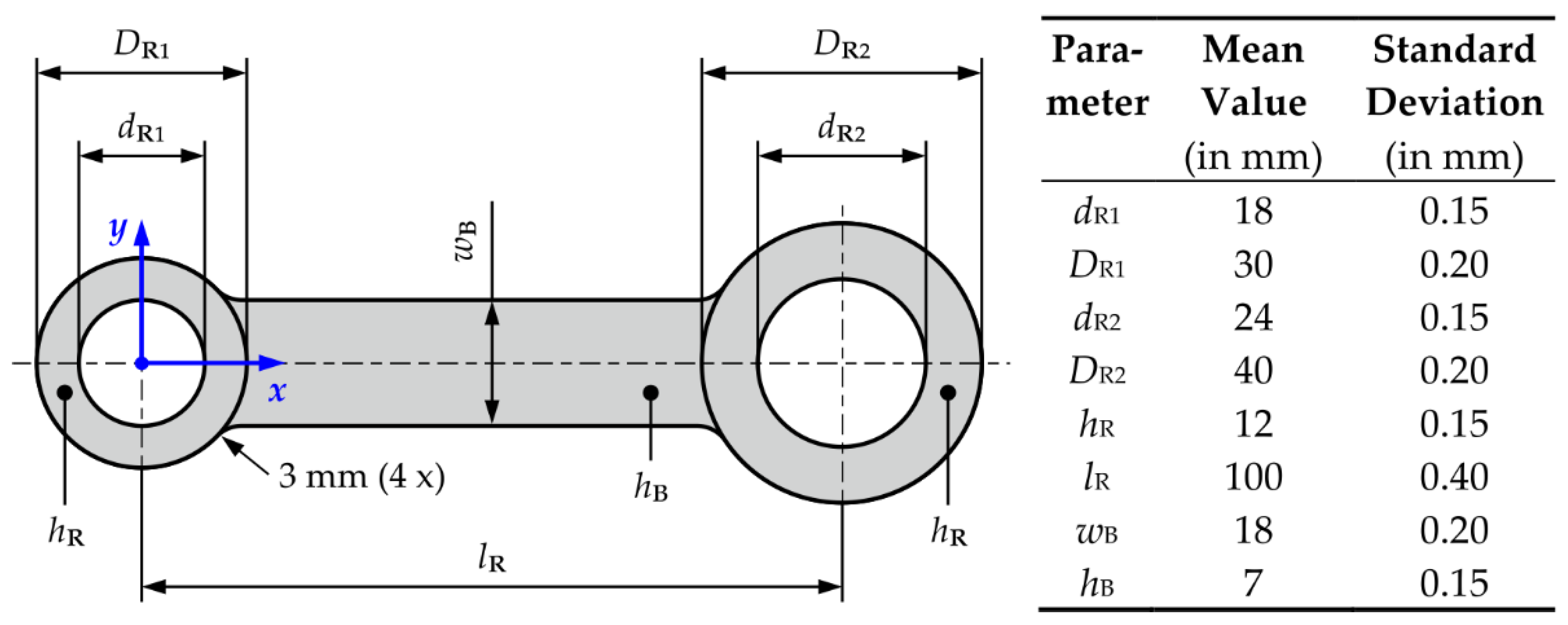
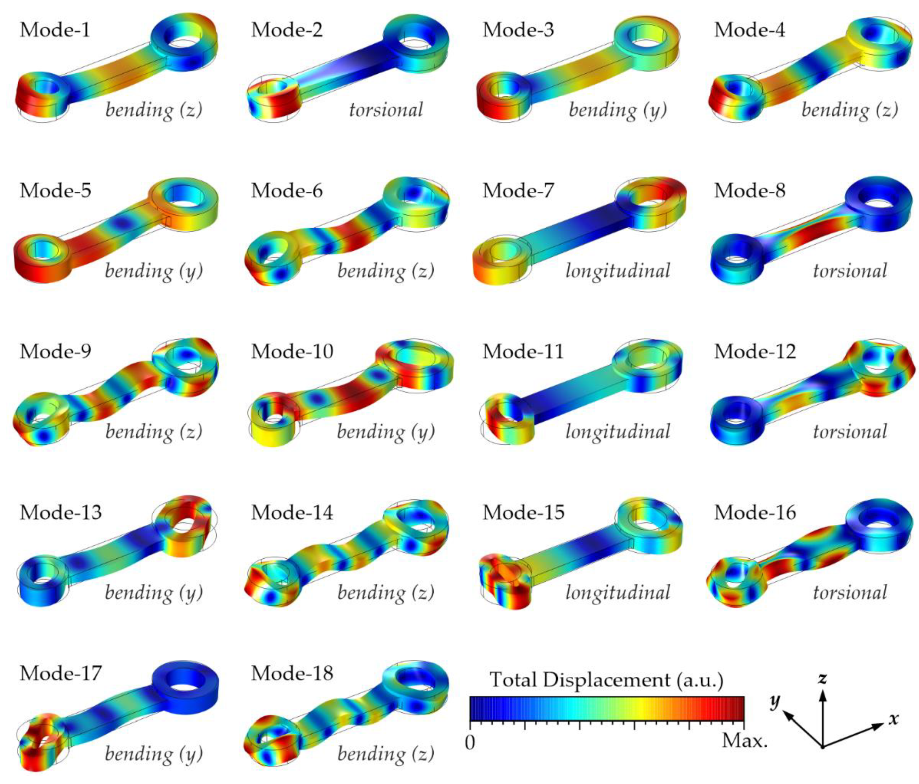
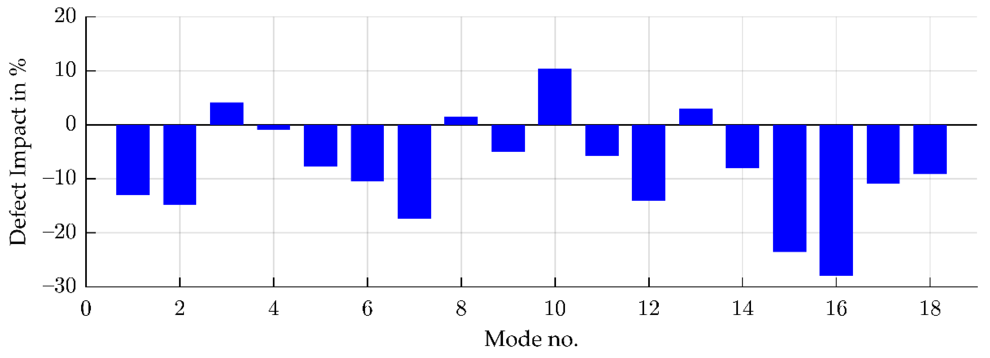
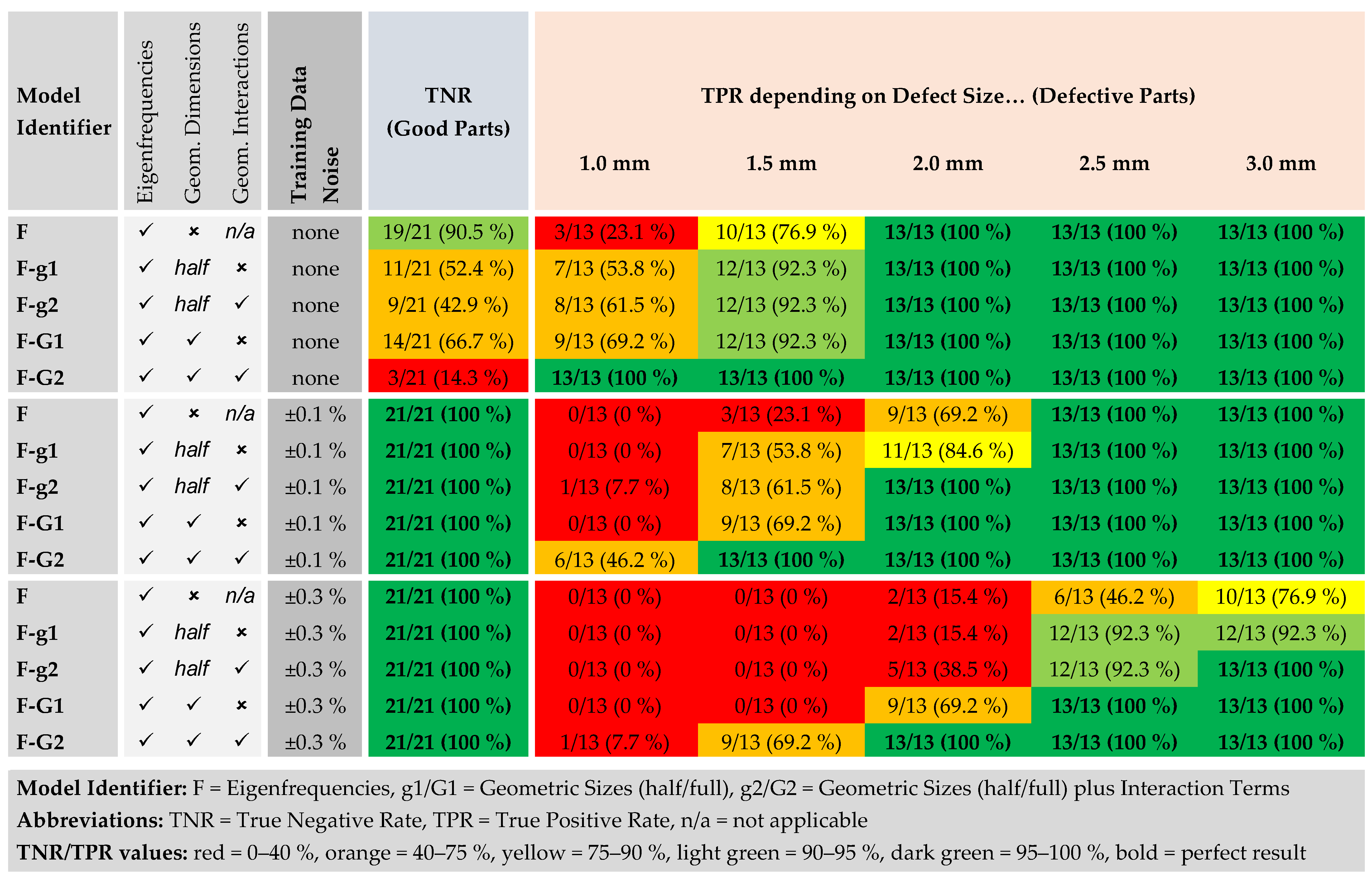
Table 1.
Statistics to characterize the connecting rod eigenfrequencies with regard to the frequencies in undamaged case, the frequency variations caused by geometric part-to-part variations, and the impact of a through-hole with 2 mm in diameter being central within the bar area.
Table 1.
Statistics to characterize the connecting rod eigenfrequencies with regard to the frequencies in undamaged case, the frequency variations caused by geometric part-to-part variations, and the impact of a through-hole with 2 mm in diameter being central within the bar area.
| Mode no. | Frequency without Defect | Geometry-Induced Standard Deviation | Frequency Shift due to a Central 2 mm Defect | ||
|---|---|---|---|---|---|
| (in Hz) | (in Hz) | (in %) | (in Hz) | (in %) | |
| 1 | 1760 | 45.3 | 2.58 | −5.9 | −0.34 |
| 2 | 3619 | 93.9 | 2.59 | −13.9 | −0.38 |
| 3 | 3705 | 56.0 | 1.51 | 2.3 | 0.06 |
| 4 | 5099 | 102.5 | 2.01 | −1.1 | −0.02 |
| 5 | 8974 | 98.0 | 1.09 | −7.5 | −0.08 |
| 6 | 10,292 | 141.6 | 1.38 | −15.0 | −0.15 |
| 7 | 12,032 | 100.1 | 0.83 | −17.4 | −0.14 |
| 8 | 13,802 | 156.1 | 1.13 | 2.2 | 0.02 |
| 9 | 16,507 | 156.2 | 0.95 | −7.8 | −0.05 |
| 10 | 17,083 | 146.8 | 0.86 | 15.2 | 0.09 |
| 11 | 18,797 | 148.3 | 0.79 | −8.5 | −0.05 |
| 12 | 20,303 | 140.0 | 0.69 | −19.8 | −0.10 |
| 13 | 21,186 | 164.3 | 0.78 | 4.8 | 0.02 |
| 14 | 22,399 | 202.5 | 0.90 | −16.3 | −0.07 |
| 15 | 26,471 | 196.6 | 0.74 | −46.2 | −0.17 |
| 16 | 26,727 | 230.6 | 0.86 | −64.6 | −0.24 |
| 17 | 28,356 | 265.0 | 0.93 | −28.8 | −0.10 |
| 18 | 29,125 | 262.9 | 0.90 | −24.3 | −0.08 |
Table 2.
Correction factors for adapting FEM eigenfrequencies to ART data.
| Mode no. | Correction Factor | Mode no. | Correction Factor | Mode no. | Correction Factor |
|---|---|---|---|---|---|
| 1 | 1.0272 | 7 | 1.0203 | 13 | 1.0202 |
| 2 | 1.0073 | 8 | 1.0089 | 14 | 1.0122 |
| 3 | 1.0238 | 9 | 1.0148 | 15 | 1.0199 |
| 4 | 1.0256 | 10 | 1.0183 | 16 | 1.0098 |
| 5 | 1.0196 | 11 | 1.0175 | 17 | 1.0178 |
| 6 | 1.0210 | 12 | 1.0120 | 18 | 1.0125 |
Publisher’s Note: MDPI stays neutral with regard to jurisdictional claims in published maps and institutional affiliations. |
© 2022 by the authors. Licensee MDPI, Basel, Switzerland. This article is an open access article distributed under the terms and conditions of the Creative Commons Attribution (CC BY) license (https://creativecommons.org/licenses/by/4.0/).
Share and Cite
MDPI and ACS Style
Heinrich, M.; Valeske, B.; Rabe, U. Efficient Detection of Defective Parts with Acoustic Resonance Testing Using Synthetic Training Data. Appl. Sci. 2022, 12, 7648. https://doi.org/10.3390/app12157648
AMA Style
Heinrich M, Valeske B, Rabe U. Efficient Detection of Defective Parts with Acoustic Resonance Testing Using Synthetic Training Data. Applied Sciences. 2022; 12(15):7648. https://doi.org/10.3390/app12157648
Chicago/Turabian StyleHeinrich, Matthias, Bernd Valeske, and Ute Rabe. 2022. "Efficient Detection of Defective Parts with Acoustic Resonance Testing Using Synthetic Training Data" Applied Sciences 12, no. 15: 7648. https://doi.org/10.3390/app12157648
Note that from the first issue of 2016, this journal uses article numbers instead of page numbers. See further details here.