
Machine Learning Prediction of Turning Precision Using Optimized XGBoost Model


1
Department of Intelligent Automation Engineering, National Chin Yi University of Technology, Taichung City 41170, Taiwan
2
Department of Mechanical Engineering, National Chung Cheng University, Chiayi 62102, Taiwan
3
Advanced Institute of Manufacturing with High-Tech Innovations (AIM-HI), National Chung Cheng University, Chiayi 62102, Taiwan
*
Author to whom correspondence should be addressed.
Appl. Sci. 2022, 12(15), 7739; https://doi.org/10.3390/app12157739
Submission received: 25 June 2022
/
Revised: 21 July 2022
/
Accepted: 25 July 2022
/
Published: 1 August 2022
(This article belongs to the Special Issue Human-Computer Interactions 2.0)
Abstract
:The present study proposes a machine learning approach for optimizing turning parameters in such a way as to maximize the turning precision. The Taguchi method is first employed to optimize the turning parameters, and the experimental results are then used to train three machine learning models to predict the turning precision for any given values of the input parameters. The model which shows the best prediction performance (XGBoost) is further improved through the use of a synthetic minority over-sampling technique for regression with Gaussian noise (SMOGN) and four different optimization algorithms, including center particle swarm optimization (CPSO). Finally, the performances of the various models are evaluated and compared using the leave-one-out cross-validation technique. The experimental results show that the XGBoost model, combined with SMOGN and CPSO, provides the best performance, and is a useful tool for predicting the machining error of turning. The method can also reduce the cost of obtaining the optimized turning parameters corresponding with the predicted machining error.
1. Introduction
Advances in machine tool technology make possible the creation of parts with tolerances as fine as ±0.0025 mm. Thus, precision machining plays a key role in fabricating many of the critical tight-tolerance components used in the military, electronics, aerospace, and medical industries nowadays. However, the success of precision machining methods still relies on the appropriate determination of the machining parameters. In the past, the optimal processing parameters were determined mainly by operator experience, or through a process of trial-and-error. However, such an approach is not only time-consuming, expensive, and subjective, but also offers no guarantee of finding the optimal solution. Furthermore, the knowledge learned in this way is not easily documented and shared with others. Thus, to realize the goals of high efficiency, high precision, and low cost, precision machining requires faster and more systematic approaches for identifying the optimal processing parameters.
Computer numerical control (CNC) machines are widely used throughout the manufacturing industry. CNC turning machines have many advantages for mass production, including a high speed, high precision, excellent repeatability, minimal manual intervention, and good potential for automation.
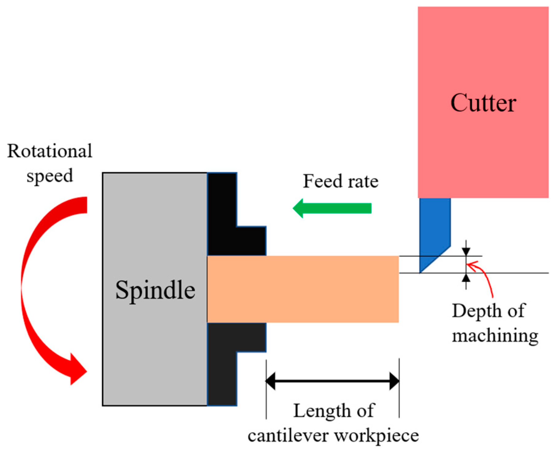
The cutting behavior of turning is determined by two components: the toolpath and the feed rate [1]. The “toolpath” is the trace on the workpiece that the cutter moves along, while the “feed rate” is the speed at which the cutter moves over the surface of the workpiece. When cutting metals, the machining quality is affected by two main types of factors, namely human and environmental. In most cases, the environmental factors, e.g., the age and condition of the machine, the machining temperature, the workpiece-material properties, and so on, are difficult to control. Accordingly, in attempting to improve the quality of the CNC machining process, many studies have focused on the problem of controlling the human factors, in particular, the settings assigned by the operator or designer of the machining parameters, such as the machining depth, rotational speed, feed rate, and cantilever cutting length. The machining depth has a direct effect on the cutting force exerted on the cutter. An excessive force may cause vibration of the cutter, which not only causes tool wear, but also significantly decreases the machining quality. The rotational speed and feed rate govern the speed at which the cutter moves over the workpiece. In general, a higher rotational speed and/or feed rate increases the rate at which the material is removed from the workpiece. However, an excessive speed may increase the cutting force, while a low speed increases the contact time between the cutter and the workpiece, and may thus result in the production of scratches. Finally, an excessive cantilever cutting length reduces the stability of the cutter at the contact point between the tip and the workpiece, and may therefore degrade the precision of the machining process. Hence, it is essential that all four machining parameters be optimized in order to ensure the quality and precision of the turning process.
Su et al. [2] presented a multi-objective optimization framework based on the robust Taguchi experimental design method, the grey relational analysis (GRA), and the response surface methodology (RSM) for determining the optimal cutting parameters in the turning of AISI 304 austenitic stainless steel. It was shown that, given the optimal settings of the turning parameters, the surface roughness (Ra) was reduced by 66.90%, and the material removal rate (MRR) was increased by 8.82%. Furthermore, the specific energy consumption (SEC) of the turning process was reduced by 81.46%. Akkus and Yaka [3] conducted a series of experiments to investigate the optimal cutting speed, feed rate, and depth of cut for the turning of Ti6Al4V titanium alloy. The optimality of the turning parameters was evaluated by examining their effects on surface roughness, vibration energy, and energy consumption. In general, the results revealed that the quality of the machining outcome was governed mainly by the feed rate. Zhou He et al. [4] proposed a genetic-gradient boosting regression tree (GA-GBRT) model, and used cutting speed, feed rate, and depth of cut as inputs to predict the surface roughness of milling, and then matched AISI 304 stainless steel for the cutting experiment. The results showed that the best processing parameters with the highest efficiency and best quality could be obtained based on the GA-GBRT model. Wu et al. [5] predicted the surface roughness when milling Inconel 718 through the Elman neural network according to the cutting conditions, vibration, and current signals during cutting, and then took the maximum cutting efficiency as the consideration and used the particle swarm optimization (PSO) algorithm to optimize cutting parameters. Sivalingam et al. [6] conducted the turning of Hastelloy X materials with PVD Ti-Al-N tools in different machining environments, and evaluated the cutting performances according to the cutting force, surface roughness, and cutting temperature caused by different cutting conditions. They found that the moth-flame optimization (MFO) algorithm could be applied to match the multiple linear regression models (MLRM) model to select the best processing parameters.
In response to the rise of artificial intelligence, this paper uses machine learning methods to predict turning machining error. Before using the machine learning method, a database of machining parameters and corresponding machining errors must be established to train the model. Due to the huge number of permutations and combinations of processing parameters, it is important to improve the efficiency of data collection. For this reason, this paper uses the Taguchi method to design the experiment, which can collect the most comprehensive data with the least number of experiments.
Machine learning [7] has proven effective in solving many problems which require extensive experimentation to obtain reliable results, or which involve such massive volumes of data that they cannot realistically be solved by manual analysis. Supervised machine learning models use a labelled dataset to learn the mapping function which most accurately describes the relationship between the input variables and the output (or outputs). Having trained the model, it is tested using a testing dataset and predicts the output accordingly. Such models have been widely applied for face detection, stock price prediction, spam detection, risk assessment, and so on. They have also been used to solve various problems in the field of smart manufacturing. For example, Lu et al. [8] studied the use of the group method of data handling (GMDH) model to predict the surface roughness of micro-milling LF21 antenna. The spindle speed and feed rate were used as model inputs, and the surface roughness was the output. The prediction accuracy could reach an average relative error of 13.92%, the maximum relative error was 21.22%, and finally, the best cutting parameters were found through the prediction results. Chen et al. [9] used a back-propagation neural network (BPNN) to predict the surface roughness of a milling workpiece. The model inputs were the depth of cut, feed rate, spindle speed and milling distance. The prediction accuracy was expressed by the root-mean-square-error (RMSE), which could reach 0.008, and analyzed the influence of various parameters on the surface roughness. The experimental results showed that the feed rate had the greatest influence on the surface roughness. Benardos and Vosniakos, et al. [10] used an artificial neural network (ANN) model based on the Levenberg–Marquardt (LM) training algorithm to predict the surface roughness in CNC face milling. In the proposed approach, the training and testing data were obtained using the Taguchi design of experiment (DoE) method based on seven control factors, namely the depth of cut, the feed rate per tooth, the cutting speed, the engagement and wear of the cutting tool, the cutting fluid, and the cutting force. It was shown that the trained model achieved a mean square error (MSE) of just 1.86% for the surface roughness of the milled component. Cus and Zuperl [11] developed an ANN for predicting the optimal cutting conditions subject to technological, economic, and organizational constraints. Asiltürk and Çunkaş [12] combined an ANN model and a regression analysis technique to predict the surface roughness of turned AISI 1040 steel. The model was trained using three different algorithms, namely back-propagation, scaled conjugate gradient (SCG), and Levenberg–Marquardt (LM). The results showed that the ANN model trained with the SCG algorithm provided a significantly better prediction accuracy than that obtained from a traditional, regression-based model. Pontes et al. [13] used the Taguchi DOE method to optimize the parameters of a radial base function (RBF) model for predicting the mean value of the surface roughness (Ra) of AISI 52,100 hardened steel in hand-turning processes. In general, the results confirmed that the use of the DOE approach to obtain the training data required to optimize the RBF model was far more efficient than traditional trial-and-error methods. The above studies focus mainly on the effects of the depth of cut, feed rate, and cutting speed on the surface roughness of machined components. However, besides the surface roughness, the machining error of the machining outcome is also extremely important, particularly for tight-tolerance components. The application of machine learning to the optimization of the cutting parameters is generally utilized by an ANN model [11,12]. However, such models, which have a simple structure consisting of an input layer, one or more hidden layers, and an output layer, achieve only a relatively poor prediction performance for machining precision. Accordingly, the present study examines the performance of three different tree-based machine learning (ML) models in predicting the precision of the turning process, namely random forest, XGBoost, and decision tree. For each model, the data required for training purposes are obtained using the Taguchi DOE method [14] based on four turning parameters: the machining depth, the rotational speed, the feed rate, and the cantilever cutting length. The model which shows the best prediction performance is further enhanced through the use of an over-sampling technique and four different optimization algorithms, namely genetic algorithm (GA), grey wolf (GW), PSO, and center particle swarm optimization (CPSO). Finally, the performances of the various models are evaluated and compared using the leave-one-out cross-validation technique.
In response to the rapid development of present technology, the requirements for product quality are also increasing, and the quality is closely related to the processing parameters. At present, there is no systematic method for the optimization of processing parameters in the industry, and most of them rely on empirical rules to overcome, but the disadvantages are that they are time-consuming and difficult to inherit techniques. In terms of research methods, in the past, it was necessary to rely on methods such as analyzing the structural characteristics of the machine or analyzing the cutting behavior in order to find suitable parameters more efficiently, but it was difficult and more expensive. Therefore, this paper proposes a kind of parameter optimization method to improve this problem. This method is to use the Taguchi method with the machine learning method for parameter optimization. In this paper, the Taguchi method and oversampling techniques are applied to improve the efficiency of data collection. Machine learning methods and optimization algorithms are then used to estimate the turning accuracy. The remainder of this paper is organized as follows: Section 2 briefly describes the setup of the Taguchi DOE method employed in the present study; Section 3 introduces the details of each of the major components of the proposed methodology, including the data preprocessing step, the ML models, the oversampling technique, and the optimization algorithms; Section 4 presents and discusses the experimental results; and finally, Section 5 provides some brief concluding remarks.
2. System Architecture
Figure 1 illustrates the four machining parameters considered in the present study, namely the depth of machining, the rotational speed, the feed rate, and the length of cantilever workpiece. The machining error is defined as the difference between the actual size and ideal size of diameter of a machined workpiece. The parameters have both individual and interactive effects on the precision of the machining process. Consequently, determining their respective impacts on the machining precision is challenging when using traditional trial-and-error methods. Accordingly, in the present study, the individual and interactive effects of the four parameters are investigated using the Taguchi DOE method, which allows for the optimal solution to be obtained with the minimal number of experiments. In the Taguchi method, the experiments are arranged in an orthogonal array (OA), where the configuration of this array depends on the number of control factors and level settings to be considered in the optimization process. In the present study, the aim is to investigate the effects of four machining parameters on the machining precision. Hence, the Taguchi experiments involve four control factors. Furthermore, each control factor is assigned three level settings, where these level settings are determined in accordance with the capabilities of the CNC machine used in the DOE trials (see Table 1). Accordingly, the experiments were configured in an L9 (34) OA containing nine experimental runs.
3. Proposed Method
In the present study, the effects of the four machining parameters on the turning precision were predicted using a supervised MK model. Most supervised-learning problems can be categorized as either “classification” problems or “regression” problems. Classification problems involve predicting a discrete valued output, such as a number or a certain species. By contrast, regression problems involve predicting a continuous valued output, such as stock market movement or the price of goods. The present study considered a regression-type problem, in which the aim was to predict the machining error of the turning process, given a knowledge of the settings assigned to the four machining parameters. The data required to train the ML model were obtained from the Taguchi DOE factorial design described in the previous section, where the level settings for the four machining parameters are listed in Table 2.
The machining error is calculated by the following equation:
where Dtarget is the diameter of the turning target size and Dmeasured is the diameter of the measured value after the turning process.
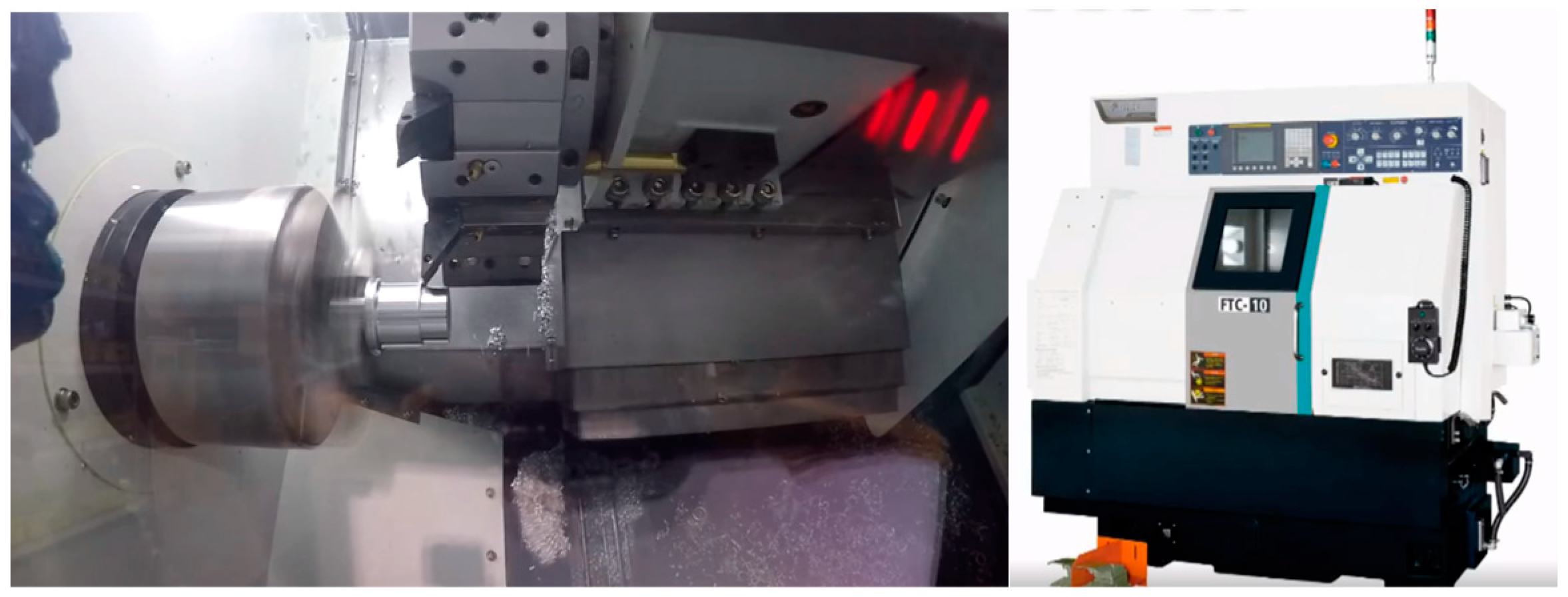
The turning experiments were performed on a Feeler turning machine (model: FTC-10), as shown in Figure 2, using cylindrical S45C medium carbon steel specimens. The specifications of the workpiece and cutting tool are shown in Table 3.
Prior to constructing the ML model, the experimental data obtained from the Taguchi experiments were pre-processed in order to accelerate the convergence of the training process and improve the prediction accuracy. Data pre-processing was performed using the min–max normalization [15] technique. In other words, the minimum and maximum values of each variable in the dataset were mapped to 0 and 1, respectively, and all the other values in between were scaled accordingly within the range of [0, 1]. In other words, the normalization process was performed as
where is the value after normalization and xmax, xmin, and x are the maximum, minimum, and original values, respectively. The normalization process is illustrated schematically in Figure 3.
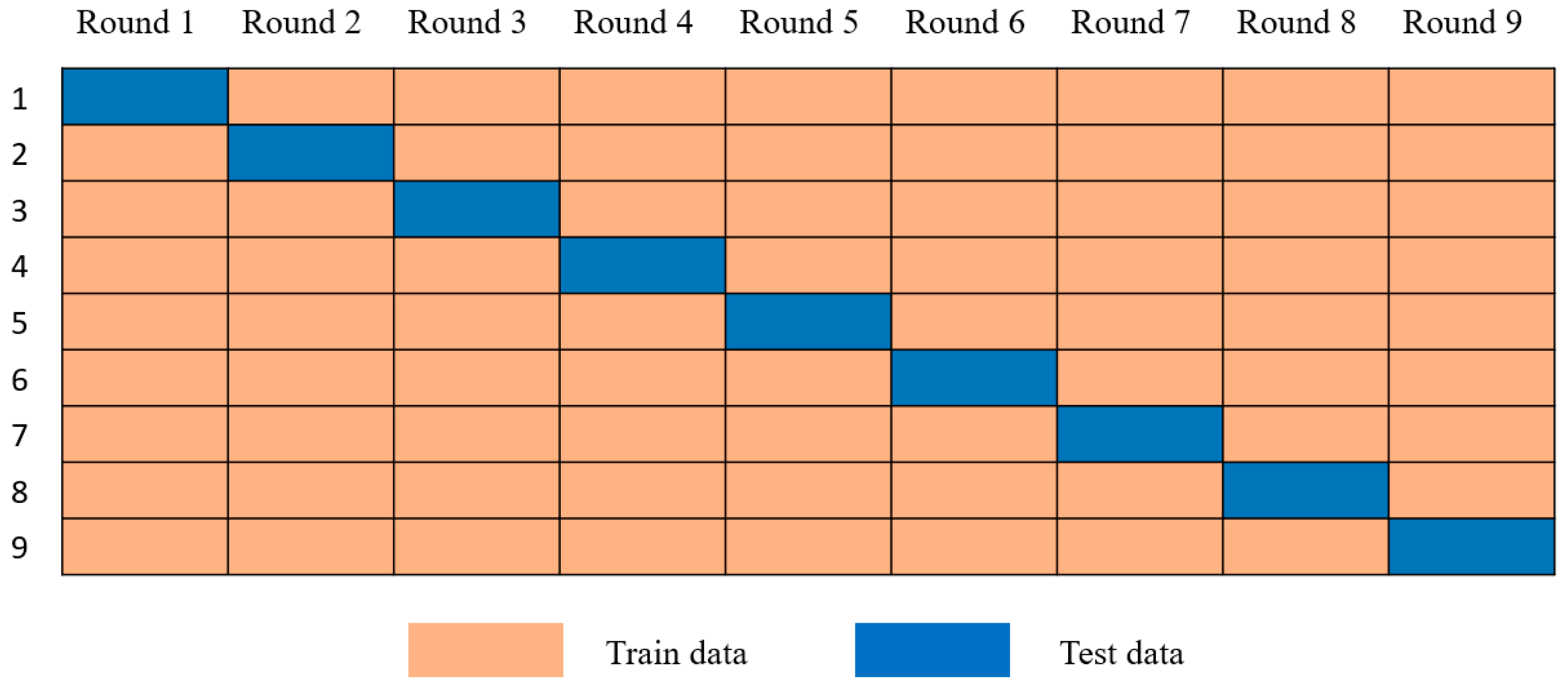
Following data processing, the model was trained and tested using the leave-one-out cross-validation technique [16]. Briefly, one data sample in the dataset was taken as an assessment set (i.e., a testing set), and all the other data samples were taken as a training set. The process was repeated until every data sample in the dataset had been taken as the assessment set once. As shown in Table 2, the Taguchi DOE design involved nine experimental runs. In other words, the Taguchi experiments generated nine data samples, with each sample consisting of the values assigned to the four machining parameters and the corresponding machining precision. Accordingly, the leave-one-out procedure was repeated nine times, as shown in Figure 4, with the prediction accuracy calculated each time.
The present study considered three ML models: random forest (RF), XGBoost (XGB), and decision tree (DT). Having evaluated the prediction performance of all three models, the model with the best performance was further improved using a synthetic minority over-sampling technique for regression with Gaussian noise (SMOGN) and four different optimization algorithms: genetic algorithm (GA), grey wolf (GW), particle swarm optimization (PSO), and center particle swarm optimization (CPSO). The prediction performances of the various models were then evaluated and compared. The details of the ML models, oversampling technique, and optimization algorithms are provided in the following sections.
3.1. Random Forest
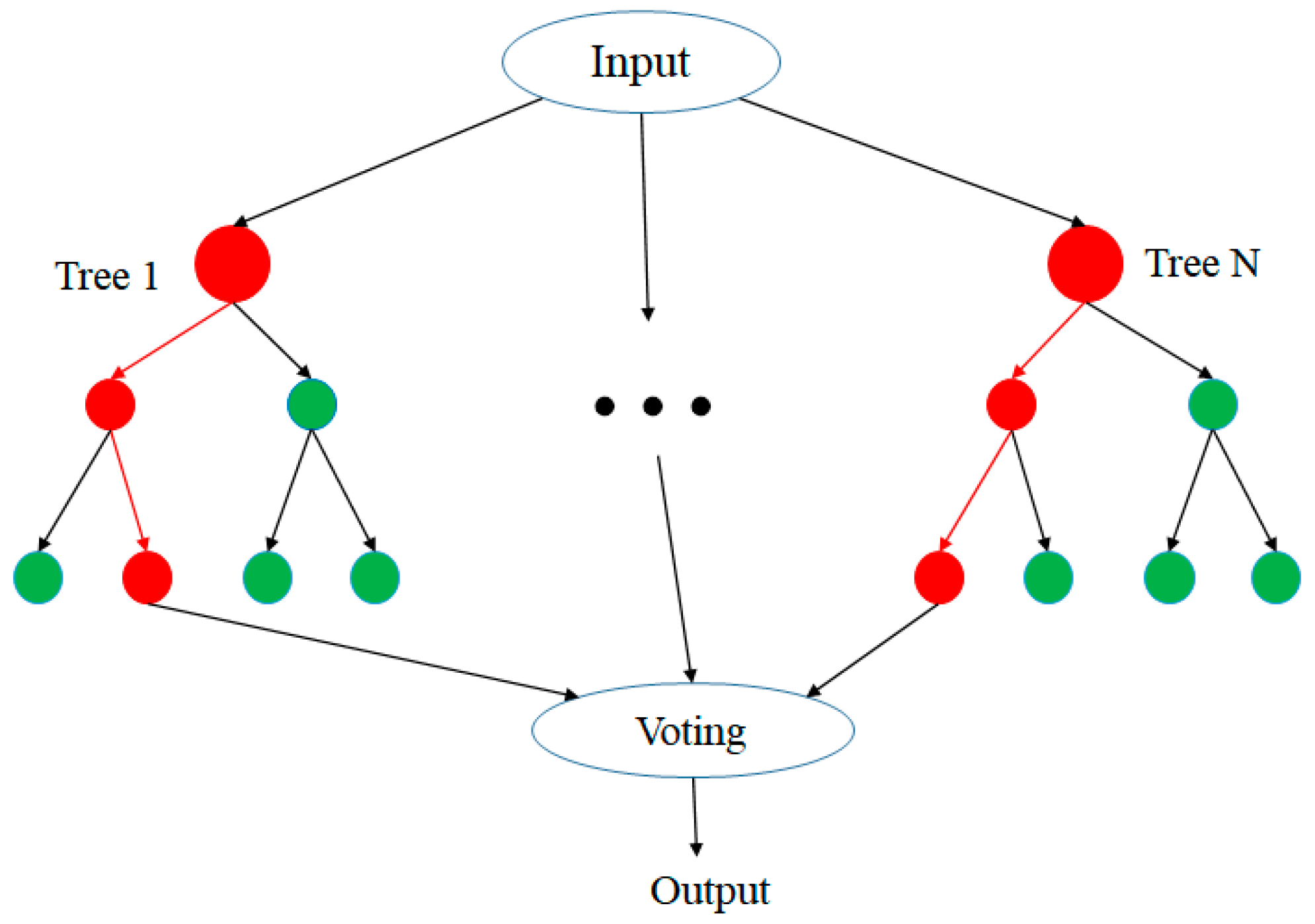
Random forest (RF) [17] combines the strengths of the bagging and decision tree algorithms, as shown in Figure 5. Bagging is used first to generate randomly distributed training data, and this data is then randomly assigned to multiple decision trees for training purposes. Since each decision tree uses different training data, each trained decision tree is different from the others. The weight of each decision tree is thus obtained via majority voting. As the training and testing process proceeds, the weaker decision trees are gradually combined to construct a stronger model with a better prediction performance.
3.2. XGBoost
Extreme gradient boosting (XGBoost or XGB) [18] combines the strengths of bagging and boosting, as shown in Figure 6. In particular, an additive model is first constructed, consisting of multiple base models. A new tree is then added to the model in order to correct the error produced by the previous tree, thereby improving the overall strength of the model. The process proceeds iteratively in this way until either no further improvement is obtained over a specified number of epochs, or the number of trees in the XGBoost structure reaches the maximum prescribed number.
In the present study, the maximum depth of the tree structure was set as 500, the number of samples was set as 1000, the learning rate was set as 0.3, and the booster was set as “gbtree”.
3.3. Decision Tree
The decision tree (DT) model [19] can be used to solve both classification and regression problems. In the present study, the model was used to solve the regression problem of predicting the turning precision based on the values of the four machining parameters. As shown in Figure 7, the DT structure consisted of three types of nodes: a root node, multiple interior nodes, and several output nodes. The root node represented the entire sample, while the interior nodes represented the features of the data set and the leaf nodes represented the regression outputs. Moreover, the branches between the nodes represented the decision rules (formulated as True or False). Briefly, each data point in the dataset was run through the tree until it reached an output node. The final prediction result was then obtained by computing the average value of the dependent variable at each node.
In this study, the depth of the DT structure was set as 10, the parameter controlling the randomness of the estimator was set as 0, and the feature split randomness criterion was set as “best” (meaning that the DT chose the split preferably based on the most important feature).
3.4. Oversampling
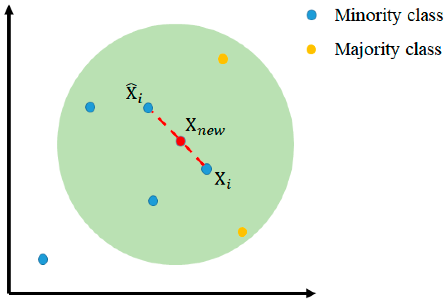
As described above, each of the three models was trained and tested using the leave-one-out cross-validation method. The best model was then further improved using the synthetic minority over-sampling technique for regression with Gaussian noise (SMOGN) [20]. In general, the purpose of oversampling is to overcome the problem of data imbalance in the dataset and/or insufficient available data. To preserve the original data features in the dataset, the data instances with few but important features are first identified. Synthetic data with similar features are then created, such that the final dataset contains a balanced number of features. In implementing the oversampling method, the sampling factor is set in accordance with the imbalance proportion of the data. In addition, the k-NN algorithm is applied to each sample X in the minority class. In particular, the distances between the sample and all the other samples in the same minority class are calculated in order to find the k minority class samples that are the closest to X. One of the minority class examples is then randomly selected and inserted into the following equation:
where is a random factor with a value in the interval of [0, 1] and is the minority class example selected (see Figure 8).
3.5. Model Optimization
Following the over-sampling process, optimization algorithms [21] were applied to further tune the parameters of the ML model. Four algorithms were considered, namely GA, GW, PSO and CPSO. The details of each algorithm are described in the following.
The genetic algorithm (GA) optimizer [22] was a randomized search algorithm which imitated the processes of selection and reproduction in nature. The algorithm commenced by constructing an initial population of potential candidate solutions, where each candidate was encoded in the form of a string. A set of these candidates was then selected as the initial guessed values, and selection, crossover, and mutation operations were performed based on the fitness of these guessed values in order to create a new population of improved candidate solutions. The algorithm iterated in this way until the specified termination criteria were satisfied, at which point the candidate with the best fit was decoded and taken as the optimal solution. Figure 9 illustrates the basic workflow of the GA algorithm.
The grey wolf (GW) optimizer [23] is an intelligent optimization algorithm that mimics the group hunting behavior of grey wolves, and involves three main steps, namely, establishing hierarchy, encircling, and attacking. As shown in Figure 10, three solutions (alpha, beta, and delta) are first selected as the best solutions among the initial population. In each iteration, the position of the prey (i.e., the optimal solution) is updated according to the positions of these wolves, based on
where t is the current iteration; A and C are the auxiliary coefficient vectors; is the position vector of the prey; and is the current position vector of the wolves. drops from 2 to 0 as the iteration process proceeds, and and are random vectors in the interval of [0, 1]. In the hunting process, when > 1, the wolves diverge. By contrast, when < 1, they converge, and search a more localized area in order to pinpoint the prey.
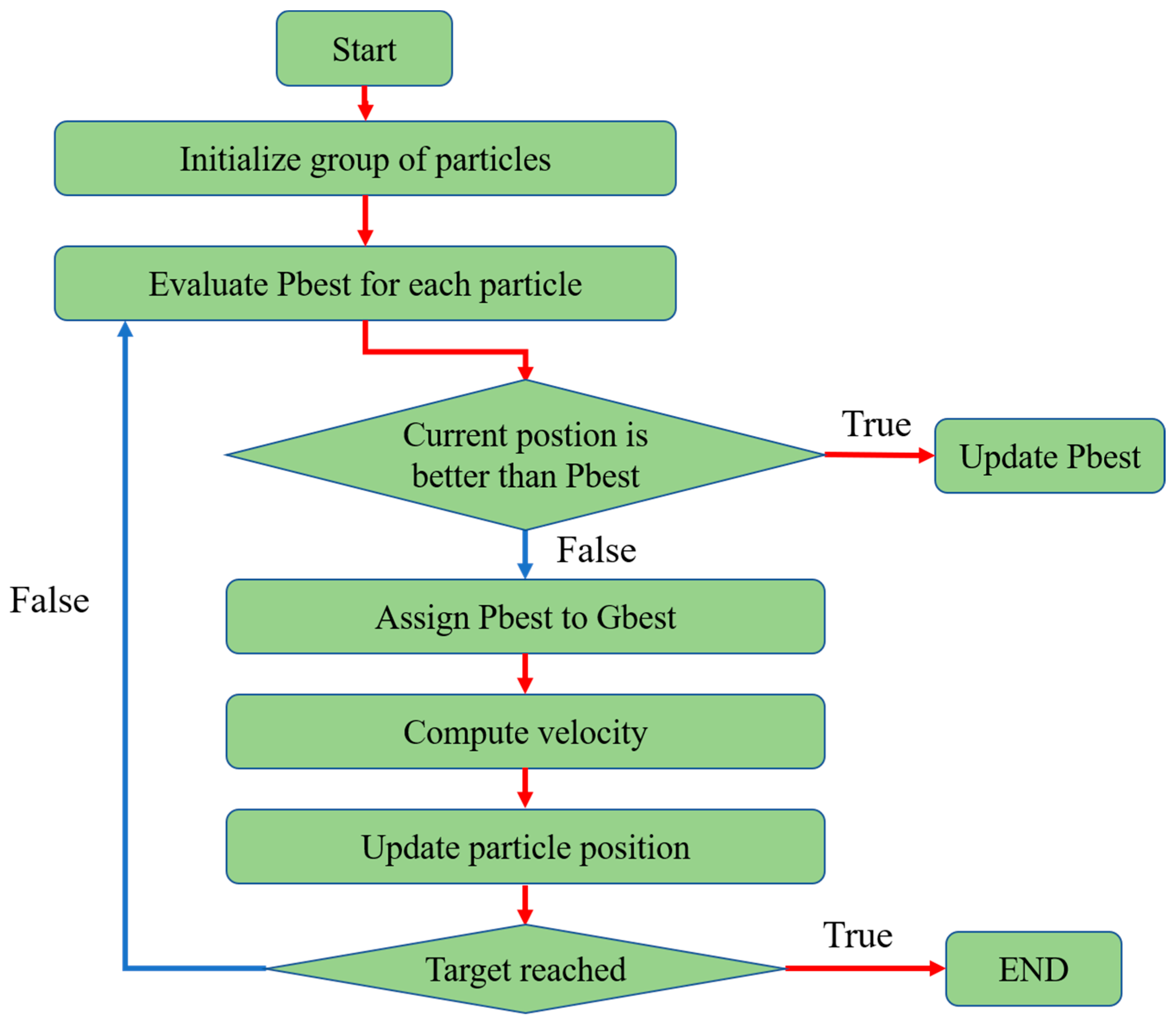
The particle swarm optimization (PSO) algorithm [24] encodes each candidate solution as a particle within the feasible search space, and gradually converges toward the optimal solution based on the individual and collective experiences of all the members of the swarm. As shown in Figure 11, the optimization process involves three iterative steps: (one) assigning the initial positions of all the particles and recording the position of the best solution among them, (two) calculating the acceleration vector for each particle and moving the particle to a new position, and (three) updating the personal best solutions of the individual particles and the global best solution. The related PSO equations are expressed as follows:
where is the velocity of individual i in the k-th iteration, is the weight, and are the acceleration constants, and and are random values in the interval [0, 1]. In addition, is the position of individual i in the k-th iteration, is the best position of individual i in each iteration, and is the best solution in the entire domain.
Center particle swarm optimization (CPSO) [25] is an extension of the PSO algorithm, and aims to reach the optimal solution more rapidly through the introduction of a center particle located in the middle of all the particles in the swarm (see Figure 12). The rationale for this approach lies in the fact that the center of the personal best solutions of all the particles is located closer to the best solution than the global best solution. Thus, in the CPSO algorithm, the position of the center particle is taken in place of the global best position in the original PSO algorithm in order to improve the convergence speed. The position of the center particle is computed as
where is the center position in the (k + 1)-th iteration, N is the number of particles in the swarm, and is the position of the i-th particle in the (k + 1)-th iteration.
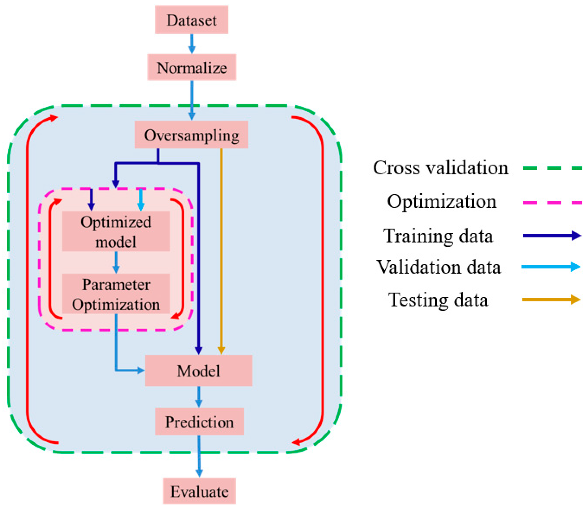
Figure 13 and Figure 14 show the training procedures for the single RF, XGBoost, and DT models, and the optimized models, respectively. As shown in Figure 13, the training process for the single models involves the following steps: (one) loading the data, (two) data normalization, (three) cross validation (separating the training set and test set), (four) model training, (five) prediction, and (six) prediction accuracy evaluation. Similarly, the main steps in the training process for the optimized models include: (one) loading the data, (two) data normalization, (three) cross validation, (four) oversampling, (five) model optimization, (six) model training using the optimized parameters, (seen) prediction, and (eight) prediction accuracy evaluation (see Figure 14).
4. Experimental Results
4.1. Performances of Different ML Models
As described in Section 3, the ML models were trained and tested using the leave-one-out cross-validation technique with nine data samples. For each testing process, the prediction performance of the model was evaluated using three different metrics: the root mean square error (RMSE), the mean absolute error (MAE), and the coefficient of determination ().
The RMSE computes the square root of the ratio of the square of the errors between the predicted values and the actual values over the number of data instances. The square relationship in the RMSE formula renders the metric sensitive to very large or very small errors. A larger RMSE indicates a poorer prediction performance, and vice versa. The mean absolute error (MAE) computes the sum of the absolute values of the differences between the actual values of the machining error and the predicted values. In other words, a smaller MAE indicates a better prediction accuracy, and vice versa.
Finally, the coefficient of determination ( or the score) is a statistical measure representing the proportion of variance in the dependent variable. In other words, it provides an indication of how well (or otherwise) the prediction model fits the actual data. The score has a value in the interval of [0, 1], where a value closer to 1 indicates a better fit of the prediction model.
The leave-one-out cross-validation process revealed that all of the trained single models (RF, XGBoost, and DT) had a poor prediction performance. However, among the three models, the best performance was obtained by the XGBoost model, with a RMSE of 0.007887, a MAE of 0.0067, and an score of 0.554. Accordingly, the XGBoost model was selected for further improvement using the SMOGN over-sampling method and four optimization algorithms.
Figure 15 shows the learning curves of the four optimizers. Note that in compiling the results, the RMSE values of the optimizers were taken as the fitness value, and once a better fitness value was found in the model optimization process, it was used in place of the best fitness value. In other words, a lower learning curve in Figure 15 indicates an improved optimization performance, and shows that the CPSO optimizer yields the best learning performance.
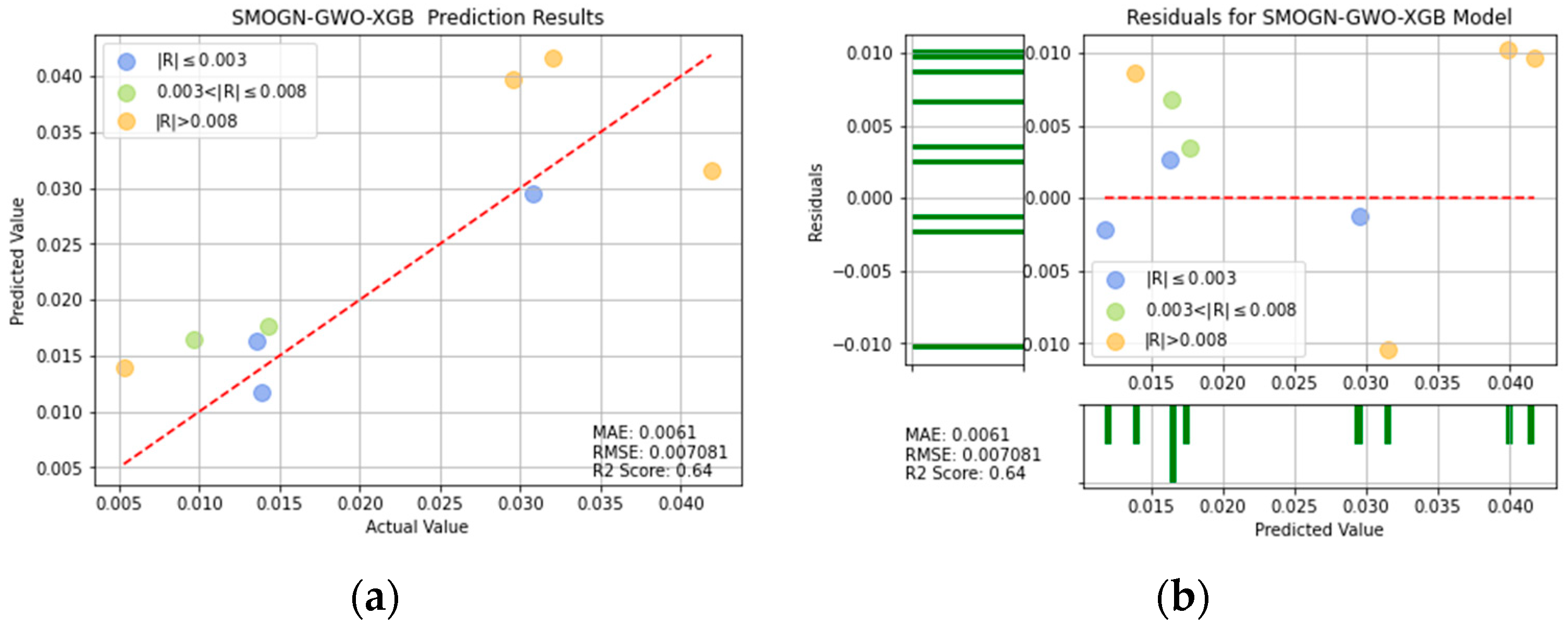
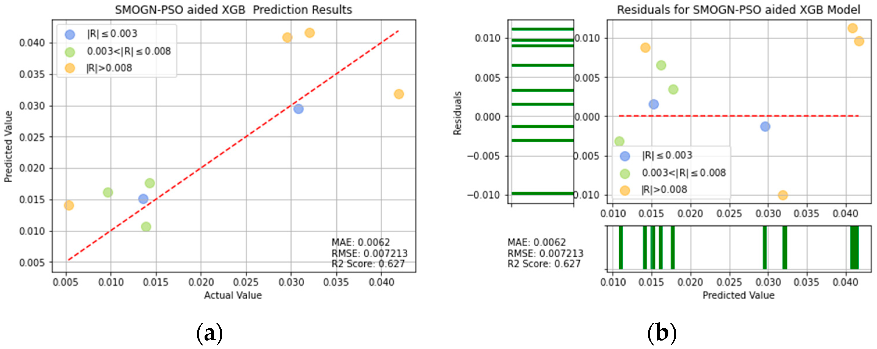
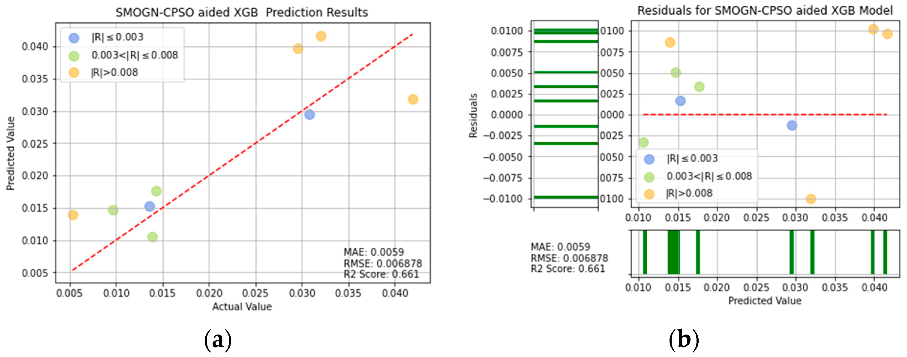
Figure 16, Figure 17, Figure 18, Figure 19, Figure 20, Figure 21 and Figure 22 show the prediction results obtained for the seven ML models (i.e., the three single models and the four over-sampled and optimized XGBoost models). For each model, the figures show both a direct comparison of the actual and predicted machining errors and the corresponding residual plot.
For ease of visualization and comparison, the prediction errors with a value greater than 0.008 in Figure 16, Figure 17, Figure 18, Figure 19, Figure 20, Figure 21 and Figure 22 are shown in orange, while those with a value between 0.003 and 0.008 are shown in green, and those with a value less than 0.003 are shown in blue. Thus, the prediction accuracy of each model can be crudely evaluated by the number of points of each color in the respective plots. A more quantitative evaluation of the performance of each model can be obtained from the corresponding RMSE, MAE, and values.
Figure 23 compares the predicted machining errors of the seven models with the actual machining error for each of the nine runs in the Taguchi OA. Overall, the results show that the SMOGN-CPSO-XGB model and SMOGN-GWO-XGB model yield the best fits with the actual prediction error in each run. By contrast, the RF model yields the poorest fit with the experimental data.
Table 4 lists the MAE, RMSE, and values of the seven models. In general, the results confirm the effectiveness of the SMOGN technique and optimization algorithms in improving the prediction performance, compared with that of the single models. Moreover, the results confirm that, among all of the models, the XGBoost model optimized with SMOGN and CPSO achieves the lowest MAE and RMSE values and the highest score.
The values of R2 for SMOGN-CPSO-XGB and SMOGN-GWO-XGB are 0.661 and 0.64, respectively. It can be seen that SMOGN-CPSO-XGB and SMOGN-GWO-XGB have better prediction effects than the others and perform a good performance, as shown in Table 4. If the two models of SMOGN-CPSO-XGB and SMOGN-GWO-XGB are compared by evaluating the three indicators of MAE, RMSE, and R2, the performances of MAE and R2 for SMOGN-CPSO-XGB model are significantly better than the SMOGN-GWO-XGB model. Accordingly, the SMOGN-CPSO-XGB model has the best predictive ability and effect for turning process. It is also shown that from the R2 value, the prediction effect of SMOGN-CPSO-XGB model is significantly higher than that of the decision tree model by 23%. In other words, the SMOGN-CPSO-XGB model is the best fitted model among the considered alternatives.
4.2. Confirmation Experiments for the Prediction of the SMOGN-CPSO-XGB Model
In Table 2, the optimized combination of parameters is A3B1C1D2, which means the depth of machining, rotational speed, feed rate, and length of cantilever workpiece are 1.0 mm, 2000 rpm, 0.15 mm/rev, and 60 mm, respectively. This set of parameters is then applied to be the input of the SMOGN-CPSO-XGB model, and the obtained predicted value of machining error is 0.005163 mm within 0.002 s. The result is the best of all values of machining error in Table 2. It is confirmed that the SMOGN-CPSO-XGB model is suitable for the prediction in the turning process.
If a set of experimental factors and levels designed by the Taguchi method are input arbitrarily, the predicted machining error of the workpiece can be accurately obtained through the SMOGN-CPSO-XGB model. For the industry, it is very important that when a certain processing parameter changes, the machining error change of the workpiece needs to be quickly understood, which can be used as a reference for parameter adjustment. It can also instantly understand the impact of machining parameter changes on the workpiece accuracy.
5. Conclusions
This study has proposed a machine learning approach for predicting the machining precision of the turning process based on the values assigned to the machining depth, rotational speed, feed rate, and cantilever cutting length, respectively. Based on the experimental results obtained from the Taguchi factorial design experiment, the contributions of this study are summarized as follows.
- (1).
- The XGBoost model yields a better prediction performance than the random forest model or decision tree model. It has further been shown that the prediction performance of the XGBoost model can be enhanced through the use of a synthetic minority over-sampling technique for regression with Gaussian noise (SMOGN) and a center particle swarm optimization (CPSO) algorithm.
- (2).
- According to the index of R2, it can be observed that the values of R2 for the SMOGN-CPSO-XGB and SMOGN-GWO-XGB models are 0.661 and 0.64, respectively. It reveals that the SMOGN-CPSO-XGB and SMOGN-GWO-XGB models have better prediction effects than the others and perform well.
- (3).
- For the comparison of performance for the SMOGN-CPSO-XGB and SMOGN-GWO-XGB models, it is evaluated by MAE, RMSE, and R2 to show that the performance of the SMOGN-CPSO-XGB model can achieve a MAE of 0.0059, and an R2 score of 0.661 is significantly better than the SMOGN-GWO-XGB model. Accordingly, the SMOGN-CPSO-XGB model has the best predictive ability and effect for turning process.
- (3).
- This study provides a rapid and reliable means of predicting the turning quality, optimizing the turning parameters or machining error in industrial settings without the need for time-consuming and expensive trial-and-error experiments.
Author Contributions
Conceptualization, C.-C.W.; methodology, C.-C.W.; software, P.-H.K.; validation, C.-C.W., P.-H.K. and G.-Y.C.; formal analysis, P.-H.K. and G.-Y.C.; investigation, C.-C.W.; writing—original draft preparation, C.-C.W., P.-H.K. and G.-Y.C.; writing—review and editing, C.-C.W.; visualization, C.-C.W.; supervision, C.-C.W.; project administration, C.-C.W.; funding acquisition, C.-C.W. All authors have read and agreed to the published version of the manuscript.
Funding
This research was funded by Ministry of Science and Technology in Taiwan, grant number MOST 110-2221-E-167-019.
Conflicts of Interest
The authors declare no conflict of interest.
References
- Stephenson, D.A.; Agapiou, J.S. Metal Cutting Theory and Practice; CRC Press: Boca Raton, FL, USA, 2018. [Google Scholar]
- Su, Y.; Zhao, G.; Zhao, Y.; Meng, J.; Li, C. Multi-objective optimization of cutting parameters in turning AISI 304 austenitic stainless steel. Metals 2020, 10, 217. [Google Scholar] [CrossRef] [Green Version]
- Akkuş, H.; Yaka, H. Experimental and statistical investigation of the effect of cutting parameters on surface roughness, vibration and energy consumption in machining of titanium 6Al-4V ELI (grade 5) alloy. Measurement 2021, 167, 108465. [Google Scholar] [CrossRef]
- Zhou, T.; He, L.; Wu, J.; Du, F.; Zou, Z. Prediction of surface roughness of 304 stainless steel and multi-objective optimization of cutting parameters based on GA-GBRT. Appl. Sci. 2019, 9, 3684. [Google Scholar] [CrossRef] [Green Version]
- Wu, T.Y.; Lin, C.C. Optimization of machining parameters in milling process of inconel 718 under surface roughness constraints. Appl. Sci. 2021, 11, 2137. [Google Scholar] [CrossRef]
- Sivalingam, V.; Sun, J.; Mahalingam, S.K.; Nagarajan, L.; Natarajan, Y.; Salunkhe, S.; Nasr, E.A.; Davim, J.P.; Hussein, H.M.A.M. Optimization of process parameters for turning Hastelloy x under different machining environments using evolutionary algorithms: A comparative study. Appl. Sci. 2021, 11, 9725. [Google Scholar] [CrossRef]
- Jordan, M.I.; Mitchell, T.M. Machine learning: Trends, perspectives, and prospects. Science 2015, 349, 255–260. [Google Scholar] [CrossRef] [PubMed]
- Lu, X.; Hou, P.; Luan, Y.; Sun, X.; Qiao, J.; Zhou, Y. Study on surface roughness of sidewall when micro-milling LF21 waveguide slits. Appl. Sci. 2022, 12, 5415. [Google Scholar] [CrossRef]
- Chen, C.H.; Jeng, S.Y.; Lin, C.J. Prediction and analysis of the surface roughness in CNC end milling using neural networks. Appl. Sci. 2022, 12, 393. [Google Scholar] [CrossRef]
- Benardos, P.; Vosniakos, G. Prediction of surface roughness in CNC face milling using neural networks and Taguchi’s design of experiments. Robot. Comput. Integr. Manuf. 2002, 18, 343–354. [Google Scholar] [CrossRef]
- Cus, F.; Zuperl, U. Approach to optimization of cutting conditions by using artificial neural networks. J. Mater. Process. Technol. 2006, 173, 281–290. [Google Scholar] [CrossRef]
- Asiltürk, İ.; Çunkaş, M. Modeling and prediction of surface roughness in turning operations using artificial neural network and multiple regression method. Expert Syst. Appl. 2011, 38, 5826–5832. [Google Scholar] [CrossRef]
- Pontes, F.J.; de Paiva, A.P.; Balestrassi, P.P.; Ferreira, J.R.; da Silva, M.B. Optimization of radial basis function neural network employed for prediction of surface roughness in hard turning process using Taguchi’s orthogonal arrays. Expert Syst. Appl. 2012, 39, 7776–7787. [Google Scholar] [CrossRef]
- Moganapriya, C.; Rajasekar, R.; Ponappa, K.; Venkatesh, R.; Jerome, S. Influence of coating material and cutting parameters on surface roughness and material removal rate in turning process using Taguchi method. Mater. Today Proc. 2018, 5, 8532–8538. [Google Scholar] [CrossRef]
- Kolarik, M.; Burget, R.; Riha, K. Comparing normalization methods for limited batch size segmentation neural networks. In Proceedings of the 2020 43rd International Conference on Telecommunications and Signal Processing (TSP), Milan, Italy, 7–9 July 2020. [Google Scholar] [CrossRef]
- Ko, A.H.R.; Cavalin, P.R.; Sabourin, R.; de Souza Britto, A. Leave-one-out-training and leave-one-out-testing hidden Markov models for a handwritten numeral recognizer: The implications of a single classifier and multiple classifications. IEEE Trans. Pattern Anal. Mach. Intell. 2009, 31, 2168–2178. [Google Scholar] [CrossRef] [PubMed]
- Prihatno, A.T.; Nurcahyanto, H.; Jang, Y.M. Predictive maintenance of relative humidity using random forest method. In Proceedings of the 2021 International Conference on Artificial Intelligence in Information and Communication (ICAIIC), Jeju Island, Korea, 13–16 April 2021. [Google Scholar] [CrossRef]
- Zhang, K.; Gu, C.; Zhu, Y.; Chen, S.; Dai, B.; Li, Y.; Shu, X. A novel seepage behavior prediction and lag process identification method for concrete dams using HGWO-XGBoost model. IEEE Access 2021, 9, 23311–23325. [Google Scholar] [CrossRef]
- Patil, S.; Kulkarni, U. Accuracy prediction for distributed decision tree using machine learning approach. In Proceedings of the 2019 3rd International Conference on Trends in Electronics and Informatics (ICOEI), Tirunelveli, India, 23–25 April 2019. [Google Scholar] [CrossRef]
- Branco, P.; Torgo, L.; Ribeiro, R.P. SMOGN: A pre-processing approach for imbalanced regression. In Proceedings of the First International Workshop on Learning with Imbalanced Domains: Theory and Applications, Skopje, Macedonia, 22 September 2017. [Google Scholar]
- Das, U.K.; Tey, K.S.; Seyedmahmoudian, M.; Mekhilef, S.; Idris, M.Y.I.; Deventer, W.V.; Horan, B.; Stojcevski, A. Forecasting of photovoltaic power generation and model optimization: A review. Renew. Sustain. Energy Rev. 2018, 81, 912–928. [Google Scholar] [CrossRef]
- Shin, Y.; Kim, Z.; Yu, J.; Kim, G.; Hwang, S. Development of NOx reduction system utilizing artificial neural network (ANN) and genetic algorithm (GA). J. Clean. Prod. 2019, 232, 1418–1429. [Google Scholar] [CrossRef]
- Nadimi-Shahraki, M.H.; Taghian, S.; Mirjalili, S. An improved grey wolf optimizer for solving engineering problems. Expert Syst. Appl. 2012, 166, 113917. [Google Scholar] [CrossRef]
- Sharif, M.; Amin, J.; Raza, M.; Yasmin, M.; Satapathy, S.C. An integrated design of particle swarm optimization (PSO) with fusion of features for detection of brain tumor. Pattern Recognit. Lett. 2020, 129, 150–157. [Google Scholar] [CrossRef]
- Yang, X.; Jiao, Q.; Liu, X. Center particle swarm optimization algorithm. In Proceedings of the 2019 IEEE 3rd Information Technology, Networking, Electronic and Automation Control Conference (ITNEC), Chengdu, China, 15–17 March 2019. [Google Scholar] [CrossRef]
Figure 1.
Schematic illustration of turning parameters.

Figure 2.
Feeler turning machine (Model: FTC-10) used in experiments.

Figure 3.
Conceptual representation of data normalization.

Figure 4.
Conceptual representation of leave-one-out procedure.

Figure 5.
Conceptual representation of random forest algorithm.

Figure 6.
Conceptual representation of the XGBoost algorithm.

Figure 7.
Conceptual representation of decision tree.

Figure 8.
Conceptual representation of the SMOGN algorithm.

Figure 9.
Conceptual representation of the GA algorithm.

Figure 10.
Conceptual representation of the GWO algorithm.

Figure 11.
Conceptual representation of the PSO algorithm.

Figure 12.
Conceptual representation of the CPSO algorithm.

Figure 13.
Single model training flowchart.

Figure 14.
Optimized model training flowchart.

Figure 15.
Learning curves of different optimizers.

Figure 16.
RF prediction results: (a) comparison of actual and predicted precision values, and (b) residual plot.
Figure 16.
RF prediction results: (a) comparison of actual and predicted precision values, and (b) residual plot.

Figure 17.
DT prediction results: (a) comparison of actual and predicted precision values, and (b) residual plot.
Figure 17.
DT prediction results: (a) comparison of actual and predicted precision values, and (b) residual plot.

Figure 18.
XGBoost prediction results: (a) comparison of actual and predicted precision values, and (b) residual plot.
Figure 18.
XGBoost prediction results: (a) comparison of actual and predicted precision values, and (b) residual plot.

Figure 19.
SMOGN-GA-XGB prediction results: (a) comparison of actual and predicted precision values, and (b) residual plot.
Figure 19.
SMOGN-GA-XGB prediction results: (a) comparison of actual and predicted precision values, and (b) residual plot.

Figure 20.
SMOGN-GW-XGB prediction results: (a) comparison of actual and predicted precision values, and (b) residual plot.
Figure 20.
SMOGN-GW-XGB prediction results: (a) comparison of actual and predicted precision values, and (b) residual plot.

Figure 21.
SMOGN-PSO-XGB prediction results: (a) comparison of actual and predicted precision values, and (b) residual plot.
Figure 21.
SMOGN-PSO-XGB prediction results: (a) comparison of actual and predicted precision values, and (b) residual plot.

Figure 22.
SMOGN-CPSO-XGB prediction results: (a) comparison of actual and predicted precision values, and (b) residual plot.
Figure 22.
SMOGN-CPSO-XGB prediction results: (a) comparison of actual and predicted precision values, and (b) residual plot.

Figure 23.
Prediction performance of different models.


Table 1.
Factor and standard.
| Level | 1 | 2 | 3 |
|---|---|---|---|
| Factor | |||
| A. Depth of machining (mm) | 0.1 | 0.5 | 1.0 |
| B. Rotational speed (rpm) | 2000 | 2300 | 2500 |
| C. Feed rate (mm/rev) | 0.15 | 0.2 | 0.25 |
| D. Length of cantilever workpiece (mm) | 40 | 60 | 80 |
Table 2.
Factor and standard. Experimental results by L9 orthogonal array.
| Case | A. Depth of Machining (mm) | B. Rotational Speed (rpm) | C. Feed Rate (mm/rev) | D. Length of Cantilever Workpiece (mm) | Machining Error (mm) |
|---|---|---|---|---|---|
| 1 | 0.1 | 2000 | 0.15 | 40 | 0.013617 |
| 2 | 0.1 | 2300 | 0.2 | 60 | 0.0308 |
| 3 | 0.1 | 2500 | 0.25 | 80 | 0.02955 |
| 4 | 0.5 | 2000 | 0.2 | 80 | 0.03207 |
| 5 | 0.5 | 2300 | 0.25 | 40 | 0.0419 |
| 6 | 0.5 | 2500 | 0.15 | 60 | 0.01425 |
| 7 | 1 | 2000 | 0.25 | 60 | 0.00961 |
| 8 | 1 | 2300 | 0.15 | 80 | 0.0053 |
| 9 | 1 | 2500 | 0.2 | 40 | 0.01391 |
Table 3.
Specifications of workpiece and cutting tool.
| Diameter of Workpiece (mm) | 30 |
| Length of Workpiece (mm) | 175 |
| Cutting Tool Length (mm) | 125 |
| Cutting Tool Weight (g) | 430 |
Table 4.
Performance metrics of various models.
| Model | MAE | RMSE | |
|---|---|---|---|
| Random Forest | 0.0107 | 0.012336 | −0.092 |
| Decision Tree | 0.0068 | 0.008034 | 0.537 |
| XGBoost | 0.0067 | 0.007887 | 0.554 |
| SMOGN-GA-XGB | 0.0064 | 0.007411 | 0.606 |
| SMOGN-GWO-XGB | 0.0061 | 0.007081 | 0.64 |
| SMOGN-PSO-XGB | 0.0062 | 0.007213 | 0.627 |
| SMOGN-CPSO-XGB | 0.0059 | 0.006878 | 0.661 |
Publisher’s Note: MDPI stays neutral with regard to jurisdictional claims in published maps and institutional affiliations. |
© 2022 by the authors. Licensee MDPI, Basel, Switzerland. This article is an open access article distributed under the terms and conditions of the Creative Commons Attribution (CC BY) license (https://creativecommons.org/licenses/by/4.0/).
Share and Cite
MDPI and ACS Style
Wang, C.-C.; Kuo, P.-H.; Chen, G.-Y. Machine Learning Prediction of Turning Precision Using Optimized XGBoost Model. Appl. Sci. 2022, 12, 7739. https://doi.org/10.3390/app12157739
AMA Style
Wang C-C, Kuo P-H, Chen G-Y. Machine Learning Prediction of Turning Precision Using Optimized XGBoost Model. Applied Sciences. 2022; 12(15):7739. https://doi.org/10.3390/app12157739
Chicago/Turabian StyleWang, Cheng-Chi, Ping-Huan Kuo, and Guan-Ying Chen. 2022. "Machine Learning Prediction of Turning Precision Using Optimized XGBoost Model" Applied Sciences 12, no. 15: 7739. https://doi.org/10.3390/app12157739
Note that from the first issue of 2016, this journal uses article numbers instead of page numbers. See further details here.