LUMDE: Light-Weight Unsupervised Monocular Depth Estimation via Knowledge Distillation

Abstract

The use of the unsupervised monocular depth estimation network approach has seen rapid progress in recent years, as it avoids the use of ground truth data, and also because monocular cameras are readily available in most autonomous devices. Although some effective monocular depth estimation networks have been reported previously, such as Monodepth2 and SC-SfMLearner, most of these approaches are still computationally expensive for lightweight devices. Therefore, in this paper, we introduced a knowledge-distillation-based approach named LUMDE, to deal with the pixel-by-pixel unsupervised monocular depth estimation task. Specifically, we use a teacher network and lightweight student network to distill the depth information, and further, integrate a pose network into the student module to improve the depth performance. Moreover, referring to the idea of the Generative Adversarial Network (GAN), the outputs of the student network and teacher network are taken as fake and real samples, respectively, and Transformer is introduced as the discriminator of GAN to further improve the depth prediction results. The proposed LUMDE method achieves state-of-the-art (SOTA) results in the knowledge distillation of unsupervised depth estimation and also outperforms the results of some dense networks. The proposed LUMDE model only loses 2.6% on $\delta 1$ accuracy on the NYUD-V2 dataset compared with the teacher network but reduces the computational complexity by 95.2%.

1. Introduction

3D geometric reconstruction from 2D images has been an important research direction in computer vision. The acquisition of depth information is also a significant technical node in some practical applications such as robots, automatic driving vehicles, virtual reality, augmented reality, etc. Most depth estimation algorithms are based on supervised neural networks. For example, Eigen et al. [1] first reported a deep-learning-based method for monocular depth estimation using a multi-scale convolutional neural network (CNN). Later studies introduce better network architecture [2], or more sophisticated training loss functions [3,4,5], to improve performance. In addition, several methods [6,7] use two networks, one for depth estimation and the other for motion, to mimic the structure from motion (SfM), or simultaneous localization and mapping (SLAM) in supervised training.

As supervised learning relies on ground truth data, which has to be acquired from extra, and usually more expensive, sensors, such as Lidar or an RGBD camera, the unsupervised depth estimation network approach has seen rapid progress in recent years. An unsupervised depth network can take data from either binocular images or sequential monocular images as input, with the latter being of more practical interest, as monocular cameras are already readily available in most autonomous devices or vehicles. For monocular depth estimation, the pioneering work is from Zhou et al. [8], who employed a depth estimation network along with a pose network to construct the photometric loss between consecutive temporal frames. Following their work, many subsequent methods have tried to improve the performance of self-supervised depth estimation, such as Monodepth2 [9] and SC-SfMLearner [10]. Specifically, Monodepth2 employs per-pixel minimum photometric loss, the auto-masking idea, and multi-scale depth estimation to significantly improve the performance of self-supervised depth prediction; while SC-SfMLearner proposes scale consistency to constrain depth estimation and a weight mask to address dynamic objects.

However, with the continuous improvement in model accuracy, the parameters of the models range from tens of millions to more than 100 M, which is computationally expensive for resource-limited and low-cost edge devices. Therefore, considering the memory, computational capability, and power consumption of devices, as well as the needs of real-time applications, model compression becomes essential. The prevailing model compression methods include quantization [11], pruning [12], parameter sharing, and knowledge distillation [13]. As an unsupervised depth estimation distillation task, Kundu et al. [14] distill information between three computer vision (CV) tasks, i.e., monocular-depth, semantic-segmentation, and surface-normal. This cross-task distillation focuses on the collaborative training between tasks, rather than the compression of parameters and computation. To the best of our knowledge, little work is performed on unsupervised depth model distillation.

Inspired by Liu et al. [15], we use the strategy of knowledge distillation, which contains pixel-wise loss, pair-wise loss, and holistic loss, to distill depth information from the unsupervised teacher model, thereby generating a lightweight student model in this paper. Due to the lack of ground truth and considering the limitation of unsupervised learning, we propose two assisted modules to further improve the performance of the student depth network. One is a pose network, which is widely used in unsupervised depth models, the other is Transformer [16], which can better capture holistic information compared to CNN, to improve the performance of the discriminator of the Generative Adversarial Network (GAN). Our aim is to compress the student network while maintaining reasonable accuracy. In order to evaluate our framework, we trained and tested our model on the widely used NYUD-V2 dataset [17], and achieved state-of-the-art (SOTA) results in the unsupervised distillation field. In addition, the inference time of the lightweight monocular depth network was also evaluated, aiming at real-time performance on lower-cost devices.

The main contributions of this paper are as follows:

—

Explore knowledge distillation of dense depth estimation networks in the absence of depth ground truth.

—

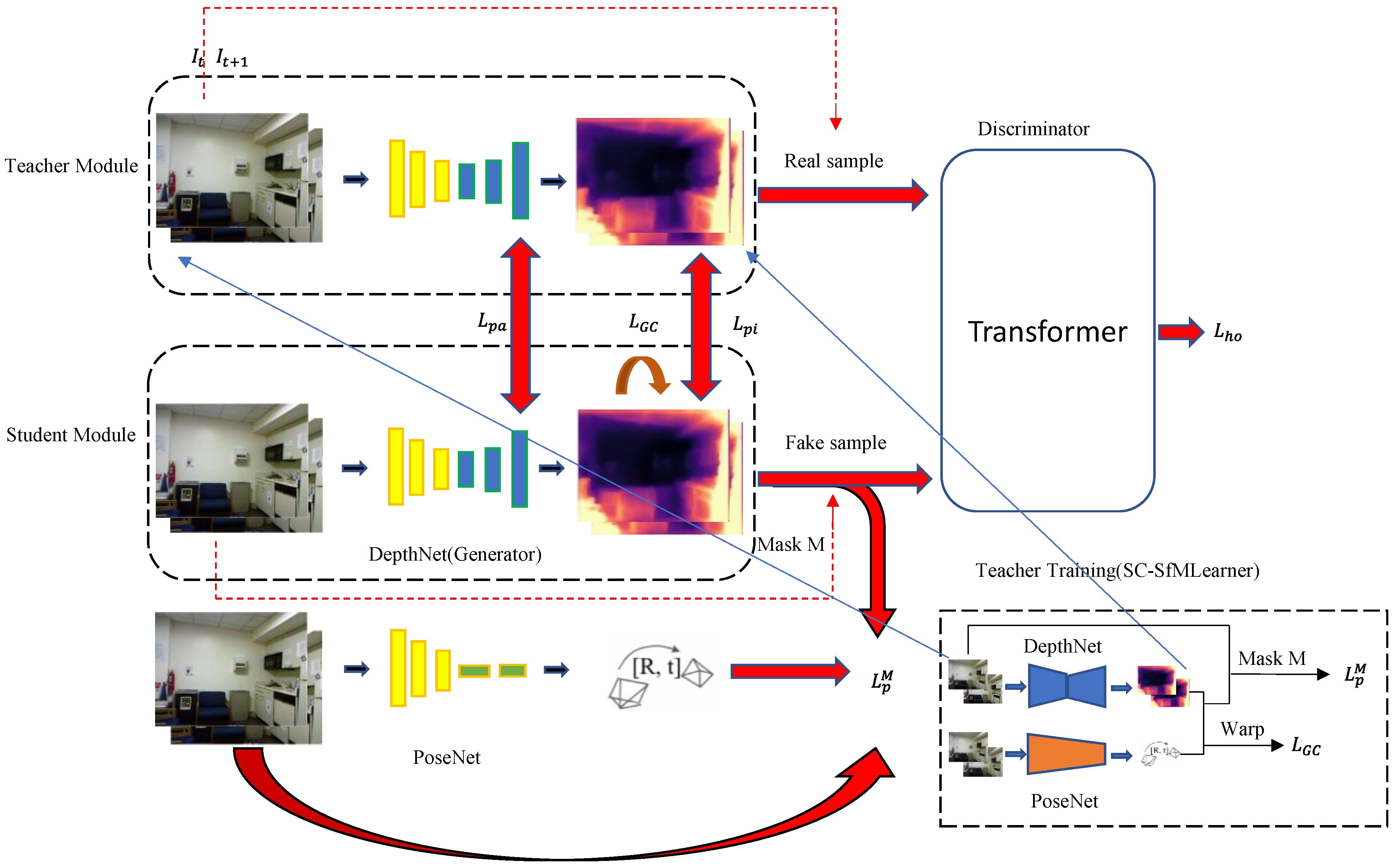
Introduce the idea of a pose network into the student network to construct photometric loss, and Transformer as the discriminator of a GAN to capture holistic information.

—

Our model achieves SOTA performance for lightweight self-supervised depth estimation models on the publicly available NYUD-V2 dataset.

—

The model size and the computational complexity of the distilled depth module only account for 22.8% and 4.8% of those from the original depth module, respectively. The inference speed of the compact network has increased by 532%.

2. Related Works

2.1. Unsupervised Depth Estimation

The core idea of unsupervised depth estimation is to reconstruct the subsequent image based on the previous image, the depth information, and pose transformation. The model is converged by minimizing the differences between the reconstructed and real images. The types of approaches can be divided into stereo pairs reconstruction and monocular sequences reconstruction. For self-supervised stereo training, Xie et al. [18] first proposed such a framework to predict discretized depth. Garg et al. [19] extended this work to continuous depth information, and Godard et al. [20] introduced left-right depth consistency to improve performance. For self-supervised monocular training, Zhou et al. [8] proposed a framework that contains a depth module and a pose module and used the photometric loss between consecutive frames as a constraint. Following this work, subsequent studies proposed further modifications to improve performance, such as different loss terms [10,21] and a better backbone [22]. Bian et al. [10] employed temporal frames depth consistency loss to force the depth consistency between consecutive frames. Yin et al. [21] and Zou et al. [23] used other flow information to encourage cross-task consistency between dense depth and optical flow. Godard et al. [9] proposed minimum reprojection loss to handle occlusions, a full-resolution multi-scale sampling method to reduce visual artifacts, and auto-masking loss to ignore pixels that violate camera motion assumptions. In view of the sharp change of depth and the difficulty of rotating pose estimation, Ji et al. [22] proposed a depth factorization module and a residual pose estimation module to address the problem.

2.2. Knowledge Distillation

The purpose of knowledge distillation [13] is to transfer knowledge from a dense model (Teacher Net) to a compact model (Student Net). This method can play an important role in the practical deployment and application of large models. It has been applied in image classification by using the class probability distribution (also known as soft targets) [13,24,25] output from the teacher network to train the student network. In this way, the relations between classes can be transferred to the compact model. In addition, Zagoruyko et al. [26] and Romero et al. [27] explored transferring related implicit information via intermediate feature maps. For the distillation of dense prediction tasks, Li et al. [28] acquired a lightweight model using a two-stage Faster-RCNN [29] in an object detection task. This work computed the difference in feature maps between the dense and compact networks at the pixel level. Xie et al. [30] aimed at semantic segmentation, with the class probabilities of each pixel and center-surrounding difference of labels of each local patch as supervision. Further, Liu et al. [15] proposed a universal strategy that can be used in all dense prediction tasks. The strategy contains pixel-wise distillation, pair-wise distillation at the structural level, and holistic distillation at the high-order cue level. This strategy is also regarded as our model’s baseline.

2.3. GAN and Transformer

GAN [31] consists of two main modules, the generator, and the discriminator. The discriminator should distinguish the real sample from the generated sample as much as possible after training, and the goal of the generator is to produce the generated sample with the smallest difference from the real sample, thereby deceiving the discriminator’s recognition ability. GANs are widely used in text generation [32,33], style transfer [34], image synthesis [31,35], etc. The idea of GAN can also be used in human pose estimation [36] and semantic segmentation [37].

Transformer [16] has drawn tremendous attention in the past few years. It uses a self-attention mechanism to replace the traditional CNN and RNN modes. In the early days, Transformer was utilized for NLP tasks [38,39,40]. Transformer’s breakthrough in the NLP field also inspired researchers in the field of computer vision. A series of models have employed Transformer to deal with CV tasks, such as ViT [41] to handle image classification, DETR [42] to deal with object detection tasks, SETR [43] to deal with semantic segmentation, and TransGAN [44] to handle adversarial training. This paper intends to employ Transformer as the discriminator module to assist model training.

3. Method

3.1. Overview

This section describes the unsupervised depth estimation distillation framework. This framework takes a single RGB image as input and produces a dense depth map. The details of our model are shown in Figure 1. In order to achieve unsupervised monocular depth prediction distillation, we follow Liu et al. [15] and propose a dense prediction distillation strategy. This strategy adopts pixel-wise similarity produced by outputs of the teacher and student networks, structured pair-wise similarity produced by intermediate feature maps, and holistic similarity produced by a CNN adversarial module, and generates an integrated loss function based on these similarities. In addition to these elements, Liu et al. [15] also employ the ground truth of related CV tasks. In this work, we abandon the ground truth module and regard the rest of the framework in [15] as our baseline model. Moreover, we introduce a pose network as an extra module to assist the convergence of the student network. Although the pose network is commonly seen in self-supervised monocular depth estimation models to produce photometric difference as supervision, no such design has been reported for the student net during distillation. Following this, the idea of GAN [15,31] is retained, and we replace the traditional CNN with Transformer [16] as the discriminator, considering its advantages in regard to global information capturing and training parallelism.

As is shown in Figure 1, our framework is composed of three main blocks: a Knowledge Distillation module, a Pose Network module, and a Transformer module. Transformer [16] is employed as the discriminator of GAN [15,31]. At the same time, the student network is regarded as the generator to produce fake samples, while the outputs of the teacher network are real samples. More detailed descriptions of these blocks are given in the following three sections.

3.2. Preliminaries

The current Knowledge Distillation Network is based on [15], which deals with dense prediction CV tasks such as semantic segmentation, object detection, and depth estimation. We adopt the ideas of pixel-wise loss, pair-wise loss, and holistic loss contained in the previous work.

Pixel-Wise Distillation. In the original paper [15], the task is semantic segmentation, which outputs the probability distribution of different classes for the teacher and student networks. The loss design in the previous paper is not suitable for estimating depth that is spatially continuous, so, in this paper, we calculate the difference between the depth maps from the teacher and student networks with the loss function defined as follows:

$$L_{pi}(S)=\frac{{\displaystyle \sum _{i\in R}{(d_i^t-d_i^s)}^2}}{W\times H}$$

(1)

where R represents all the depth map pixels, $d_i^t$ and $d_i^s$ denote the depth value of the ith pixel from the teacher network and student network, respectively, W and H denote the width and height of the depth map, respectively, and S indicates that the loss is used to update the parameters of the student module. The pixel-wise loss term is shown as $L_{pi}$ in Figure 1.

Pair-Wise Distillation. In addition to the straightforward difference between the depth maps at the pixel level, pair-wise loss is also applied in our model. This loss pays more attention to the structural similarity between intermediate feature maps produced by the teacher and student networks. In this part, two hyperparameters, i.e., connection range $\alpha$ and granularity $\beta ,$ are defined to represent the range on the maps we used to calculate the structure. Assuming the dimensions of the feature map are $W^{\prime }\times H^{\prime }\times C$, the feature map can be transformed to an affinity graph for further comparison. Each pixel on the affinity map is aggregated by $\beta$ pixels in the spatial local patch of the feature map, and we only consider structural similarity on the top-$\alpha$ close pixels, i.e., the affinity map contains $W^{\prime }\times H^{\prime }/\beta$ pixels and $\left(W^{\prime }\times H^{\prime }∕\beta \right)\times \alpha$ range connections. The aggregation method is average pooling. If we assume $f_i$ (dimension is $1\times C$) represents the ith pixel of the affinity map, $a_{ij}^t$ and $a_{ij}^s$ represent the structural similarity between the ith pixel and jth pixel of the teacher module and student module, respectively. The functions used to describe the discrepancy between the feature maps in the two modules can be defined as follows:

$$a_{ij}=\frac{f_i^T{f}_j}{({\Vert f_i\Vert }_2\times {\Vert f_j\Vert }_2)}$$

(2)

$$L_{pa}(S)=\frac{\beta }{W^{\prime }\times H^{\prime }\times \alpha }{\displaystyle \sum _{i\in R^{\prime }}{\displaystyle \sum _{j\in \alpha }{(a_{ij}^s-a_{ij}^t)}^2}}$$

(3)

where $R^{\prime }$ denotes the pixel set of the affinity graph. According to the experiment in [15], $\beta =2\times 2$ and $\alpha =W^{\prime }\times H^{\prime }/\beta$. S indicates that the loss is used to update the student module parameters. The pair-wise loss term is shown as $L_{pa}$ in Figure 1.

Holistic Distillation. Another strategy that we integrate into our framework is holistic distillation. This part can map the depth graphs generated from the teacher and student modules to high-order space and compute their holistic loss. Specifically, the original paper [15] employs a traditional self-attention CNN as a discriminator of a GAN and treats the outputs of the student and teacher net as fake and real samples, respectively. If the fake and real samples are represented as $D^s$ and $D^t$, the holistic loss function can be written as follows:

$$L_{ho}(D)=D(D^s|I)-D(D^t|I)$$

(4)

where $D(·)$ is the embedding network, i.e., the discriminator in the GAN. The depth maps $D^t$ and $D^s$ from the teacher and student networks can concatenate with the color image I and then be regarded as the inputs of the discriminator. The module is composed of two self-attention layers with four convolution blocks, and it can project the concatenated input to a high-order embedding score. D indicates that the loss is used to update the discriminator module parameters. As can be seen from the formula, the discriminator is updated to generate lower embedding scores from the compact network (student) and higher embedding scores from the dense network (teacher). In this training process, the discriminator gets smarter to distinguish fake samples from real ones. For the student net, the holistic loss can be defined as follows:

$$L_{ho}(S)=-D(D^s|I)$$

(5)

This loss can update the student module parameters by maximizing the scores generated by the discriminator. The training process contains two steps:

1.

Fix the student module parameters; minimize the $L_{ho}\left(D\right)$ to train the discriminator so that the module has enough capacity to recognize the fake and real samples.

2.

Fix the discriminator parameters; use the $L_{ho}\left(S\right)$ along with other loss terms to train the compact network, thus generating high-quality depth maps.

By iterating the above two steps, the adversarial training generates a compact module with better convergence.

The above three loss terms are regarded as our baseline.

3.3. Pose-Assisted Network

There is little research on unsupervised depth model distillation. Inspired by the previous unsupervised depth estimation networks, we integrate a pose network [8] into the student network to improve the performance of the baseline network. This module can be trained to predict the relative pose between consecutive frames and the pose information can be utilized to construct the photometric reprojection error. In our framework, it is used to assist the convergence of the student depth network and is only employed in the training stage. This module needs two consecutive frames as input, which is different from the above distillation part, where a single color image is enough. We address this problem by loading 12 images per batch, which means the batch size is 12 for the distillation part, but half for the pose module.

Just as in [8,9], $T_{t\to t^{\prime }}$ is defined as the relative pose for source image $I_{t^{\prime }}$, with respect to target image $I_t$. The reprojected image from $I_{t^{\prime }}$ can be written as follows:

$$I_{t^{\prime }\to t}=I_{t^{\prime }}\langle proj(D_t,T_{t\to t^{\prime }},K)\rangle$$

(6)

where $D_t$ is the depth map of $I_t$, K is the intrinsic parameters of the camera lens, $proj()$ denotes the resulting 2D coordinates of projected $D_t$ in $I_{t^{\prime }}$, and the angle bracket represents the sampling operator for the sake of aligning image size. With the target image $I_t$ and synthesized image $I_{t^{\prime }\to t}$, the photometric reprojection loss can be calculated as follows:

$$L_p=\frac{1}{V}{\displaystyle \sum _{p\in V}(\frac{\alpha }{2}(1-SSIM(I_t(p),I_{t^{\prime }\to t}(p)))+(1-\alpha ){\Vert I_t(p)-I_{t^{\prime }\to t}(p)\Vert }_1})$$

(7)

where $\alpha =0.85$, and $L_p$ is in the form of an L1 norm that is robust to outliers, SSIM [45] estimates the pixel-wise similarity, and V represents the valid pixels that are reprojected from $I_{t^{\prime }}$ to $I_t$ plane.

In addition, we can add another constraint between the two consecutive frames. Because of the widespread geometry inconsistency in depth estimation, we enforce the consistency of the consecutive depth maps [10] by minimizing $L_{GC}$. According to the pose information from the pose net, we can warp the source image depth to the target image plane, named $D_{t^{\prime }\to t}$. If we define depth inconsistency for each pixel p as:

$$D_{diff}(p)=\frac{\left|D_t(p)-D_{t^{\prime }\to t}(p)\right|}{D_t(p)+D_{t^{\prime }\to t}(p)}$$

(8)

Then the geometry consistency loss for each depth map can be defined as follows:

$$L_{GC}=\frac{1}{V}{\displaystyle \sum _{p\in V}{D}_{diff}(p)}$$

(9)

We use the sum of corresponding depths to normalize the depth inconsistency, thus avoiding the discrepancy in distribution. For pixels of dynamic objects and occlusions, $D_{diff}\left(p\right)$ shows an unreasonable value. Therefore, we can use a weight mask M to weigh $L_p$, thereby reducing the side effect from these pixels, i.e.,:

$$M=1-D_{diff}$$

(10)

$$L_p^M=\frac{1}{V}{\displaystyle \sum _{p\in V}(M(p)·L_p(p))}$$

(11)

Normally, edge-aware smoothness [20] can ensure that the smoothness is guided by the edge of the images. The smoothness loss is defined as follows:

$$L_s={\displaystyle \sum _p{(e^{-\nabla I_t(p)}·\nabla D_t(p))}^2}$$

(12)

where ∇ denotes the first derivative along the X and Y directions.

3.4. Transformer Adversarial Network

Recently, Transformer has been widely used in CV tasks. Jiang et al. [44] tried to utilize Transformer to construct a GAN network. As was discussed above, in this work, the holistic distillation contains the adversarial training. However, the framework used previously is a traditional CNN. For the discriminator, the holistic information must be captured to distinguish samples. Considering that Transformer can pay more attention to the global information of images, it is expected to be more suitable to acquire global cues than a traditional CNN network. Based on this assumption, we introduce Transformer as the discriminator of the adversarial training to replace the self-attention CNN module, as shown in Figure 1. We concatenate the input RGB image and depth graph to form a feature map and send this to the Transformer discriminator. The loss functions in the training are as follows:

$$L_{t-ho}(T)=T(D^s|I)-T(D^t|I)$$

(13)

and

$$L_{t-ho}(S)=-T(D^s|I)$$

(14)

where T denotes the Transformer discriminator module. Other symbols are the same as those in the holistic distillation shown in Equations (4) and (5).

3.5. Pipeline of the Current Network

The pipeline of this paper consists of a Knowledge Distillation Module, which contains pixel-wise distillation and pair-wise distillation, a Pose Assisted Module that can construct photometric loss to further improve the performance of the compact network, and a Transformer Adversarial Module that can capture global cues to converge the student network to the teacher network. The total loss function used to update the student network is as follows:

$$L(S)={\lambda }_1{L}_{pi}(S)+{\lambda }_2{L}_{pa}(S)+{\lambda }_3{L}_p^M+{\lambda }_4{L}_{GC}+{\lambda }_5{L}_s+{\lambda }_6{L}_{t-ho}(S)$$

(15)

and it consists of the loss terms from the above three modules. The hypermeters to weigh the loss terms are empirically set as ${\lambda }_1=10, {\lambda }_2=1, {\lambda }_3=1, {\lambda }_4=0.5, {\lambda }_5=0.1, \mathrm{and}{\lambda }_6=1$. $L_p^M$, $L_{GC}$, and $L_s$ are not only used in (S) because these losses also need to update the pose module parameters at the same time.

4. Experiments

The experimental work in this research contains the following three aspects:

(1)

Choosing the best student network backbone to balance prediction accuracy and computational cost. The backbone is selected from the most widely used lightweight networks;

(2)

An ablation study of our further improvements over the baseline model. We assume that the baseline performance is produced by the knowledge distillation strategy including pixel-wise, pair-wise, and holistic distillation;

(3)

The inference efficiency on medium- and low-speed computing equipment was evaluated.

4.1. Training Details

The experiments were performed on the NYUD-V2 dataset [17]. This dataset contains 464 video sequences of indoor scenes, of which, 335 scenes are used for training (302) and validation (33). We also use an officially provided dataset that contains 654 labeled images for testing. Following the pre-processing method in [46], we can reduce the rotation pose effect and change of depth range in the indoor dataset to a certain extent. Finally, 67,735 image pairs were selected for network training and we resized these images to 320 × 256. The batch size we used is 6 pairs for the pose net, i.e., 12 single images for the Knowledge Distillation Network, and the training epoch is 30. Training time is about 70 h on one 32G Nvidia Tesla V100.

In addition, we performed some experiments on traffic scenes for qualitative comparison. The dataset is from KITTI [47], which contains 11,504 images, and the images are resized to $1024\times 320$ for the convenience of training.

4.2. Selection of Teacher and Student Network

Both SC-SfMLearner [10] and Monodepth2 [9] were evaluated in this study to determine the most suitable teacher network. The relative performance of the two models is presented in

Table 1. Selection of teacher and student network.

Type	Method	Pretrain	Error ↓			Model Size (Depth)	Complexity
			AbsRel	Log10	RMS
Teacher Network	Monodepth2 [9]	√	0.156	0.066	0.561	14.84M	5.36GMac/10.7GFlops
		×	0.181	0.075	0.637
	SC-SfMLearner [10]	√	0.148	0.062	0.545	14.84M	5.36GMac/10.7GFlops
		×	0.170	0.072	0.603
Student Network	MobileNet V1 [49]	×	No Convergence			None
	MobileNet V2 [50]	√	0.169	0.071	0.589	3.62M	688.7MMac/1.35GFlops
		×	0.194	0.080	0.660
	MobileNet V3(small) [51]	√	0.163	0.068	0.581	3.38M	255.59MMac/507.26MFlops
		×	0.186	0.077	0.639
	MobileNet V3(large) [51]	√	No Convergence			6.33M	620MMac/1.21GFlops
		×	0.183	0.076	0.634
	ShuffleNet V2(0.5) [52]	√	No Convergence			4.03M	790MMac/1.55GFlops
		×	0.193	0.080	0.663
	ShuffleNet V2(1.0) [52]	√	No Convergence			5.79M	1.15GMac/2.30GFlops
		×	0.186	0.078	0.642

Note: The lowest error, parameter size, and computational complexity are marked in bold. Pretrain denotes adopting ImageNet pre-trained weights. The model size of the DepthNet includes the backbone encoder and decoder. M denotes a million parameters. Mac and Flops both denote the floating-point computation.

. It can be seen that SC-SfMLearner has a better depth performance than Monodepth2. The backbone of SC-SfMLearner is ResNet18 [48], and the parameters are updated from ImageNet pre-trained weights.

For the student network, several widely used lightweight backbones were tested on our baseline to explore the best student module, including the MobileNet series [49,50,51] and ShuffleNet series [52]. Our selection criterion is the trade-off between model size and accuracy. The experiments were performed on the baseline model by changing the backbone of the student DepthNet. The depth estimation performance was quantitatively evaluated with AbsRel, Log10, and RMS errors, as shown in Table 1. It was found that some student backbones fail to converge. MobileNet V3(small) [51] outperforms the other backbones, probably due to the fact that it combines depth-wise separable convolution in MobileNet V1 [49] and inverted residuals, and the linear bottleneck in MobileNet V2 [50], and network configuration and parameters are explored by utilizing Neural Architecture Search (NAS) [53].

The size and complexity of the converged models are also summarized in Table 1. We found that MobileNet V3 (small) [51] has the smallest model size and best accuracy, so this backbone was adopted in the current LUMDE model. If we assume that $\alpha$ denotes the parameters or computational complexity of original model M, while ${\alpha }^{*}$ denotes the parameters or computational complexity of the compressed model $M^{*}$, then we can define compression ratio R as follows:

$$R(M,M^{*})=\frac{\alpha }{{\alpha }^{*}}$$

(16)

The compression ratios of our final depth module over the teacher network are 4.4 for parameters and 21.0 for computational complexity, respectively. This means we can save 77.2% of memory space and 95.2% of computational power compared with the original network.

4.3. Ablation Study

With SC-SfMLearner as the teacher network and MobileNet V3 (small) as the optimized backbone of the student network, we first did an ablation study on the losses of baseline, i.e., pixel-wise loss, pair-wise loss, and holistic loss. The results are shown in

Table 2. Ablation study of baseline.

Losses	Error ↓			Accuracy ↑
	AbsRel	Log10	RMS	$\mathit{\delta }1$	$\mathit{\delta }2$	$\mathit{\delta }3$
L(pa)	0.333	0.128	1.007	0.506	0.777	0.903
L(pi)	0.164	0.069	0.583	0.769	0.941	0.983
L(ho)	0.306	0.121	0.955	0.525	0.799	0.918
L(pa) + L(pi)	0.163	0.069	0.583	0.769	0.941	0.983
L(pa) + L(ho)	0.321	0.123	0.978	0.522	0.789	0.909
L(pi) + L(ho)	0.163	0.069	0.582	0.768	0.941	0.983
L(pa) + L(pi) + L(ho)	0.163	0.068	0.581	0.769	0.940	0.983

. It was found that the combination of the three loss functions can generate the best performance, which is consistent with the original paper [15]. Therefore, we regard the combination of three losses as baseline and explore potential improvements on this.

We also did an ablation study on the loss functions of the PoseNet, i.e., $L_p$, $L_p^M$, $\mathrm{and} L_{GC}$. This experiment was performed in SC-SfMLearner. We did not perform an ablation assessment of the smoothness loss because many previous works [9,10,22] have validated the effectiveness of this approach and used it by default without ablation. The results are shown in

Table 3. Ablation study of PoseNet losses.

Losses	Error ↓			Accuracy ↑
	AbsRel	Log10	RMS	$\mathit{\delta }1$	$\mathit{\delta }2$	$\mathit{\delta }3$
L(P)	0.158	0.073	0.569	0.778	0.940	0.983
L(PM)	0.155	0.071	0.562	0.791	0.943	0.983
L(GC)	0.319	0.118	0.938	0.539	0.808	0.919
L(P) + L(GC)	0.155	0.065	0.559	0.796	0.943	0.982
L(PM) + L(GC)	0.148	0.062	0.545	0.803	0.948	0.985

. We find that the combination of $L_p^M$ and $L_{GC}$ is a better choice. Therefore, the following ablation study of the PoseNet module was performed upon the combination of $L_p^M$, $L_{GC}$, and $L_s$.

Moreover, we further performed an ablation study to explore potential improvements on the baseline. In the first ablation study, the PoseNet was added to the baseline to assist the convergence of the student depth network. In the second ablation study, Transformer was incorporated into the baseline to capture global image information. In the third ablation study, both PoseNet and Transformer are added into the framework to incorporate the advantages of both modules. The results are shown in

Table 4. Ablation study of different model combinations.

Method	Error ↓			Accuracy ↑
	AbsRel	Log10	RMS	$\mathit{\delta }1$	$\mathit{\delta }2$	$\mathit{\delta }3$
Teacher Network	0.148	0.062	0.545	0.803	0.948	0.985
Student Network (Baseline)	0.163	0.068	0.581	0.769	0.940	0.983
Performance	↑ 10.1%	↑ 9.7%	↑ 6.6%	↓ 4.2%	↓ 0.8%	↓ 0.2%
Baseline + PoseNet	0.160	0.067	0.575	0.775	0.942	0.984
Baseline + Transformer	0.161	0.068	0.577	0.773	0.942	0.984
Baseline + PoseNet + Transformer (LUMDE)	0.158	0.067	0.565	0.782	0.943	0.984
Performance	↑ 6.7%	↑ 8.1%	↑ 3.7%	↓ 2.6%	↓ 0.5%	↓ 0.1%

. It can be seen that the integration of PoseNet and Transformer can improve the performance of the student depth network. For baseline, the indicators increase by 10.1%, 9.7%, and 6.6% on AbsRel, Log10, and RMS errors, and decrease by 4.2%, 0.8%, and 0.2% on $\delta 1$, $\delta 2$, $\mathrm{and}\delta 3$ accuracies compared with the performance of the teacher network. For LUMDE, the indicators increase by 6.7%, 8.1%, and 3.7% on AbsRel, Log10, and RMS errors, and decrease by 2.6%, 0.5%, and 0.1% on $\delta 1$, $\delta 2$, $\mathrm{and} \delta 3$ accuracies.

It is also useful to evaluate the significance of knowledge distillation in this study. This can be achieved by investigating whether a lightweight depth model can be acquired by simply replacing the backbone of the Teacher Network (SC-SfMLearner) with the lightweight backbone used in this study. Therefore, we replaced the depth network backbone of SC-SfMLearner with MobileNet V3 (small) and trained the framework with the traditional self-supervised training method. The results are shown in

Table 5. Comparison between LUMDE and student network without KD.

Method	Error ↓
	AbsRel	Log10	RMS
Teacher Network	0.148	0.062	0.545
LUMDE	0.158	0.067	0.565
Student Network w/o KD	0.185	0.076	0.635

. Although utilizing the same pose network and training details as with SC-SfMLearner, the performance of the teacher network with a lightweight backbone is significantly worse than LUMDE. This evaluation validates the effectiveness of knowledge distillation in the current study.

The qualitative depth maps are shown in Figure 2. It can be seen that the performance of the teacher network is closest to the ground truth, which is consistent with the quantitative results in Table 4. In addition, compared with the baseline depth graphs, our optimized network (LUMDE) presents better prediction capacity on the outlines of objects, and the baseline results are somewhat hazy in some areas.

In addition, we compared our work with previous unsupervised approaches in

Table 6. Comparison with previous unsupervised work.

Type	Method	Error ↓			Accuracy ↑			Model Size (Depth)
		AbsRel	Log10	RMS	$\mathit{\delta }1$	$\mathit{\delta }2$	$\mathit{\delta }3$
w/o KD	Zhao et al. [54]	0.189	0.079	0.686	0.701	0.912	0.978	-
	Godard et al. [9]	0.160	-	0.601	0.767	0.949	0.988	14.84M
	Bian et al. [46]	0.147	0.062	0.536	0.804	0.950	0.986	14.84M
	Pan Ji et al. [22]	0.134	-	0.526	0.823	0.958	0.989	-
w/KD	Kundu et al. [14]	0.175	0.065	0.673	0.783	0.920	0.984	-
	LUMDE	0.158	0.067	0.565	0.782	0.943	0.984	3.38M

Note: w/o KD means without using knowledge distillation; w/KD means utilizing knowledge distillation.

. It can be seen in Table 6 that our model achieves SOTA results in unsupervised depth distillation with a quite low parameter size. The accuracy was also significantly increased compared with Kundu et al. [14]. In addition, the performance of LUMDE is quite competitive compared with a dense unsupervised network.

Finally, to evaluate the performance of the proposed LUMDE model on outdoor scenarios, we have also trained the model on the KITTI dataset, and made some qualitative comparisons on outdoor traffic scenes, as shown in Figure 3. It can be seen that the teacher network generates the best results. At the same time, the performance of LUMDE approaches that of the teacher net and is much better than that of the baseline network. This indicates that the proposed LUMDE model is applicable under both indoor and outdoor conditions.

4.4. Inference Efficiency

We tested our inference efficiency on both a CPU and GPU, as shown in Figure 4a,b. It can be seen that even on a CPU, our model can reach 36ms (27.8 FPS) compared with 228 ms (4.4 FPS) for the teacher net without pre- & post-processing. If we consider the pre- & post-processing, our compact network can also achieve 52 ms (19.2 FPS) on an Nvidia GeForce MX330 GPU. Pre- & post-processing refers to necessary procedures for inference such as image resizing, read & write, and coloring.

5. Conclusions

This work proposed a lightweight unsupervised monocular depth estimation network (LUMDE) achieved by knowledge distillation. The whole framework uses SC-SfMLearner as the teacher net, MobileNet V3 (small) as the backbone of the student net, and further incorporated a pose net and Transformer into the baseline distillation network to optimize the model’s performance. Experimental results show that it is possible to significantly reduce the model size and computational complexity, while still retaining SOTA accuracy. Major contributions of this paper include: (1) a suitable student backbone was selected for the compressed depth estimation network; (2) introducing a pose network and Transformer to further improve the performance of the compressed network; (3) SOTA results in self-supervised depth estimation model distillation, i.e., 0.158 on AbsRel error and 0.782 on $\delta 1$ accuracy; (4) 95.2% computational compression, 77.2% parameters compression, and real-time inference speed.

References

1. Eigen, D.; Puhrsch, C.; Fergus, R. Depth map prediction from a single image using a multi-scale deep network. Neural Info. Process. Syst. 2014, 27, 2366–2374. [Google Scholar]
2. Laina, I.; Rupprecht, C.; Belagiannis, V.; Tombari, F.; Navab, N. Deeper depth prediction with fully convolutional residual networks. In Proceedings of the 2016 Fourth International Conference on 3D Vision (3DV), Stanford, CA, USA, 25–28 October 2016; pp. 239–248. [Google Scholar]
3. Li, J.; Klein, R.; Yao, A. A two-streamed network for estimating fine-scaled depth maps from single rgb images. In Proceedings of the IEEE International Conference on Computer Vision, Venice, Italy, 22–29 October 2017; pp. 3372–3380. [Google Scholar]
4. Fu, H.; Gong, M.; Wang, C.; Batmanghelich, K.; Tao, D. Deep ordinal regression network for monocular depth estimation. In Proceedings of the IEEE Conference on Computer Vision and Pattern Recognition, Salt Lake City, GA, USA, 18–23 June 2018; pp. 2002–2011. [Google Scholar]
5. Yin, W.; Liu, Y.; Shen, C.; Yan, Y. Enforcing geometric constraints of virtual normal for depth prediction. In Proceedings of the IEEE/CVF International Conference on Computer Vision, Seoul, Republic of Korea, 27 October–2 November 2019; pp. 5684–5693. [Google Scholar]
6. Ummenhofer, B.; Zhou, H.; Uhrig, J.; Mayer, N.; Ilg, E.; Dosovitskiy, A.; Brox, T. Demon: Depth and motion network for learning monocular stereo. In Proceedings of the IEEE Conference on Computer Vision and Pattern Recognition, Honolulu, HI, USA, 21–26 July 2017; pp. 5038–5047. [Google Scholar]
7. Teed, Z.; Deng, J. Deepv2d: Video to depth with differentiable structure from motion. arXiv 2018, arXiv:1812.04605. [Google Scholar]
8. Zhou, T.; Brown, M.; Snavely, N.; Lowe, D.G. Unsupervised learning of depth and ego-motion from video. In Proceedings of the IEEE Conference on Computer Vision and Pattern Recognition, Honolulu, HI, USA, 21–26 July 2017; pp. 1851–1858. [Google Scholar]
9. Godard, C.; Mac Aodha, O.; Firman, M.; Brostow, G.J. Digging into self-supervised monocular depth estimation. In Proceedings of the IEEE/CVF International Conference on Computer Vision, Seoul, Republic of Korea, 27 October–2 November 2019; pp. 3828–3838. [Google Scholar]
10. Bian, J.; Li, Z.; Wang, N.; Zhan, H.; Shen, C.; Cheng, M.-M.; Reid, I. Unsupervised scale-consistent depth and ego-motion learning from monocular video. Neural Info. Process. Syst. 2019, 32, 35–45. [Google Scholar]
11. Han, S.; Mao, H.; Dally, W.J. Deep compression: Compressing deep neural networks with pruning, trained quantization and huffman coding. arXiv 2015, arXiv:1510.00149. [Google Scholar]
12. LeCun, Y.; Denker, J.; Solla, S. Optimal brain damage. Neural Info. Process. Syst. 1989, 2, 598–605. [Google Scholar]
13. Hinton, G.; Vinyals, O.; Dean, J. Distilling the knowledge in a neural network. arXiv 2015, arXiv:1503.02531. [Google Scholar]
14. Kundu, J.N.; Lakkakula, N.; Babu, R.V. Um-adapt: Unsupervised multi-task adaptation using adversarial cross-task distillation. In Proceedings of the IEEE/CVF International Conference on Computer Vision, Seoul, Republic of Korea, 27 October–2 November 2019; pp. 1436–1445. [Google Scholar]
15. Liu, Y.; Shu, C.; Wang, J.; Shen, C. Structured knowledge distillation for dense prediction. IEEE Trans. Pattern Anal. Mach. Intell. 2020, 6, 78–93. [Google Scholar] [CrossRef]
16. Vaswani, A.; Shazeer, N.; Parmar, N.; Uszkoreit, J.; Jones, L.; Gomez, A.N.; Kaiser, Ł.; Polosukhin, I. Attention is all you need. Neural Info. Process. Syst. 2017, 30, 214–228. [Google Scholar]
17. Silberman, N.; Hoiem, D.; Kohli, P.; Fergus, R. Indoor segmentation and support inference from rgbd images. In Proceedings of the European Conference on Computer Vision, Florence, Italy, 7–13 October 2012; pp. 746–760. [Google Scholar]
18. Xie, J.; Girshick, R.; Farhadi, A. Deep3d: Fully automatic 2d-to-3d video conversion with deep convolutional neural networks. In Proceedings of the European Conference on Computer Vision, Amsterdam, The Netherlands, 8–16 October 2016; pp. 842–857. [Google Scholar]
19. Garg, R.; Bg, V.K.; Carneiro, G.; Reid, I. Unsupervised cnn for single view depth estimation: Geometry to the rescue. In Proceedings of the European Conference on Computer Vision, Amsterdam, The Netherlands, 8–16 October 2016; pp. 740–756. [Google Scholar]
20. Godard, C.; Mac Aodha, O.; Brostow, G.J. Unsupervised monocular depth estimation with left-right consistency. In Proceedings of the IEEE Conference on Computer Vision and Pattern Recognition, Honolulu, HI, USA, 21–26 July 2017; pp. 270–279. [Google Scholar]
21. Yin, Z.; Shi, J. Geonet: Unsupervised learning of dense depth, optical flow and camera pose. In Proceedings of the IEEE Conference on Computer Vision and Pattern Recognition, Salt Lake City, GA, USA, 18–23 June 2018; pp. 1983–1992. [Google Scholar]
22. Ji, P.; Li, R.; Bhanu, B.; Xu, Y. Monoindoor: Towards good practice of self-supervised monocular depth estimation for indoor environments. In Proceedings of the IEEE/CVF International Conference on Computer Vision, Montreal, QC, Canada, 11–18 October 2021; pp. 12787–12796. [Google Scholar]
23. Zou, Y.; Luo, Z.; Huang, J.-B. Df-net: Unsupervised joint learning of depth and flow using cross-task consistency. In Proceedings of the European Conference on Computer Vision (ECCV), Munich, Germany, 8–14 September 2018; pp. 36–53. [Google Scholar]
24. Ba, J.; Caruana, R. Do deep nets really need to be deep? Neural Info. Process. Syst. 2014, 27, 2654–2662. [Google Scholar]
25. Urban, G.; Geras, K.; Kahou, S.; Aslan, O.; Wang, S.; Caruana, R.; Mohamed, A.; Philipose, M.; Richardson, M. Do Deep Convolutional Nets Really Need to be Deep (Or Even Convolutional)? arXiv 2016, arXiv:1603.05691. [Google Scholar]
26. Zagoruyko, S.; Komodakis, N. Paying more attention to attention: Improving the performance of convolutional neural networks via attention transfer. arXiv 2016, arXiv:1612.03928. [Google Scholar]
27. Romero, A.; Ballas, N.; Kahou, S.E.; Chassang, A.; Gatta, C.; Bengio, Y. Fitnets: Hints for thin deep nets. arXiv 2014, arXiv:1412.6550. [Google Scholar]
28. Li, Q.; Jin, S.; Yan, J. Mimicking very efficient network for object detection. In Proceedings of the IEEE Conference on Computer Vision and Pattern Recognition, Honolulu, HI, USA, 21–26 July 2017; pp. 6356–6364. [Google Scholar]
29. Ren, S.; He, K.; Girshick, R.; Sun, J. Faster r-cnn: Towards real-time object detection with region proposal networks. Neural Info. Process. Syst. 2015, 28, 91–99. [Google Scholar] [CrossRef] [PubMed] [Green Version]
30. Xie, J.; Shuai, B.; Hu, J.-F.; Lin, J.; Zheng, W.-S. Improving fast segmentation with teacher-student learning. arXiv 2018, arXiv:1810.08476. [Google Scholar]
31. Goodfellow, I.; Pouget-Abadie, J.; Mirza, M.; Xu, B.; Warde-Farley, D.; Ozair, S.; Courville, A.; Bengio, Y. Generative adversarial nets. Neural Info. Process. Syst. 2014, 27, 139–144. [Google Scholar]
32. Wang, H.; Qin, Z.; Wan, T. Text generation based on generative adversarial nets with latent variables. In Proceedings of the Pacific-Asia Conference on Knowledge Discovery and Data Mining, Melbourne, Australia, 3–6 June 2018; pp. 92–103. [Google Scholar]
33. Yu, L.; Zhang, W.; Wang, J.; Yu, Y. Seqgan: Sequence generative adversarial nets with policy gradient. In Proceedings of the AAAI Conference on Artificial Intelligence, San Francisco, CA, USA, 4–9 February 2017. [Google Scholar]
34. Johnson, J.; Alahi, A.; Fei-Fei, L. Perceptual losses for real-time style transfer and super-resolution. In Proceedings of the European Conference on Computer Vision, Amsterdam, The Netherlands, 8–16 October 2016; pp. 694–711. [Google Scholar]
35. Karras, T.; Aila, T.; Laine, S.; Lehtinen, J. Progressive Growing of GANs for Improved Quality, Stability, and Variation. In Proceedings of the ICLR, Vancouver, BC, Canada, 30 April–3 May 2018. [Google Scholar]
36. Chen, Y.; Shen, C.; Wei, X.-S.; Liu, L.; Yang, J. Adversarial posenet: A structure-aware convolutional network for human pose estimation. In Proceedings of the IEEE International Conference on Computer Vision, Venice, Italy, 22–29 October 2017; pp. 1212–1221. [Google Scholar]
37. Luc, P.; Couprie, C.; Chintala, S.; Verbeek, J. Semantic segmentation using adversarial networks. arXiv 2016, arXiv:1611.08408. [Google Scholar]
38. Devlin, J.; Chang, M.-W.; Lee, K.; Toutanova, K. Bert: Pre-training of deep bidirectional transformers for language understanding. arXiv 2018, arXiv:1810.04805. [Google Scholar]
39. Radford, A.; Narasimhan, K.; Salimans, T.; Sutskever, I. Improving Language Understanding by Generative Pre-Training. Available online: https://www.cs.ubc.ca/~amuham01/LING530/papers/radford2018improving.pdf (accessed on 12 June 2018).
40. Brown, T.; Mann, B.; Ryder, N.; Subbiah, M.; Kaplan, J.D.; Dhariwal, P.; Neelakantan, A.; Shyam, P.; Sastry, G.; Askell, A. Language models are few-shot learners. Neural Info. Process. Syst. 2020, 33, 1877–1901. [Google Scholar]
41. Dosovitskiy, A.; Beyer, L.; Kolesnikov, A.; Weissenborn, D.; Zhai, X.; Unterthiner, T.; Dehghani, M.; Minderer, M.; Heigold, G.; Gelly, S. An image is worth 16x16 words: Transformers for image recognition at scale. arXiv 2020, arXiv:2010.11929. [Google Scholar]
42. Carion, N.; Massa, F.; Synnaeve, G.; Usunier, N.; Kirillov, A.; Zagoruyko, S. End-to-end object detection with transformers. In Proceedings of the European Conference on Computer Vision, Online, 23–28 August 2020; pp. 213–229. [Google Scholar]
43. Zheng, S.; Lu, J.; Zhao, H.; Zhu, X.; Luo, Z.; Wang, Y.; Fu, Y.; Feng, J.; Xiang, T.; Torr, P.H. Rethinking semantic segmentation from a sequence-to-sequence perspective with transformers. In Proceedings of the IEEE/CVF Conference on Computer Vision and Pattern Recognition, Online, 19–25 June 2021; pp. 6881–6890. [Google Scholar]
44. Jiang, Y.; Chang, S.; Wang, Z. Transgan: Two pure transformers can make one strong gan, and that can scale up. Neural Info. Process. Syst. 2021, 34, 14745–14758. [Google Scholar]
45. Wang, Z.; Bovik, A.C.; Sheikh, H.R.; Simoncelli, E.P. Image quality assessment: From error visibility to structural similarity. IEEE Trans. Image Process. 2004, 13, 600–612. [Google Scholar] [CrossRef] [PubMed]
46. Bian, J.-W.; Zhan, H.; Wang, N.; Chin, T.-J.; Shen, C.; Reid, I. Unsupervised depth learning in challenging indoor video: Weak rectification to rescue. arXiv 2020, arXiv:2006.02708. [Google Scholar]
47. Geiger, A.; Lenz, P.; Urtasun, R. Are we ready for autonomous driving? The kitti vision benchmark suite. In Proceedings of the 2012 IEEE Conference on Computer Vision and PATTERN recognition, Providence, RI, USA, 16–21 June 2012; pp. 3354–3361. [Google Scholar]
48. He, K.; Zhang, X.; Ren, S.; Sun, J. Deep residual learning for image recognition. In Proceedings of the IEEE Conference on Computer Vision and Pattern Recognition, Las Vegas, NEV, USA, 27–30 June 2016; pp. 770–778. [Google Scholar]
49. Howard, A.G.; Zhu, M.; Chen, B.; Kalenichenko, D.; Wang, W.; Weyand, T.; Andreetto, M.; Adam, H. Mobilenets: Efficient convolutional neural networks for mobile vision applications. arXiv 2017, arXiv:1704.04861. [Google Scholar]
50. Sandler, M.; Howard, A.; Zhu, M.; Zhmoginov, A.; Chen, L.-C. Mobilenetv2: Inverted residuals and linear bottlenecks. In Proceedings of the IEEE Conference on Computer Vision and Pattern Recognition, Salt Lake City, GA, USA, 18–23 June 2018; pp. 4510–4520. [Google Scholar]
51. Howard, A.; Sandler, M.; Chu, G.; Chen, L.-C.; Chen, B.; Tan, M.; Wang, W.; Zhu, Y.; Pang, R.; Vasudevan, V. Searching for mobilenetv3. In Proceedings of the IEEE/CVF International Conference on Computer Vision, Seoul, Republic of Korea, 27 October–2 November 2019; pp. 1314–1324. [Google Scholar]
52. Ma, N.; Zhang, X.; Zheng, H.-T.; Sun, J. Shufflenet v2: Practical guidelines for efficient cnn architecture design. In Proceedings of the European Conference on Computer Vision (ECCV), Munich, Germany, 8–14 September 2018; pp. 116–131. [Google Scholar]
53. Zoph, B.; Le, Q.V. Neural architecture search with reinforcement learning. arXiv 2016, arXiv:1611.01578. [Google Scholar]
54. Zhao, W.; Liu, S.; Shu, Y.; Liu, Y.-J. Towards better generalization: Joint depth-pose learning without posenet. In Proceedings of the IEEE/CVF Conference on Computer Vision and Pattern Recognition, Seattle, IL, USA, 16–20 June 2020; pp. 9151–9161. [Google Scholar]
Figure 1. Overview of the LUMDE architecture. Baseline results are generated by the knowledge distillation module with pixel-wise loss, pair-wise loss, and holistic loss (CNN discriminator). PoseNet is further incorporated into the student network to improve model performance during training, and Transformer is adopted to replace CNN as the discriminator in the GAN.
Applsci 12 12593 g001
Figure 2. Qualitative comparison of depth ground truth, depth from teacher network, baseline, and LUMDE of indoor scenes, with RGB images shown in the first column.
Applsci 12 12593 g002
Figure 3. Qualitative comparison of depth ground truth, depth from teacher network, baseline, and LUMDE about outdoor traffic scenes, with RGB images shown in the first column.
Applsci 12 12593 g003
Figure 4. (a) Inference efficiency on an i5 core CPU; (b) Inference efficiency on an Nvidia GeForce MX330 GPU. In the inference stage, only the DepthNet is used to test inference efficiency. Pre- & post-processing refer to the necessary procedures for inference such as image resizing, read & write, and coloring. Image size is 640 × 320.
Applsci 12 12593 g004