
3D Convolution Recurrent Neural Networks for Multi-Label Earthquake Magnitude Classification †


1
Department of Systems and Control Engineering, School of Engineering, Tokyo Institute of Technology, 2-12-1 Ookayama, Meguro-ku, Tokyo 152-8552, Japan
2
Honda Research Institute Japan Co., Ltd., 8-1, Honcho, Wako 351-0188, Japan
*
Author to whom correspondence should be addressed.
†
This paper is an extended version of our paper published in IEEE/SICE International Symposium on System Integration, “EMC: Earthquake Magnitudes Classification on Seismic Signals via Convolutional Recurrent Networks”.
Appl. Sci. 2022, 12(4), 2195; https://doi.org/10.3390/app12042195
Submission received: 25 January 2022
/
Revised: 15 February 2022
/
Accepted: 18 February 2022
/
Published: 20 February 2022
(This article belongs to the Special Issue Application of Artificial Intelligence in Signal Processing)
Abstract
:We examine a classification task in which signals of naturally occurring earthquakes are categorized ranging from minor to major, based on their magnitude. Generalized to a single-label classification task, most prior investigations have focused on assessing whether an earthquake’s magnitude falls into the minor or large categories. This procedure is often not practical since the tremor it generates has a wide range of variation in the neighboring regions based on the distance, depth, type of surface, and several other factors. We present an integrated 3-dimensional convolutional recurrent neural network (3D-CNN-RNN) trained to classify the seismic waveforms into multiple categories based on the problem formulation. Recent studies demonstrate using artificial intelligence-based techniques in earthquake detection and location estimation tasks with progress in collecting seismic data. However, less work has been performed in classifying the seismic signals into single or multiple categories. We leverage the use of a benchmark dataset comprising of earthquake waveforms having different magnitude and present 3D-CNN-RNN, a highly scalable neural network for multi-label classification problems. End-to-end learning has become a conventional approach in audio and image-related classification studies. However, for seismic signals classification, it has yet to be established. In this study, we propose to deploy the trained model on personal seismometers to effectively categorize earthquakes and increase the response time by leveraging the data-centric approaches. For this purpose, firstly, we transform the existing benchmark dataset into a series of multi-label examples. Secondly, we develop a novel 3D-CNN-RNN model for multi-label seismic event classification. Finally, we validate and evaluate the learned model with unseen seismic waveforms instances and report whether a specific event is associated with a particular class or not. Experimental results demonstrate the superiority and effectiveness of the proposed approach on unseen data using the multi-label classifier.
1. Introduction
The recent advances in machine learning have been highly influential in classification-related tasks where the input sensor data is audio or image. Categorizing multiple labels is an essential and well-studied topic [1,2,3,4] with computer vision [5,6,7,8,9], audio classification [10,11], natural language processing [12,13], and information retrieval [14] applications. However, no classifiers are available in seismic signal processing literature to perform multi-label classification on earthquake categorization tasks. The typical classification application for seismic data is to distinguish between earthquakes buried in the seismic noise. Although the earthquake detection problem has been addressed differently, most of these methods are proposed as binary classification (e.g., [15,16,17]). These works referred to earthquake recognition as a single-label task: determining whether a seismic signal belongs to an earthquake or a seismic noise.
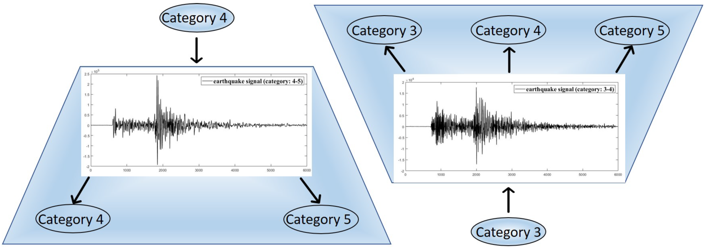
Nevertheless, it is often not natural to assume earthquake detection as a binary classification task. There are primarily two explanations for this inappropriateness. To begin, the limitation of addressing earthquake detection as a binary classification task is incompleteness; a single earthquake label may not accurately describe the earthquake category for a particular seismic wave. For example, it will be a subjective value, but it can represent a human impression of the earthquake better than the physical value of magnitude. Secondly, it also demonstrates uncertainty, i.e., the class boundaries among many earthquake categories are ambiguous essentially. We see from many reported earthquakes worldwide; the series of effects from an earthquake depends on the shallowness and duration of an earthquake and its magnitude. Sometimes, two earthquakes slightly differ between their magnitudes but demonstrate the same effect on the ground. When referring to an intermediate earthquake condition, it is difficult to identify whether the earthquake category is “minor” or “slightly major” in terms of its effect on the ground. Currently, available earthquake datasets do not provide information about the intensity or felt reports. For this reason, we have converted the multiclass problem to a multi-label problem where each earthquake waveform can have multiple categories simultaneously, i.e., for example, when an earthquake happens, it has one value generally known as the magnitude that describes the size. However, we can have many intensity values distributed around the epic center and located in different geographic areas for this particular earthquake. We propose, by using regression analysis, the earthquake magnitudes can be modeled into multiple classes, i.e., after dataset conversion, an earthquake of magnitude “1” can belong to class “0”, “1” or “2” simultaneously, which in this particular study is considered as a multilabel classification problem (see Figure 1). Although the labels can be interpreted as intensities, however, they are not the actual intensities measured by the instrument. To avoid ambiguity, we do not label them as intensities. This study only uses the magnitude information from which we convert the single label information to multi-label information. The uncertainty associated with these border seismic signals makes it impossible to distinguish earthquakes even from a human viewpoint, and no prior study has addressed this issue.
Moreover, many researchers [18] find ways to employ low-cost ground motion sensors in cities to monitor seismic activity in urban areas. The primary motivation to conduct this study is to pave the way for data-centric approaches and deploy an efficiently trained deep learning model on personal seismometers where seismic noise is high. We believe that using deep learning models on these sensors to categorize earthquake severity in an urban environment will significantly increase the response time.
Furthermore, categorizing earthquakes into multiple classes is a time-consuming operation in a classical method. For example, in classifying the earthquake into several categories, the earthquake magnitude must be estimated using the following steps: firstly, we compute the sensor response; secondly, we convolve the estimated response with a signal response from a Wood Anderson instrument (specialized to measure the signal response accurately) [19], thirdly, transform the original signal counts to acceleration. Moreover, to estimate the correct earthquake magnitude, we need to apply the attenuation models for each region and introduce some correction terms. Finally, we average the measurements from multiple nearby single stations to accurately estimate the earthquake magnitude.
Motivated by the reasons mentioned above, we propose to view earthquake magnitude categorization as a multi-label classification task, assigning several labels to a seismic signal based on its reported magnitude by a seismograph. We propose to solve this task using a 3-dimensional convolutional recurrent architecture (3D-CNN-RNN). Encouraged by the significant advancements in convolutional neural networks (CNN) [20,21,22,23,24,25], we utilize CNN as the earthquake feature extractor. On the other hand, numerous earthquake classes demonstrate high co-occurrence correlations in seismic data. For example, earthquakes having magnitude 1.5–2.5 can exhibit the same seismic pattern and have similar effects, while magnitudes 1.5 and 4.5 can never have indistinguishable fallout. With the recent success of recurrent neural networks (RNN) [26,27,28] in modeling the dependencies, we propose to employ separate RNNs on each kernel of the last convolutional layer to model the dependencies among labels and predict earthquake categories step by step. In this way, the network can implicitly integrate the information inferred using the previous hidden states when recognizing the subsequent labels.
Due to the acoustic nature of the seismic signal, it exhibits similar properties as an audio signal; therefore, we propose to extract log-Mel features for algorithm training. The signal is easily convertible to a log-Mel spectrogram and is treated as an input to the CNN. Moreover, it is imperative to make the earthquake signal discriminative and preserve the spatial information of the spectrogram. For this purpose, recurrent layers are employed on each kernel of the third CNN layer to leverage additional spectral information for the earthquake recognition task. In this study, CNN is used for local feature extraction and recurrent layers to model the state-to-state and input-to-state transformations, capturing information in the spatiotemporal domain.
In addition, considering that there is no dataset for the multi-label earthquake recognition task, we propose constructing a new dataset in this study. The data catalog comprises 93 K seismic waveforms, out of which six new classes are generated from two categories of an existing earthquake dataset, STEAD (STanford EArthquake Dataset) [29]. In summary, we claim three main contributions of this work:
- We examine earthquake magnitude categorization as a multi-label classification task by evaluating the features extracted through log-Mel spectrograms and analyzing the relationships among different earthquake classes.
- We present a 3D-CNN-RNN based architecture to evaluate the multi-label earthquake classification task. It encapsulates a 3D-CNN to extract features from an input spectrogram, and recurrent layers are employed on each kernel of the final CNN layer to model the similarities among different earthquake signals.
- We develop a new multi-label earthquake dataset and reorganize an existing dataset [29] for the earthquake categorization task.
This paper is organized as follows: Section 2 discusses our approach to categorize the earthquake magnitudes and comprehensively explains the use of 3D convolutional and recurrent neural networks and their adaptation to multi-label earthquake magnitudes classification tasks. Section 3 describes the dataset properties, extraction, and transformation methods to evaluate the proposed framework. Section 4 describes the feature extraction methods, and Section 5 explains our experiments on the transformed dataset acquired from STEAD. Section 6 concludes this work and discusses possible future research directions motivated by the proposed method.
2. Our Approach
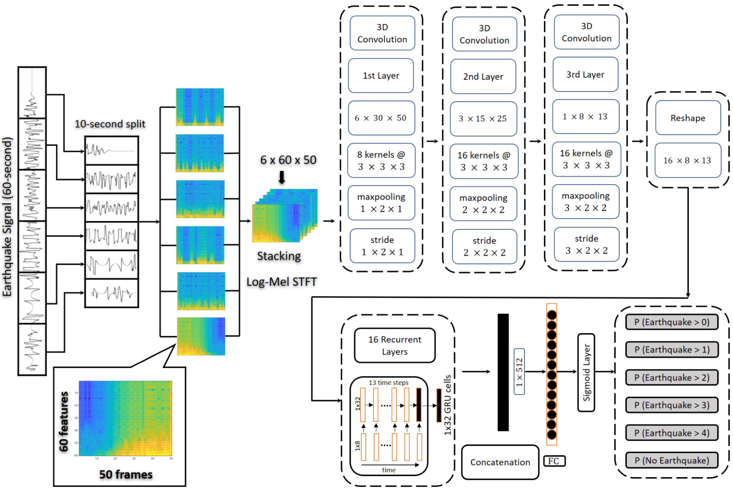
In this work, to comprehensively categorize the earthquake magnitudes, we propose to treat earthquake magnitudes categorization as a multi-label classification task. Moreover, a 3D-CNN-RNN incorporating recurrent layers is constructed to undergo this task, which simultaneously frames and classifies earthquake magnitudes, allowing multiple labels to belong to a single earthquake category. To attain higher dimensionality in the temporal and spatial domain, we convert the raw seismic signals into log-Mel-based spectrograms, feed the extracted features to a 3D-CNN-RNN architecture and perform multi-label classification predictions. The complete architecture of our proposed method is presented in Figure 2. The network comprises three parts, i.e., feature engineering, the 3D-CNN, and recurrent layers assimilated with convolutional layers. The feature engineering part extracts the log-energies in the Mel scale and creates a log-Mel spectrogram. The convolution layers extract the spatial information, while recurrent layers capture the temporal features from seismic waveforms.
2.1. 3D Convolutional Neural Networks
Deep neural networks, like CNN, have shown significant performance in a variety of applications, including audio and image. However, it has not been examined for the multi-label earthquake classification task. A CNN comprises layers with filters, frequently referred to as kernels, seeking specific characteristics in the earthquake signals. 3D-CNN [30], having the above filters represented in a three-dimensional matrix, extract spatial and temporal information and identify patterns in the input. During periods of intense seismic activity, it is highly probable that the changing behavior of the signal is likely to be understood in the temporal domain, which inspired us to implement 3D-CNN by convolving a kernel having three dimensions. We produce these convolutions in this work by stacking numerous neighboring spectrograms of a 60-second ground motion divided into a 10-s frame. In a conventional setting of convolutional layer, operations are carried out in three stages: firstly, we perform convolution operation using 3D kernels to create matrix transformations linearly; secondly, each linear matrix convolution passes through spatial and temporal features in the spectrogram by employing a non-linear activation (ReLU) function; and finally, the feature maps are downsampled using a pooling operation. Various combinations of these essential basic components may be used to create the CNN.
The value of any element at position in the jth feature space of the ith layer is represented by , and defined as,
where g is the activation function, is a bias for the feature space, is the size of the 3-dimensional filter along the time axis, is the th value of the filter associated to mth feature in the former layer.
2.2. Recurrent Neural Network (RNN)
In sequence-to-sequence learning, RNNs are a subset of neural networks that can untangle irregular input features by utilizing their primary internal memory and process-changing sequences through recurrent layers. RNNs can unfold sequence-to-sequence learning tasks as they retain temporal features across their inputs, making them optimal for time-domain-related tasks. Numerous practical applications [28] propose employing ‘gatedrecurrent units’, also known as GRUs, since they overcome the issue of vanishing gradients that might occur while training neural networks. Due to the lack of an output gate, GRUs have fewer network parameters and are thus more viable for practical implementation than LSTM-based recurrent networks. GRUs operate based on a single gating unit and can concurrently update the gated units in a recurrent structure. Moreover, GRUs train faster, are computationally more efficient and have comparable performance to LSTMs on less training data [17,31]. Furthermore, the model is intended to be deployed in real-time in the future, and GRUs having fewer parameters than LSTMs make it an ideal candidate for the magnitude classification task. Following are the equations for updating gated recurrent unit [18] states:
where u stands for the update gate and r for the “reset” gate. Their value is separately defined as:
In gated recurrent units, portions of the state vector are “ignored” independently using update and reset gates, allowing the temporal information and forget-states of distinct units to be controlled dynamically.
2.3. 3-Dimensional Convolutional Recurrent Architecture
This section describes a 3D-CNN-RNN architecture for classifying earthquake magnitudes. In literature, there are numerous combinations of CNN-RNN topologies to choose from; we would want to focus on the core of 3D-CNN, which is three convolutional layers. In addition, we also incorporate RNN layers into all the kernels of the third convolutional layer. Moreover, we extract information using a fully connected (FC) last layer to identify earthquake magnitudes and perform the classification task. We process features based on log-Mel spectrograms and provide the extracted features to the 3D-CNN. After applying 3D kernels succeeded by a max-pooling operation, as shown in Figure 2, the CNN is designed using three convolutional layers as a preliminary step. With the 3D filter, we create a receptive field of in size. We further extract the feature maps using a kernel to fetch the features in the spatial dimension, whereas the third dimension scans it along the time axis. Each convolutional layer has a max-pooling operation of for the first, for the second, and for the third.
Stride, padding, and filter size are three of the most often used hyper-parameters for creating convolutional computations, and we choose the most optimal parameters for this study. The stride parameter specifies the size of the step taken by the receptive field each time. We downsample the inputs along each dimension while gradually extending the dynamic range using the max-pooling procedure. For each convolutional layer, a rectified linear unit is used as an activation function, where represents the maximum value for an activation function. Rectified linear unit’s (ReLU’s) back-propagation rule removes any gradient components smaller than zero. Finally, batch normalization is performed to each convolutional layer to optimize the learning rate. We prevent overfitting by using a dropout rate of 0.3 in each convolutional layer. Weights are randomly initialized for the training phase using Xavier initialization [32]. The final convolutional layer has 16 filters; therefore, GRUs are used on each filter to keep the temporal information, yielding 16 GRUs. We downsample the log-Mel spectrograms from 50 temporal features to 13, creating a recurrent layer for each feature map. Finally, recurrent layers are concatenated and linked to the FC layer using a many-to-one architecture. In addition, we obtain a flattened tensor from the previously concealed hidden layer. With the help of the sigmoid layer, it transforms them into the required output and generates a 6-dimensional vector that represents the earthquake categories.
3. Data and Methods
To the best of our knowledge, no prior datasets have been used to study earthquake magnitude categorization as a multi-label classification task. Therefore, to assess the proposed framework, we extract the dataset presented in [29] and further transform the data as utilized in [17]. In this section, we first introduce the properties and then the transformation procedure of the dataset.
3.1. Properties of Dataset
A worldwide earthquake database was published recently, encompassing 1.2 million seismic waveforms obtained from different major networks globally. The data comprises earthquakes that occurred between January 1984 and August 2018. The data catalog is named STEAD, and it was recently made opensource to expedite research in this area. The data is split up into two subsets: local quakes and seismological noise. Typically, earthquakes are monitored, and their position is estimated using measurements from seismometers acquired in east-west, north-south, and vertical directions. Generally, the seismic waveforms often contain different lengths of pre-event data before the primary wave (P-wave); however, the seismic waveforms in the given dataset [29] are well aligned and do not affect the feature extraction process. Nearly 1,050,000 three-component seismological events are included in the database. Each one-minute-long waveform comprises 6000 samples of seismic activity. We extract the vertical component from the Stanford database for the presented work as the model is intended to be installed on an inexpensive personal seismometer equipped with a vertical component sensor designed to detect ground motion in an urban region with strong seismic noise.
Each waveform in the presented dataset comprises 32 properties, making it suitable for multi-class and multi-label-related research. A major part of the database consists of earthquake waveforms with a magnitude of <2.5 (on the Richter scale), which is indicated as an attribute named ‘source magnitude’. To perform this research, we filter the recorded waveforms into several classes by utilizing the features as explained in STEAD. The Stanford database has distinctive waveforms: ones recognized automatically by algorithms and, secondly, manually picked by seismic stations. These are referred to as ‘automatic’ and ‘manual’ picks. We examined the signals recorded by seismographs to train the algorithms, i.e., ‘manual’ selections. Training and testing sets have distinct waveforms with no overlapping signals. The ‘source magnitude’ and ‘earthquakes’ attributes are used to distinguish waveforms and are separated into several categories. We ensure consistency by detrending (i.e., mean shifted) the data, using a band-passed filter from 1–45 Hz, and resampling the signals at 100 Hz. We built our dataset from the Stanford earthquake database using the characteristics indicated above. Our experiment used 93,144 waveforms, 65,208 for learning the model, and 27,936 for testing. The training and test sets are composed of 70% and 30%, respectively. We defined five classes of earthquakes and constructed the dataset necessary to conduct multi-class classification. Additionally, we labeled the signals with the numerical values ‘(0–1)’, ‘(1–2)’, ‘(2–3)’, ‘(3–4)’, ‘(4–8)’, and ‘Non-earthquake’, where ‘(0–1)’ means we include all the earthquakes with magnitude greater than zero and less than equal to one in this category. The same procedure is valid for all the other categories. The complete distribution of earthquake categories and accompanying training and test sets are shown in Table 1.
3.2. Transforming Multi-Class to Multi-Label Dataset
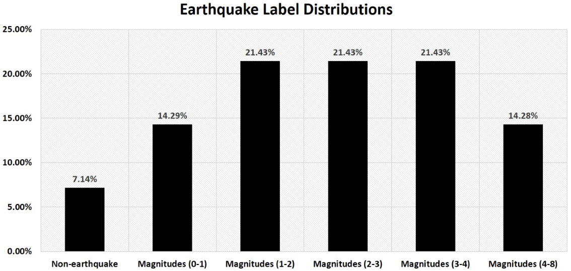
This study takes a different approach and transforms a multi-classification task into a multi-label task. The simplest example of a transformation of this type is to use regression. We receive multiple probabilities for each class using an algorithm trained on multi-class classification tasks as presented in [33]. We convert the target labels by using a probability threshold value of 0.5. It assigns a numeric value of 1 if the predicted class misclassifies with a threshold value greater than 0.5, whereas it assigns a numeric value of 0 otherwise. Because we employ a regressor, predicting a specific instance may not result in a value of exactly 0 or 1 for each target. For this reason, we propose thresholding to transform the dataset into a multi-label problem where each earthquake waveform can belong to multiple categories simultaneously. The detailed label distributions of earthquake magnitudes associated with the multi-label dataset are presented in Figure 3.
4. Experiments
Data Representation: Feature Extraction
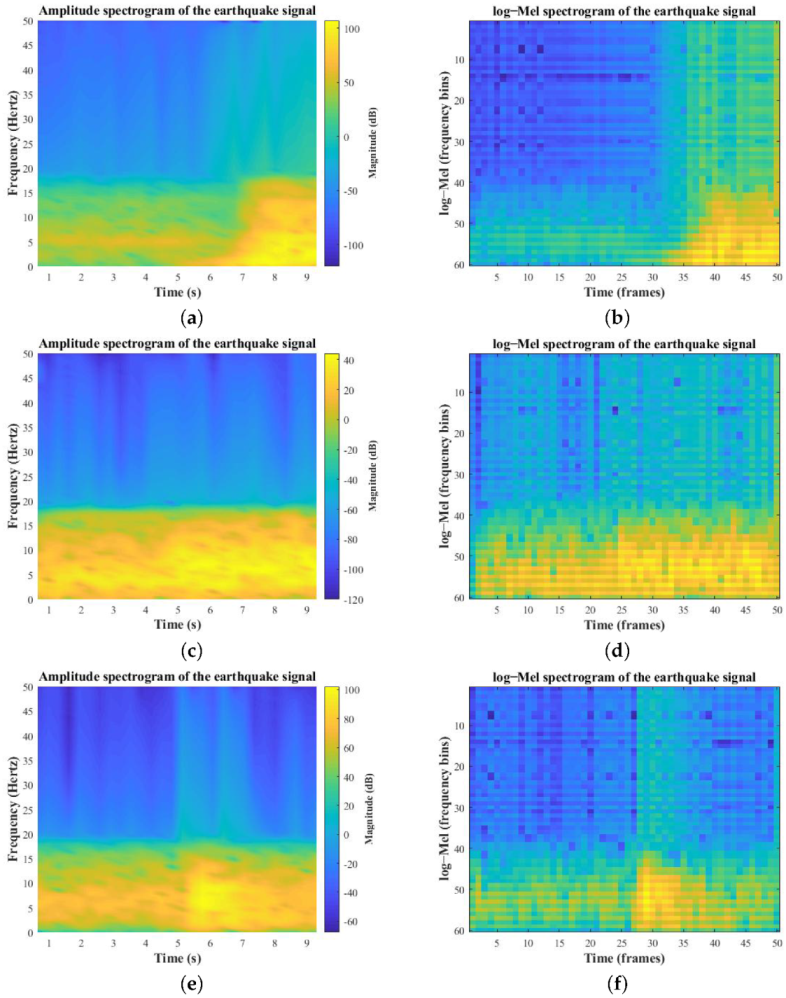
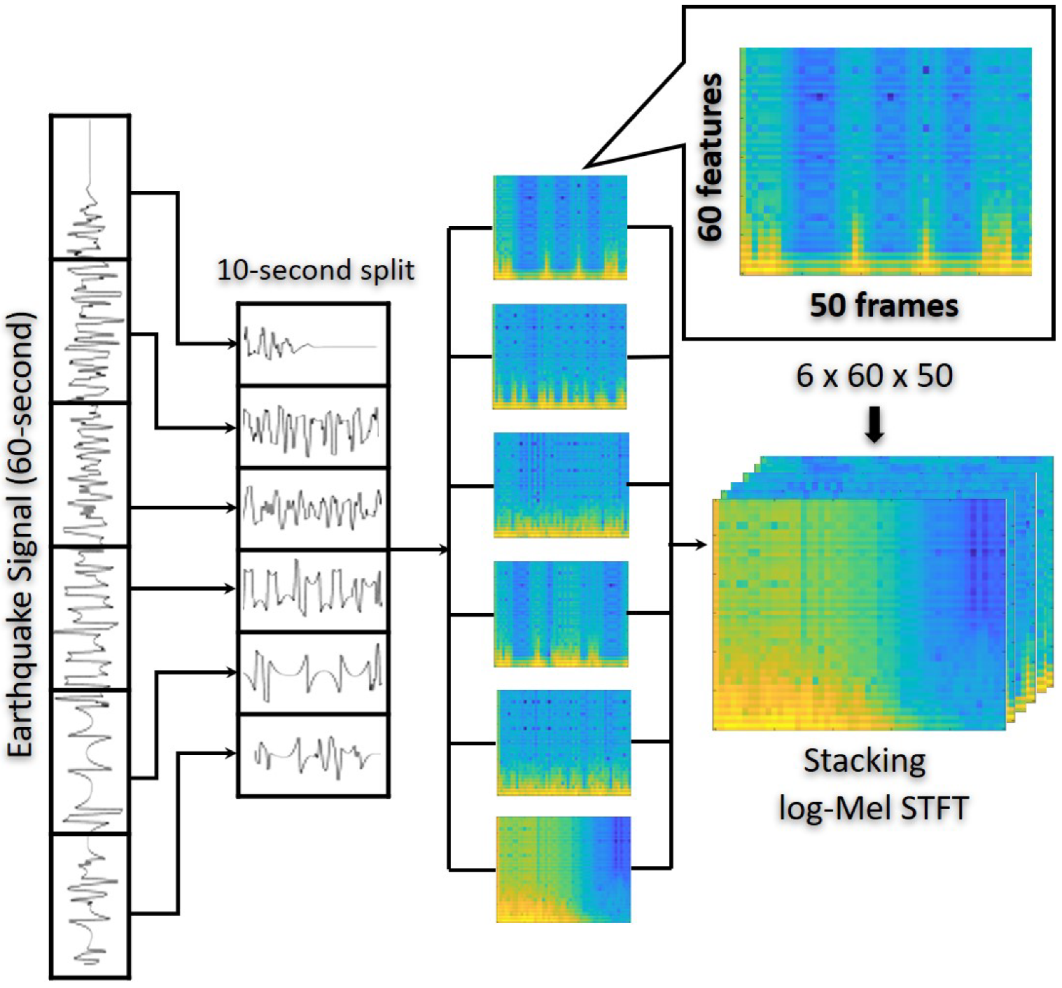
Here, we propose interpreting log-energies in the Mel scale at the frame level to represent earthquake signals accurately. Log-Mel spectrograms are constructed by linearly spacing triangular-shape filters in the Mel scale. The extraction of log-energies is identical to those of MFCCs [34], except that the extraction of discrete-continuous Transform (DCT) is eliminated while calculating the log-Mel energies. Log-Mel was initially proposed as a speech feature with a log scale filter and gives an impression that extra non-seismic wave components are covered. However, in this work, we need to discriminate seismic waves from a mixture of many types of sources, including various frequencies. Moreover, extracting features from seismic data using the log-Mel scaling help retain maximum spatial components while simultaneously keeping the temporal features. Firstly, 1-min collected waveforms are split into six ten-second chunks. Secondly, each 10-s sample is processed using triangular-shaped filters to produce a single log-Mel time-frequency spectrogram. A 10-s sample is sent through a sequence of 400 ms window signals, which results in 49 windows. However, we have added a zero at the end of the signal to obtain 50 frames to maintain consistency. A 10-s sample contains 1000 samples, but after adding ‘0’ at the end, it makes it 1001 samples, resulting in 50 windows. This zero-padding helps retain the features during the training process in CNNs. Moreover, the short-time Fourier transform is computed using a fast Fourier transform (FFT) of 64 bins and a hamming window with 50% signal overlap (STFT). The number of filters is set to 60 to obtain 60 features in the Mel scale. Moreover, when we increase the number of filters in obtaining the log-Mel spectrogram equal importance is given to higher frequency components (not limited to 1–20 Hz, see Figure 4 for detailed comparison). The remaining five samples are processed following the same procedure, and a stack of six spectrograms is created to provide the data to a neural network to construct feature maps. The complex spectrum of the seismic waveform is denoted by the following equation,
Using and , we express a signal’s amplitude and its phase spectrum at a given frequency f in frame n. Mel-scale features have substantially benefited low-frequency speech recognition implementations; however, they have not been investigated in low-frequency applications containing seismic signals. We propose to apply D. O’Shaughnessy’s [35,36] analytical technique to transform Hertz-scale frequencies to Mel-scale and retrieve log energies.
whereas filter bandwidths are computed using the equation below,
Using the above equations, we constructed linearly spaced triangular filters and extracted 60 features in the spectral domain and 50 features in the time domain. Finally, the magnitude measurements are normalized and transformed as log magnitudes to perform network training.
is the dimensionality of the recovered features, where indicates the sample size for each ground motion signal. Finally, the features are fed into the 3D-CNN-RNN architecture as an input. Figure 5 also illustrates the data input stream for the feature extraction phase.
5. Evaluation
5.1. Evaluation Metrics
We consider using label-based evaluation metrics where we treat every label separately. It reduces the multi-label classifier as a binary label classifier with four possible outcomes for a particular label, i.e., true positives (TP), false positives (FP), true negatives (TN), and false negatives (FN). In a perfect classifier, TP = 1 and FP = 0.
Precision, Recall, and F-score of the earthquake magnitudes classifier are assessed using (9), (10) and (11) respectively. Although confusion matrices are acceptable for visualizing the results of multiclass models, they fail when it comes to multi-label classification because an instance from a data set may belong to numerous classes simultaneously. In multi-label classification, the predicted class can be completely accurate if the outcome of the predicted labels is exactly the same. Moreover, the predicted class can also be partially accurate if the predicted labels are the subset of the ground truth labels. Finally, it can be completely inaccurate if the predicted label does not belong to any of the labels present in the ground truth example.
5.2. Training
We designed the 3D-CNN-RNN architecture, which includes 3D convolution filters and three convolutional layers. The model was trained using a drop-out rate of 0.3. We employed a sigmoid layer to calculate the loss for solving multi-label classification task. Adam’s optimization method is used with a momentum of 0.9 and a starting learning rate of to prevent vanishing gradient problems and optimize the learning rate. We trained our models using a batch size of 64, i.e., 64 training examples. We train our baseline model using 97% of the total training data and use a 3% validation split to compute validation loss and monitor the training process. To minimize overfitting and promote generalization, we shuffled the data in the training set and halted the training after 50 epochs. The model is implemented using TensorFlow. Our networks are trained on a single NVIDIA V100 GPU. Our suggested architecture requires 14 h of learning time, including feature extraction, training, and testing.
In the proposed multi-label structure, label distribution and feature extraction are essential factor for classification performance. The experimental results summarize our proposed method’s accuracy and demonstrate improvement in the previous study’s classification results utilizing a multi-class approach. Specifically, we transformed labels to multi-label prediction to contain labels with numeric values with a certain threshold. However, varying the threshold will impact the results and lead to different predictions. Additionally, we analyze the algorithm’s classification performance regarding the proportion of successfully categorized earthquake signals into distinct earthquake classes with multiple labels. We select the best model in terms of accuracy, and the precision metrics remain the same every time we take the classification report. There is only a 0.005 variation which is usually ignorable when we obtain the accuracies up to two decimal points. Furthermore, we also monitor the inference speed for each prediction, i.e., 2.27 seconds using a dedicated V100 GPU. We use an input length of sixty seconds of the signal to calculate the inference speed. Since this is the first experiment of its type, the findings obtained using our suggested approach validate as the standard for multi-class and multi-label earthquake magnitude categorization. As seen in Table 2 and Table 3, there is a significant improvement in the overall accuracy of the predicted labels. In Table 2 and Table 3, the term “Magnitudes (0–1)” means we include all the earthquakes with magnitude greater than zero and less than equal to one in this category. The same procedure is valid for all the other categories.
We trained our model using a real-world, relatively small dataset (see Section 3.1) in addition to improving its generalizability in real-world circumstances. Our model’s effectiveness depends on the feature extraction approach to extract spectral and temporal information. Given the presence of significant seismic traffic, a signal de-noising approach may be used to decrease the rate of misidentification in various earthquake classes. Although it is difficult to assume that excessive seismic noise is only responsible for misclassifications, raw signal amplification by instruments might be one of the explanations for the findings mentioned above.
6. Conclusions
This study provides a 3D-CNN-RNN-based methodology for classifying earthquake magnitudes. We have presented a novel method that can automatically categorize earthquake magnitudes using artificial intelligence-based algorithms. We investigate earthquake magnitude categorization as a multi-label classification problem by assessing the characteristics derived from log-Mel spectrograms and studying the interactions between distinct earthquake categories. Moreover, to address the earthquake categorization problem, we provide a 3D-CNN-RNN-based framework. It contains a 3D-CNN for extracting features from an input spectrogram and recurrent layers to examine patterns between seismic signals. Furthermore, we also create a new multi-label earthquake dataset using an existing earthquake dataset. Based on the results, we summarize that the multi-label classification model demonstrates how effectively deep learning-based classifiers can accurately detect earthquakes of varying intensities. As part of our future research, we want to investigate more closely the relationships between earthquake recognition and its application in real-world environments using semi-supervised-based classification approaches. Furthermore, it will be interesting to categorize earthquakes by creating synthetic data and leveraging encoder-decoder-based models to achieve better performance. The findings from this research have demonstrated that deep learning-based algorithms can automatically classify earthquake magnitudes based on data from single stations. Moreover, we report the inference speed for each prediction using a dedicated GPU; however, in the future, more work is needed by using model pruning techniques to deploy the learned model on a personal seismometer having no GPU. This also provides an opportunity for future study into the efficient integration of ground-motion sensors in urban areas for the early detection of minor-to-major earthquakes. This project is part of a larger effort to build a comprehensive deep-learning-based infrastructure for seismic signal recognition and prediction. The future research will explore the real-time deployments of the Artificial intelligence system on personal seismometers and its effectiveness in densely populated locations with a high level of seismic activity.
Author Contributions
Conceptualization, M.S. and K.N. (Kazuhiro Nakadai); methodology, M.S.; software, M.S.; validation, M.S.; formal analysis, M.S.; investigation, M.S.; resources, M.S.; data curation, M.S.; writing—original draft preparation, M.S.; writing—review and editing, M.S., K.N. (Kenji Nishida), K.I. and K.N. (Kazuhiro Nakadai); visualization, M.S.; supervision, K.N. (Kazuhiro Nakadai); project administration, M.S.; funding acquisition, K.N. (Kenji Nishida), K.I. and K.N. (Kazuhiro Nakadai). All authors have read and agreed to the published version of the manuscript.
Funding
This work was supported by JSPS KAKENHI Grant No. JP19K12017, JP19KK0260 and JP20H00475.
Institutional Review Board Statement
Not applicable.
Informed Consent Statement
Not applicable.
Data Availability Statement
Data available in a publicly accessible repository: The data presented in this study is publicly available online through https://doi.org/10.1109/ACCESS.2019.2947848, reference number [29], at https://github.com/smousavi05/STEAD.
Conflicts of Interest
The authors declare no conflict of interest.
References
- Zhang, M.-L.; Zhou, Z.-H. A Review on Multi-Label Learning Algorithms. IEEE Trans. Knowl. Data Eng. 2014, 26, 1819–1837. [Google Scholar] [CrossRef]
- Xu, D.; Shi, Y.; Tsang, I.W.; Ong, Y.-S.; Gong, C.; Shen, X. Survey on Multi-Output Learning. IEEE Trans. Neural Netw. Learn. Syst. 2019, 31, 2409–2429. [Google Scholar] [CrossRef] [PubMed]
- Liu, W.; Wang, H.; Shen, X.; Tsang, I. The Emerging Trends of Multi-Label Learning. arXiv 2020, arXiv:2011.11197. [Google Scholar] [CrossRef] [PubMed]
- Adeli, J.E.; Zhang, A.; Taflanidis, A. Convolutional generative adversarial imputation networks for spatio-temporal missing data in storm surge simulations. arXiv 2014, arXiv:2111.02823. [Google Scholar]
- Zhang, M.-L.; Zhou, Z.-H. ML-KNN: A lazy learning approach to multi-label learning. Pattern Recognit. 2007, 40, 2038–2048. [Google Scholar] [CrossRef]
- Hsu, D.J.; Sham, M.; Kakade, J.L.; Tong, Z. Multi-Label Prediction via Compressed Sensing. In Proceedings of the 22nd International Conference on Neural Information Processing Systems, Red Hook, NY, USA, 7–10 December 2009; pp. 772–780. [Google Scholar] [CrossRef]
- Gong, Y.; Jia, Y.; Leung, T.; Toshev, A.; Ioffe, S. Deep Convolutional Ranking for Multilabel Image Annotation. In Proceedings of the 2nd International Conference on Learning Representations, ICLR 2014, Banff, AB, Canada, 14–16 April 2014. [Google Scholar]
- Wei, Y.; Xia, W.; Lin, M.; Huang, J.; Ni, B.; Dong, J.; Zhao, Y.; Yan, S. HCP: A Flexible CNN Framework for Multi-Label Image Classification. IEEE Trans. Pattern Anal. Mach. Intell. 2016, 38, 1901–1907. [Google Scholar] [CrossRef]
- Wang, J.; Yang, Y.; Mao, J.; Huang, Z.; Huang, C.; Xu, W. CNN-RNN: A unified framework for multi-label image classification. In Proceedings of the 2016 IEEE Conference on Computer Vision and Pattern Recognition, Las Vegas, NV, USA, 27–30 June 2016; pp. 2285–2294. [Google Scholar]
- Briggs, F.; Lakshminarayanan, B.; Neal, L.; Fern, X.Z.; Raich, R.; Hadley, S.J.K.; Hadley, A.; Betts, M.G. Acoustic classification of multiple simultaneous bird species: A multi-instance multi-label approach. J. Acoust. Soc. Am. 2012, 131, 4640–4650. [Google Scholar] [CrossRef]
- Bucak, S.S.; Jin, R.; Jain, A.K. Multi-label learning with incomplete class assignments. CVPR 2011, 2011, 2801–2808. [Google Scholar] [CrossRef]
- Johnson, T. Effective Use of Word Order for Text Categorization with Convolutional Neural Networks. In Proceedings of the 2015 Conference of the North American Chapter of the Association for Computational Linguistics: Human Language Technologies, Denver, CO, USA, 15 June 2015; pp. 103–112. [Google Scholar]
- Joulin, T. Bag of Tricks for Efficient Text Classification. In Proceedings of the 15th Conference of the European Chapter of the Association for Computational Linguistics, Valencia, Spain, 19–23 April 2017; Volume 2, pp. 427–431. Available online: https://aclanthology.org/E17-2068 (accessed on 17 February 2022).
- Prabhu, Y.; Varma, M. FastXML. In Proceedings of the 20th ACM SIGKDD International Conference on Knowledge Discovery and Data Mining, New York, NY, USA, 24–27 August 2014; pp. 263–272. [Google Scholar]
- Mousavi, S.M.; Zhu, W.; Sheng, Y.; Beroza, G.C. CRED: A Deep Residual Network of Convolutional and Recurrent Units for Earthquake Signal Detection. Sci. Rep. 2019, 9, 10267. [Google Scholar] [CrossRef]
- Perol, T.; Gharbi, M.; Denolle, M. Convolutional neural network for earthquake detection and location. Sci. Adv. 2018, 4, e1700578. [Google Scholar] [CrossRef]
- Shakeel, M.; Itoyama, K.; Nishida, K.; Nakadai, K. Detecting earthquakes: A novel deep learning-based approach for effective disaster response. Appl. Intell. 2021, 51, 8305–8315. [Google Scholar] [CrossRef]
- Goodfellow, I.; Bengio, Y.; Courville, A. Deep Learning; The MIT Press: Cambridge, MA, USA, 2016. [Google Scholar]
- Bormann, P.; Saul, J. Earthquake Magnitude. In Encyclopedia of Complexity and Systems Science; Meyers, R., Ed.; Springer: New York, NY, USA, 2014. [Google Scholar]
- Jung, M.; Chi, S. Human activity classification based on sound recognition and residual convolutional neural network. Autom. Constr. 2020, 114, 103177. [Google Scholar] [CrossRef]
- Li, G.; Zhang, M.; Li, J.; Lv, F.; Tong, G. Efficient densely connected convolutional neural networks. Pattern Recognit. 2021, 109, 107610. [Google Scholar] [CrossRef]
- Lee, H.; Kwon, H. Going Deeper With Contextual CNN for Hyperspectral Image Classification. IEEE Trans. Image Process. 2017, 26, 4843–4855. [Google Scholar] [CrossRef] [PubMed]
- Zhang, X.; Zou, J.; He, K.; Sun, J. Accelerating Very Deep Convolutional Networks for Classification and Detection. IEEE Trans. Pattern Anal. Mach. Intell. 2015, 38, 1943–1955. [Google Scholar] [CrossRef] [PubMed]
- Sun, Y.; Xue, B.; Zhang, M.; Yen, G.G. Evolving Deep Convolutional Neural Networks for Image Classification. IEEE Trans. Evol. Comput. 2020, 24, 394–407. [Google Scholar] [CrossRef]
- Ren, S.; He, K.; Girshick, R.; Sun, J. Faster R-CNN: Towards Real-Time Object Detection with Region Proposal Networks. IEEE Trans. Pattern Anal. Mach. Intell. 2017, 39, 1137–1149. [Google Scholar] [CrossRef]
- Scarpiniti, M.; Comminiello, D.; Uncini, A.; Lee, Y.-C. Deep Recurrent Neural Networks for Audio Classification in Construction Sites. In Proceedings of the 2020 28th European Signal Processing Conference (EUSIPCO), Amsterdam, The Netherlands, 24–28 August 2020; pp. 810–814. [Google Scholar]
- Deng, Y.; Wang, L.; Jia, H.; Tong, X.; Li, F. A Sequence-to-Sequence Deep Learning Architecture Based on Bidirectional GRU for Type Recognition and Time Location of Combined Power Quality Disturbance. IEEE Trans. Ind. Inform. 2019, 15, 4481–4493. [Google Scholar] [CrossRef]
- Ravanelli, M.; Brakel, P.; Omologo, M.; Bengio, Y. Light Gated Recurrent Units for Speech Recognition. IEEE Trans. Emerg. Top. Comput. Intell. 2018, 2, 92–102. [Google Scholar] [CrossRef]
- Mousavi, S.M.; Sheng, Y.; Zhu, W.; Beroza, G.C. STanford EArthquake Dataset (STEAD): A Global Data Set of Seismic Signals for AI. IEEE Access 2019, 7, 179464–179476. [Google Scholar] [CrossRef]
- Ji, S.; Xu, W.; Yang, M.; Yu, K. 3D Convolutional Neural Networks for Human Action Recognition. IEEE Trans. Pattern Anal. Mach. Intell. 2013, 35, 221–231. [Google Scholar] [CrossRef] [PubMed]
- Chung, J.; Çaglar, G.; Cho, K.; Bengio, Y. Empirical Evaluation of Gated Recurrent Neural Networks on Sequence Modeling. arXiv 2014, arXiv:1412.3555. [Google Scholar]
- Glorot, X.; Yoshua, B. Understanding the difficulty of training deep feedforward neural networks. In Proceedings of the Thirteenth International Conference on Artificial Intelligence and Statistics, Sardinia, Italy, 13–15 May 2010; pp. 249–256. [Google Scholar]
- Shakeel, M.; Itoyama, K.; Nishida, K.; Nakadai, K. EMC: Earthquake Magnitudes Classification on Seismic Signals via Convolutional Recurrent Networks. In Proceedings of the 2021 IEEE/SICE International Symposium on System Integration (SII), Virtual, 11–14 January 2021; pp. 388–393. [Google Scholar]
- Davis, S.; Mermelstein, P. Comparison of parametric representations for monosyllabic word recognition in continuously spoken sentences. IEEE Trans. Acoust. Speech Signal Process. 1980, 28, 357–366. [Google Scholar] [CrossRef]
- O’Shaughnessy, D. Speech Communications: Human and Machine (Addison-Wesley Series in Electrical Engineering); Addison-Wesley: Boston, MA, USA, 1987. [Google Scholar]
- Diaz, J.; Schimmel, M.; Ruiz, M.; Carbonell, R. Seismometers Within Cities: A Tool to Connect Earth Sciences and Society. Front. Earth Sci. 2020, 8, 9. [Google Scholar] [CrossRef]
Figure 1.
Multiclass to multi-label data transformation: examples of converted multiclass earthquake categories to multi-label categories. An earthquake signal first belongs to a single category. However, after transformation, it belongs to multiple categories.
Figure 1.
Multiclass to multi-label data transformation: examples of converted multiclass earthquake categories to multi-label categories. An earthquake signal first belongs to a single category. However, after transformation, it belongs to multiple categories.

Figure 2.
The proposed architecture of 3D-CNN-RNN for earthquake magnitudes categorization. The above design employs a composition of 3 convolutional layers and 16 distinct GRUs for every filter in the subsequent layers. Each feature map from the previous layer is given to 32 GRU cells in the 16 recurrent layers. The sigmoid output layer serves as a final fully connected (FC) layer for categorizing earthquakes. The input consists of a series of 10-s seismic activity samples.

Figure 3.
Label Distributions of Earthquake Magnitudes in Multi-label dataset.

Figure 4.
Signal improvements and comparison of short-Time Fourier transform (STFT) with log–Mel spectrograms of the earthquake signals. (a) STFT of earthquake magnitude > 4; (b) log–Mel spectrogram of earthquake magnitude > 4; (c) STFT of earthquake magnitude > 2; (d) log–Mel spectrogram of earthquake magnitude > 2; (e) STFT of earthquake magnitude > 3; (f) log–Mel spectrogram of earthquake magnitude > 3.

Figure 5.
The data input pipeline for 3D-CNN RNN network: Feature extraction using log-Mel spectrograms.
Figure 5.
The data input pipeline for 3D-CNN RNN network: Feature extraction using log-Mel spectrograms.


Table 1.
Multi-class dataset orientation for earthquake waveform categories.
| Earthquake Categories | Earthquake Waveforms (Training Set) | Earthquake Waveforms (Test Set) |
|---|---|---|
| Magnitudes (0–1) | 10,868 | 4656 |
| Magnitudes (1–2) | 10,868 | 4656 |
| Magnitudes (2–3) | 10,868 | 4656 |
| Magnitudes (3–4) | 10,868 | 4656 |
| Magnitudes (4–8) | 10,868 | 4656 |
| Non-earthquake | 10,868 | 4656 |
| Total | 65,208 | 27,936 |
Table 2.
Multi-class: Accuracy results for the proposed method in the reference paper [33].
Table 2.
Multi-class: Accuracy results for the proposed method in the reference paper [33].
| Earthquake Categories | Precision | Recall | F1-Score |
|---|---|---|---|
| Magnitudes (0–1) | 0.72 | 0.60 | 0.65 |
| Magnitudes (1–2) | 0.52 | 0.52 | 0.52 |
| Magnitudes (2–3) | 0.50 | 0.34 | 0.40 |
| Magnitudes (3–4) | 0.46 | 0.58 | 0.52 |
| Magnitudes (4–8) | 0.61 | 0.75 | 0.67 |
Table 3.
Multi-label: Accuracy results for the proposed method in this study.
| Earthquake Categories | Precision | Recall | F1-Score |
|---|---|---|---|
| Magnitudes (0–1) | 0.97 | 0.50 | 0.66 |
| Magnitudes (1–2) | 0.98 | 0.69 | 0.81 |
| Magnitudes (2–3) | 0.83 | 0.51 | 0.63 |
| Magnitudes (3–4) | 0.93 | 0.90 | 0.91 |
| Magnitudes (4–8) | 0.84 | 0.81 | 0.82 |
| Non-earthquake | 0.99 | 0.87 | 0.92 |
Publisher’s Note: MDPI stays neutral with regard to jurisdictional claims in published maps and institutional affiliations. |
© 2022 by the authors. Licensee MDPI, Basel, Switzerland. This article is an open access article distributed under the terms and conditions of the Creative Commons Attribution (CC BY) license (https://creativecommons.org/licenses/by/4.0/).
Share and Cite
MDPI and ACS Style
Shakeel, M.; Nishida, K.; Itoyama, K.; Nakadai, K. 3D Convolution Recurrent Neural Networks for Multi-Label Earthquake Magnitude Classification. Appl. Sci. 2022, 12, 2195. https://doi.org/10.3390/app12042195
AMA Style
Shakeel M, Nishida K, Itoyama K, Nakadai K. 3D Convolution Recurrent Neural Networks for Multi-Label Earthquake Magnitude Classification. Applied Sciences. 2022; 12(4):2195. https://doi.org/10.3390/app12042195
Chicago/Turabian StyleShakeel, Muhammad, Kenji Nishida, Katsutoshi Itoyama, and Kazuhiro Nakadai. 2022. "3D Convolution Recurrent Neural Networks for Multi-Label Earthquake Magnitude Classification" Applied Sciences 12, no. 4: 2195. https://doi.org/10.3390/app12042195
Note that from the first issue of 2016, this journal uses article numbers instead of page numbers. See further details here.