A Novel Approach for Modeling and Evaluating Road Operational Resilience Based on Pressure-State-Response Theory and Dynamic Bayesian Networks

Abstract

Urban roads face significant challenges from the unpredictable and destructive characteristics of natural or man-made disasters, emphasizing the importance of modeling and evaluating their resilience for emergency management. Resilience is the ability to recover from disruptions and is influenced by factors such as human behavior, road conditions, and the environment. However, current approaches to measuring resilience primarily focus on the functional attributes of road facilities, neglecting the vital feedback effects that occur during disasters. This study aims to model and evaluate road resilience under dynamic and uncertain emergency event scenarios. A new definition of road operational resilience is proposed based on the pressure-state-response theory, and the interaction mechanism between multidimensional factors and the stage characteristics of resilience is analyzed. A method for measuring road operational resilience using Dynamic Bayesian Networks (DBN) is proposed, and a hierarchical DBN structure is constructed based on domain knowledge to describe the influence relationship between resilience elements. The Best Worst method (BWM) and Dempster–Shafer evidence theory are used to determine the resilience status of network nodes in DBN parameter learning. A road operational resilience cube is constructed to visually integrate multidimensional and dynamic road resilience measurement results obtained from DBNs. The method proposed in this paper is applied to measure the operational resilience of roads during emergencies on the Shanghai expressway, achieving a 92.19% accuracy rate in predicting resilient nodes. Sensitivity analysis identifies scattered objects, casualties, and the availability of rescue resources as key factors affecting the rapidity of response disposal in road operations. These findings help managers better understand road resilience during emergencies and make informed decisions.

1. Introduction

Urban roads are a vital component of urban transportation systems, playing a pivotal role in the operation of a city’s economy and society. However, in highly efficient urban road networks, unexpected disturbances caused by emergency events have the potential to cause severe and unpredictable impacts [1]. Hurricane Sandy in 2012 caused up to USD 7.5 billion in damages to the transportation system in New York City alone [2]. In 2021, there were 273,098 traffic accidents in China, resulting in 62,218 deaths, 281,447 injuries, and a loss of CNY 1,450,329,000 [3]. Therefore, the resilience of urban roads has become an increasingly important focus of global urban management [4]. The theory of resilience has captured the attention of both academic and industrial circles due to its emphasis on disaster prevention, loss reduction, and quick post-disaster recovery. This study aims to model and evaluate the resilience of roads in dynamic and uncertain emergency scenarios, providing a scientific basis and decision support for the emergency management of urban roads.

Murray-Tuite introduced the concept of resilience into transportation networks for the first time in 2006 [5], defining it as the comprehensive characteristics of remaining performance, recovery speed, and required external assistance of transportation systems when facing abnormal conditions. Subsequently, many scholars have conducted studies on the resilience of road systems. Zoubir et al. defined infrastructure resilience as the ability of physical systems to resist risks, minimize functional losses, and reduce recovery time and costs [6]. Zimmerman et al. described the resilience of land transportation infrastructure under extreme weather conditions, including the capacity of critically vulnerable points of land transportation infrastructure to withstand disturbances and recover from damage [7]. The definition of road resilience focuses on the functional integrity of the road facility structure itself. However, it ignores the positive and negative feedback effects of pressure disturbance and emergency response in road systems responding to emergency events. Road traffic is a complex and dynamic system composed of people, vehicles, and the environment. Road resilience changes dynamically with the evolution of operational situations. When considering road system resilience, it is necessary to comprehensively consider the multidimensional impact of pressure disturbance, state resistance, and response recovery faced by the road system from a systemic perspective. It is essential to fully understand the complex dynamic coupling effect among multiple factors and consider the multidimensional characteristics of disaster evolution behavior under the action of complex elements. Paying attention to the chain process and its mutation characteristics of resilience and disaster evolution is also essential.

Quantifying resilience is an essential theoretical basis for road resilience evaluation. Existing quantitative methods for resilience are divided into deterministic methods [8,9,10] and probabilistic methods [11,12,13,14]. However, deterministic methods require precise and complete data support [15]. Many factors affect road resilience in different emergency event scenarios, making obtaining real-time and complete data related to resilience challenging. Moreover, there are differences in data granularity and quality among different data sources. Therefore, Kammouh used Bayesian network methodology to solve the uncertainty problem in resilience quantification [16]. Tang et al. proposed a layered Bayesian network model (BNM) to evaluate the resilience of factors at various stages of urban transportation system design, construction, operation, and management [17]. Chen et al. constructed a static urban transportation system Bayesian network based on absorption, recovery, and adaptation capacity. They used penetration theory to determine the dynamic elastic evaluation framework for minimum performance requirements for road networks [18]. Zhu et al. considered 4I (municipal infrastructure, human individuality, vehicle instrumentation, and network information) factors and used BN to measure the physical resilience of road system networks [19]. In previous research, BN-based traffic infrastructure resilience ignored the dynamic changes in resilience with the development of emergency events. The network structure fails to depict the time correlation between resilience elements fully.

A Dynamic Bayesian Network (DBN) consists of multiple time-slice BNs that can describe changes in resilience over time [20,21]. The DBN network structure often takes the stage state or functional elements of resilience as dynamic nodes. The relationship between nodes is constructed based on the evolutionary law of resilience in the field. Qi Tong et al. considered the possibility of industrial facility systems maintaining or restoring their normal functions during and after interruptions. They constructed a Markov chain model for system absorption, adaptation, recovery, and learning state transitions, which was then converted into DBN [22]. Mrinal Kanti Sen et al. used robustness, vulnerability, resourcefulness, and agility as four key resilience elements to construct a DBN for housing infrastructure against flood disasters [23]. Zhang et al. used the functional resonance analysis method (FRAM) to establish a network structure model of accident evolution. They constructed DBN to depict the interaction between accidents and emergency measures [24].

DBN parameter learning (including unconditional and conditional probability) is the key to resilience quantification based on DBN. Conditional probability refers to the probability that a specific state of a child node occurs under the known state of a parent node. In resilience quantification, this state usually refers to whether resilience is good or not. Conditional probability is closely related to the dependency relationship between nodes and the probability distribution of node resilience status. However, it is not easy to directly obtain data for judging node resilience status, so making judgments on network node resilience status is a prerequisite and key for DBN parameter learning. The resilience status of nodes can be determined by combining expert knowledge with actual data [25,26]. Mottahedi evaluated resilience status based on expert judgment and triangular fuzzy function (TFN) [27]. However, TFN cannot conduct probability transmission, which indicates the failure to transfer the information of a fixed node to other nodes in the task of resilience deduction. Chen used Boolean expressions to calculate the probability distribution of node resilience status [18]. Hossain simulated the impact of parent nodes on child node resilience status using the NoisyOR function [28]. Although the existing research has explored the methods of evaluating the alternation of resilience status, further study is required to fully consider the complex dependency influenced by multiple factors between nodes to judge node resilience status accurately. In addition, when multiple nodes contain information that conflicts with each other for judging resilience status, conflicting information will also be challenging to handle. For processing multi-source information, the Dempster–Shafer evidence theory provides a method of uncertain reasoning by calculating judgments’ credibility by merging various kinds of evidence quantities [29]. Road resilience is affected by many factors, such as people, vehicles, roads, and the environment. In Bayesian networks, judging node resilience status can be regarded as a multi-criteria decision-making problem. The influence weight of multiple nodes can be determined by using the AHP hierarchical analysis method [30], the TOPSIS method [31], the VIKOR method [32], or the BWM method for the multi-criteria compromise solution ranking method. Among them, the BWM method is suitable for solving the problem of determining node influence weight due to its agility and reliability in the decision-making process [33]. Therefore, in the Dynamic Bayesian Network-based resilience quantification method, network structure learning should consider multiple factors and depict how resilient elements interact in the road operational process. In contrast, parameter learning should consider multiple factors’ complex coupling effects and apply methods that fit uncertain data in road operational scenarios to judge network node states.

Road resilience is the result of the comprehensive effect of multidimensional elements. In order to intuitively visualize resilience and present multidimensional resilience evolution characteristics, Bruneau proposed a resilience curve model based on system performance and time [34]. Hosseini et al. extracted equivalent functional curves to evaluate the impact of resource quantity on urban road network elasticity [35]. However, resilience curves make it challenging to integrate multidimensional resilience information clearly in the same plane space. Amirpurya proposed a comprehensive evaluation model for the seismic resistance of urban road networks that integrates indicator information with different weights in cubes [36]. However, the degree of dimensional resilience in different stages of road resilience evolution differs. Existing resilience quantification visualization models cannot present weighted information on multidimensional resilience at different stages. They need to realize the integration and visualization of multidimensional resilience evaluation information.

To comprehensively and dynamically quantify road resilience, this paper proposes a road resilience modeling and evaluation method. Firstly, a method is presented for defining and analyzing the elements of road resilience in emergency scenarios, laying the foundation for a quantitative analysis of resilience. Second, a resilience evaluation method based on Dynamic Bayesian Networks is introduced. This method establishes a Dynamic Bayesian Network structure that captures all-dimensional influences and phase characteristics. It also considers the mutual influence between elements under emergency scenarios, designs a DBN node resilience discrimination method, and determines network parameters based on it. Finally, a multidimensional resilience quantification and integrated visualization method is proposed to present a complete picture of the dynamic quantitative results of resilience.

The rest of this paper is organized as follows. Section 2 proposes the definition of road operational resilience and conducts a resilience element analysis based on this definition. Section 3 presents a road operational resilience evolution method based on DBN, which establishes a DBN network structure for resilience under road emergency scenarios and a Bayesian network node state discrimination method. Section 4 proposes a multidimensional road operational resilience quantification and integrated visualization method. Section 5 analyzes and discusses the experimental results of this method’s application.

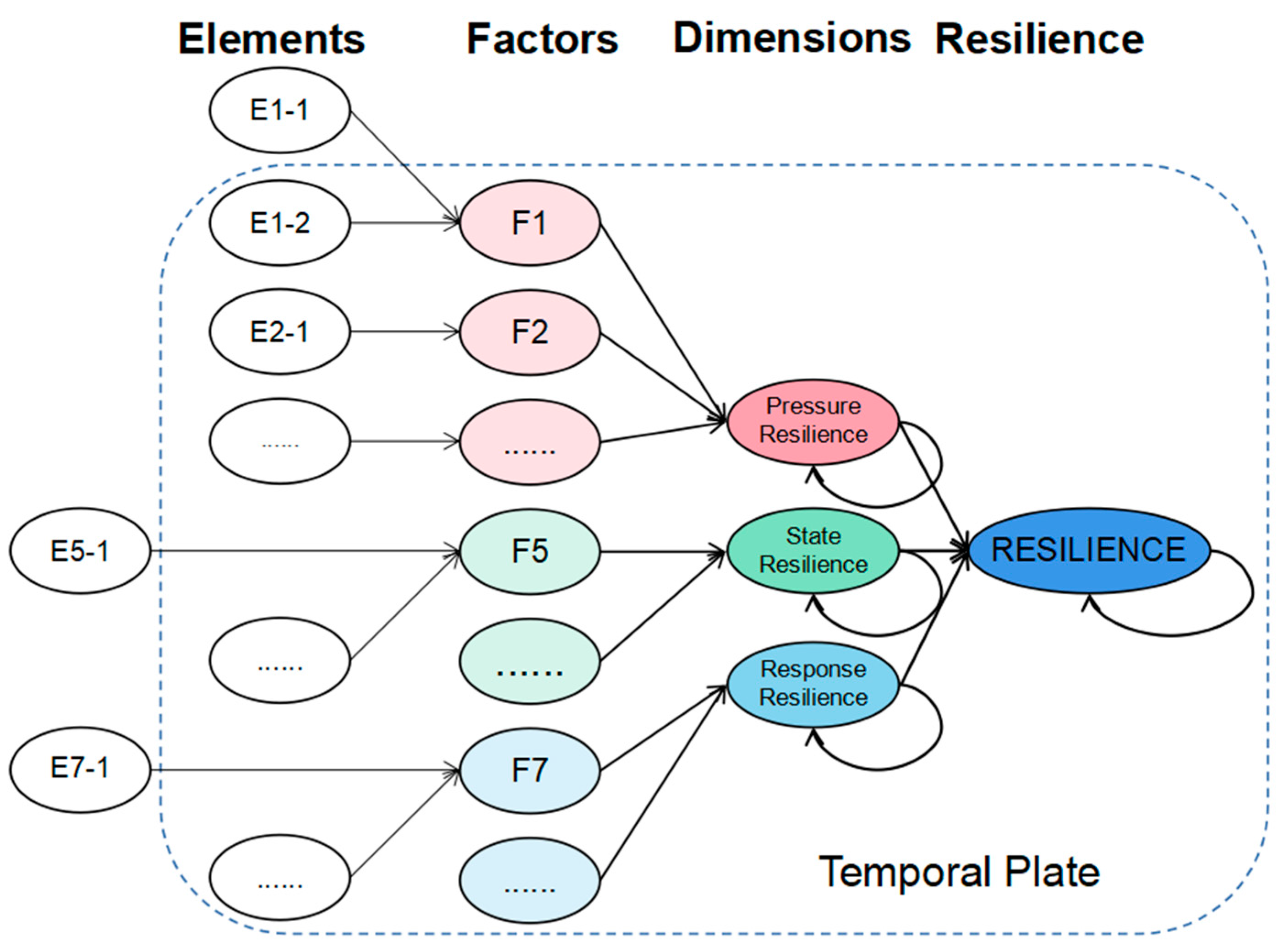
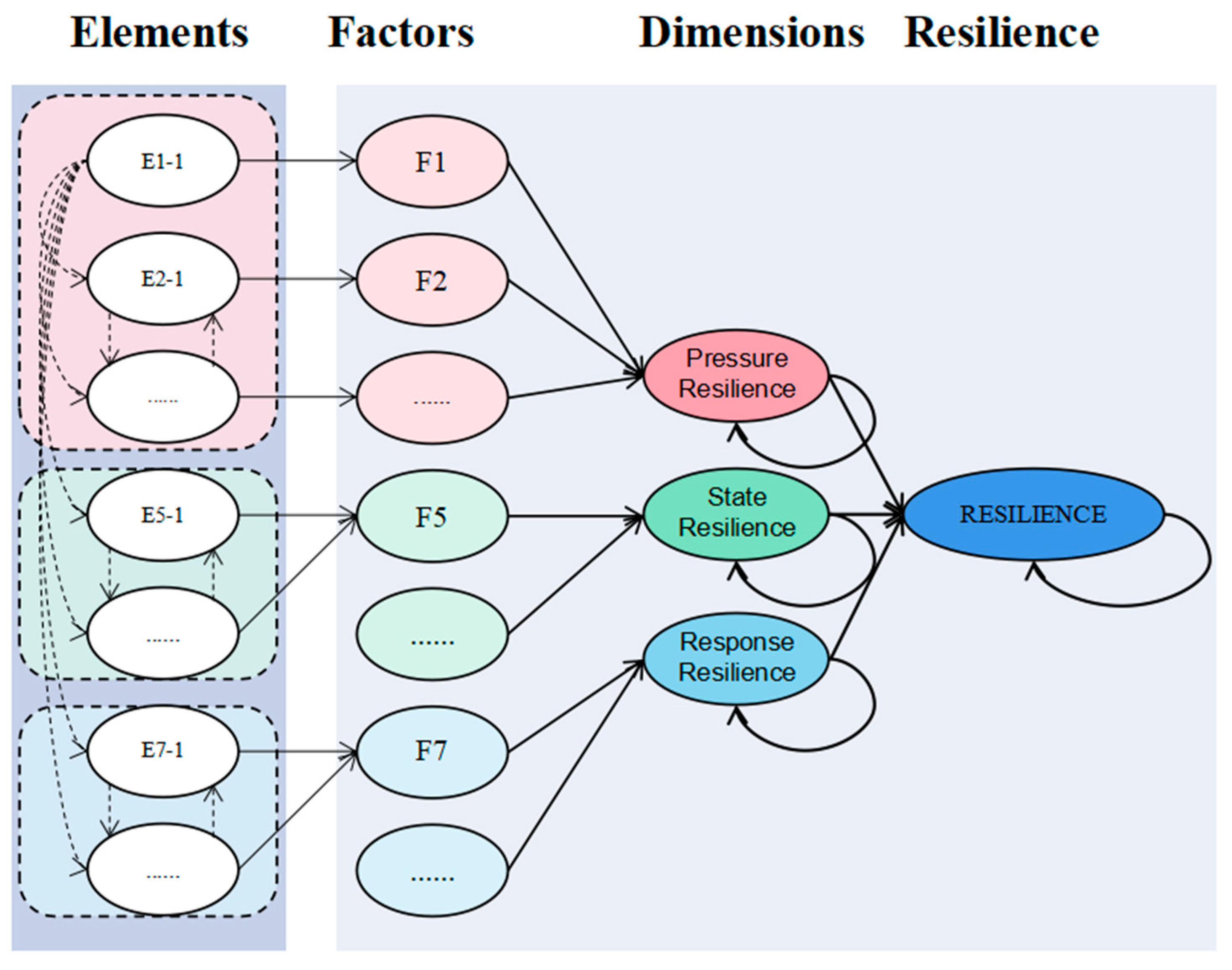
2. Road Operational Resilience

2.1. Definition of Road Operational Resilience

Road resilience refers to the ability of a road system to provide functional services when facing emergency events and disturbances sustainably. The pressure generated by emergency events and disturbances is the reason for the decline in the functional service capacity of the road system. The functional state presented by the road system in the face of disturbance pressure from different emergency events is determined by the performance of the comprehensive interference and resistance elements of the road system. The external behavior of restoring the functional service capacity of the road system is a response to the impact on the road. Therefore, the “pressure-state-response” framework could be used to abstract the evolutionary process of road resilience [37]. Therefore, this article proposes the concept of road operational resilience based on Pressure-State-Response (PSR) theory. In this paper, road resilience is defined as the ability of a road system to maintain functional status via its physical and topological properties, resist pressure, retain stability, and restore traffic capacity through emergency response to emergency events and disturbances. It focuses on the functional performance of engineering systems. It pays attention to the impact of external pressure and the recovery of functional status under intervention. Combining the resilience evolution mechanism, we divide it into three dimensions: pressure resilience, state resilience, and response resilience. Among them, pressure resilience characterizes the degree of disturbance stimulus when the road system operates. State resilience characterizes the stability of facilities in maintaining functions under disturbances. Response resilience measures the ability of road systems to recover from external responses.

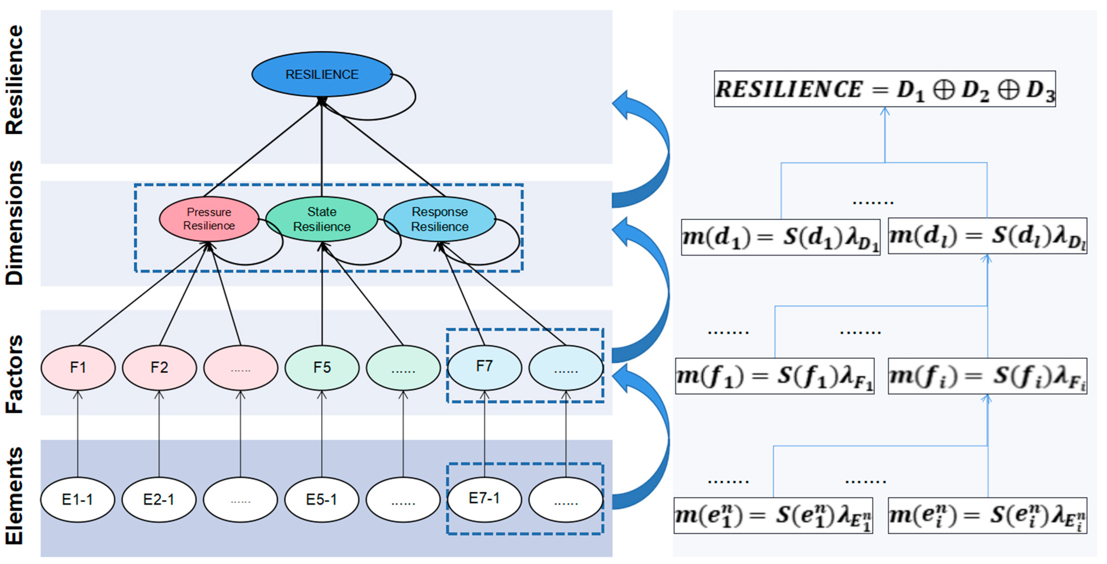
2.2. Analysis of Road Operational Resilience Elements

Road operational resilience is related to the environment, road, and facilities (such as the robustness of pavement performance, the robustness of lane access, and the robustness of facility functions). To more clearly depict road operational resilience, this paper proposes a hierarchical framework of road operational resilience elements based on PSR theory, as shown in Figure 1.

The pressure resilience dimension is characterized using exposure, uncertainty, diversity, and hazard factors related to pressure:

• The exposure to pressure characterizes the possibility of the road system being exposed to risk scenarios. The higher the exposure, the greater the possibility of disturbance. Specific elements include the exposure to meteorology (E1-1), the exposure to road type (E1-2), and the exposure to traffic flow (E1-3);
• The uncertainty of pressure characterizes the randomness of the time, type, and degree of emergency events on roads. The higher the uncertainty of pressure disturbance, the lower the pressure resilience performance, and the higher the difficulty for road systems to defend against disasters. Specific elements include the diversity of accident types (E2-1) and the diversity of vehicle types (E2-2);
• The diversity of pressures characterizes the possibility that road systems face various types of risks. Under the influence of other external factors, such as complex road environments and vehicle conditions, various disturbances may occur in a coupled and spread manner, increasing the risk of impact. Specific elements include uncertainty of scattered objects (E3-1) and uncertainty of fire (E3-2);
• The risk impact on road emergency occurrences is characterized by the pressure hazard, which includes losses of facilities, personnel, and vehicles. Specific elements include the hazards to the vehicle involved (E4-1), the hazards to casualties (E4-2), and the hazards to the facility (E4-3);

This paper measures the state resilience dimensions based on state robustness and state redundancy factors;

• The state of robustness is the ability of a road system’s inherent properties to resist disturbances, such as physical properties and network topology properties. Specific elements include the robustness of road width (E5-1), the robustness of road maintenance (E5-2), the robustness of pavement performance (E5-3), the robustness of lane access (E5-4), and the robustness of facility functions (E5-5);
• The state redundancy maintains functions through its replaceable components in response to damaged traffic functions. It is generally characterized by the storage capacity and substitutability of resources required by road systems, such as the redundancy of design traffic capacity (E6-1) and the redundancy of road network connectivity (E6-2).

This paper describes response resilience through response awareness, resourcefulness of response, rapidity of response, and responsive learnability:

• Response awareness characterizes the timeliness and accuracy of perception for emergency events and risk environments. It is a prerequisite for response occurrence and can be characterized by the rapidity of response arrival (E7-1);
• Rapidity of response refers to the ability of transportation system managers to take emergency disposal measures to restore system functions quickly. It usually manifests itself as effectiveness and speediness in emergency disposal. Specific elements include the implementability of response disposal (E8-1) and the rapidity of response disposal (E8-2);
• The resourcefulness of the response is measured by managers’ ability to organize transportation systems to establish priorities and mobilize various disaster prevention and mitigation resources. It is the basis for response disposal. Specific elements include the availability of rescue resources (E9-1), the availability of traction resources (E9-2), and the availability of firefighting resources (E9-3);
• The term responsive learnability refers to a transportation system’s ability to absorb historical experience and continuously learn so that functional status can be restored as soon as possible or even reach higher performance levels. It is characterized by emergency review capabilities (E10-1).

Road operational resilience is a dynamic, comprehensive result of elemental combinations in various dimensions. Its evolution also follows the stages of defense disturbance, resistance disturbance, and function repair [38]. As shown in

Table 1. Elements of road operational resilience for each resilience phase.

Dimen -sions	Factors	Elements of the Defense Disturbance Phase	Elements of the Resistance Disturbance Phase	Elements of the Functional Recovery Phase
Pressure resilience	Exposure to pressure	Exposure to meteorology(E1-1)
		Exposure to road types (E1-2)
		Exposure to traffic flows (E1-3)
	Diversity to pressure		Diversity of accident types (E2-1)
			Diversity of vehicle types (E2-2)
	Uncertainty of pressure		Uncertainty of scattered objects (E3-1)
			Uncertainty of fire (E3-2)
	Hazard of pressure		Hazardous to the facility (E4-1)
			Hazardous to the vehicle involved (E4-2)
			Hazardous to casualties (E4-3)
State resilience	State robustness		Robustness of road width (E5-1)
			Robustness of road maintenance (E5-2) Robustness of pavement performance (E5-3)
			Robustness of lane access (E5-4)
			Robustness of facility functions (E5-5)
	State redundancy		Redundancy of design traffic capacity (E6-1)
			Redundancy of road network connectivity (E6-2)
Response resilience	Response awareness		Rapidity of response arrival (E7-1)
	Rapidity of response			Implementability of response disposal (E8-1)
				Rapidity of response disposal (E8-2)
	Resourcefulness of response			Availability of rescue resources (E9-1)
				Availability of traction resources (E9-2)
				Availability of firefighting resources (E9-3)
	Responsive learnability			Emergency review capabilities (E10-1)

, in the defense disturbance stage, the road system faces risk scenarios under the influence of exposure to pressure elements. Under the action of elements in the diversity to pressure factor layer and the uncertainty of the pressure factor layer, the system’s performance is in a fluctuating stage. In the resistance disturbance stage, the system is affected by elements under the hazard of the pressure factor layer (such as those hazardous to casualties), and relying on its resources cannot defend against disturbance, and its performance rapidly declines. The speed of performance decline is related to elements under the state robustness and state redundancy factor layers (such as the redundancy of design traffic capacity and the redundancy of road network connectivity). The elements under the system’s response awareness factor layer also take effect at this stage. In the functional repair stage, elements under the resourcefulness of the response factor layer and the rapidity of the response factor layer (such as the availability of rescue resources and the rapidity of response disposal) take effect after perceiving on-site information and relying on elements under the responsive learnability factor layer (such as the emergency review capabilities) to improve decision quality. System performance begins to recover at this stage until it reaches road traffic performance requirements.

The interaction of elements under the dimensions of pressure resilience, state resilience, and response resilience is the direct cause of the change in road operational resilience. The blue arrow lines in Figure 2 show the interaction mechanism between elements. When a disturbance occurs, the elements under pressure resilience will stimulate the elements under state resilience in the road system. The system will mobilize the elements under state resilience to mitigate the impact of the elements under pressure resilience. A disturbance occurs if the road system fails to recover its functional status quickly. The operator of the road system will receive an assistance signal, make emergency decisions, mobilize resources, and take measures. Currently, the elements under response resilience act on the elements under state resilience to enhance the functional state of the road system. In addition, during the disturbance period, the emergency response subject of the road system receives disturbance information from elements under pressure resilience and takes preventive measures. At this time, the elements under response resilience will work on the elements under pressure resilience, minimizing the impact of disturbance pressure on the road system.

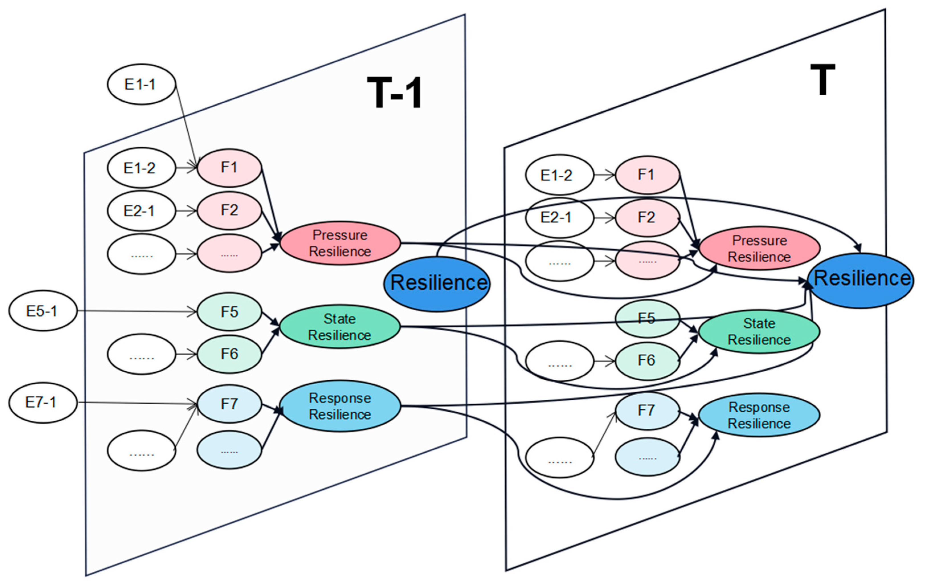
3. Road Operational Resilience Evolution Based on DBN

Road operational resilience is a complex concept that involves multiple factors, such as people, vehicles, and the environment. It dynamically changes with the development of emergency events, making it challenging to evaluate its resilience using conventional deterministic methods [39]. In this study, we consider the multidimensional impacts of pressure disturbances, state resistance, and response recovery faced by roads and establish a dynamic measurement method for resilience using Dynamic Bayesian Networks (DBN). DBN is a classical probabilistic graphical method that can address uncertainties in resilience measurement and balance multiple influencing factors to characterize resilience dynamically [40,41].

To construct the DBN, we first identify the relevant variables in the hierarchical framework of road operational resilience elements in Section 2.2 and use them as DBN nodes. Based on the hierarchical framework of resilience elements, we construct the basic structure of the DBN and determine the dependency relationships between resilience elements through structural learning using historical data from emergency events. Then, we determine the resilience state of network nodes using the Best Worst Method (BWM) and Dempster–Shafer (DS) evidence theory. We extend the resilience status dataset using historical data from emergency events and determine the strength of the dependency relationship between resilience elements through parameter learning. This DBN can be used to measure the evolution of road operational resilience.

To quantitatively calculate road operational resilience, we assign each node in the DBN a resilience state attribute divided into “good resilience” and “poor resilience” states. We measure the “good” and “poor” resilience states using the classical Bayesian network classification method [22,23], which significantly reduces the computational complexity of the model. We use the probability of maintaining “good resilience” or recovering from a “poor resilience” state to a “good resilience” state under emergency event scenarios as a measure of resilience. The probability values of resilience status can be used to compare resilience in different scenarios. We determine the resilience state of the resilience element node through the historical dataset of emergency events, with experts using domain knowledge to classify the data into “good resilience” and “poor resilience” states. We determine the probability value by calculating the frequency of “good resilience” states from historical data on emergency events. We identify the resilience factor node, resilience dimension node, and road operational resilience node based on the node state discrimination method proposed in Section 3.3.

3.1. Description of Road Emergency Event Data

The DBN’s nodes and attributes, network structure, and parameters all rely on historical data from road emergency events. Therefore, this study collected detailed historical data on road emergency events from Shanghai urban road operating enterprises. The original data was recorded and stored in tables and text form, as shown in

Table 2. Extraction of road emergency event data based on PSR.

Dimensions	Elements	Data of Elements
Pressure resilience	Exposure to meteorology	Weather conditions
	Exposure to road type	Road type of accident occurrence
	Exposure to traffic flow	Traffic flow
	Diversity of accident types	Accident type
	Diversity of vehicle types	Vehicle types
	Uncertainty of scattered objects	Scattered objects situation
	Uncertainty of fire	Fire situation
	Hazardous to facility losses	Facility losses
	Hazardous to the vehicle involved	Number of vehicles involved
	Hazardous to casualties	Casualty numbers
State resilience	Robustness of road width	Road width
	Robustness of road maintenance	Road maintenance situation
	Robustness of pavement performance	Pavement performance
	Robustness of lane access	Accessible lanes
	Robustness of facility functions	Facility functions
	Redundancy of road network connectivity	Road network connectivity
	Redundancy of design traffic capacity	Design traffic capacity
Response resilience	Response awareness	Accident discovery time
	Implementability of response disposal	Response arrival time
	Rapidity of response disposal	Disposal time
	Availability of rescue resources	Rescue resources
	Availability of traction resources	Traction resources
	Availability of firefighting resources	Firefighting resources
	Emergency review capabilities	Responsive learnability and review capacity

, and typical event records such as “At 00:50, with clear weather and traffic density of 200 pcu/km/ln, a one-compartment tanker truck collided with the guardrail on S20 inner ring to G50 ramp, causing damage to the guardrail and spillage of objects, occupying one lane without ignition and hindering the rear traffic. At 01:10, the towing vehicle arrived. At 01:15, one person was injured and sent for medical treatment. The ramp was temporarily closed, and the traffic behind was slow, with implementation difficulties. At 02:35, the accident was cleared, and the traffic resumed normal flow. There was no maintenance operation on the accident section”. Following the resilience element classification method in Section 2.2, relevant data were extracted from the pressure, state, and disturbance dimensions.

To better present the critical information in the data, this paper extracts event information from three dimensions: pressure, state, and disturbance, based on the resilience element division method described in Section 2.2:

• The pressure dimension data includes accident occurrence time, weather conditions, traffic flow during the incident, accident location, accident type, vehicle types, scattered objects situation, fire situation, facility losses, number of involved vehicles, and casualty numbers;
• The state dimension data includes road width, road maintenance situation, pavement performance, total lanes, occupied lanes, facility functions, road network connectivity, and design traffic capacity;
• The response dimension data encompasses accident discovery time, response arrival time, disposal time, response-related resources such as rescue, traction, firefighting resources, and accident logging time.

The historical data of emergency events includes continuous data related to time, such as handling time, and discrete data, such as casualty numbers and accident types. For discrete data, this study defines them as discrete variables by referencing the Chinese national standards“Codes for traffic accident information” (GA/T16.1-16.18-2010) [42], “Codes for Road Traffic Accident Scene” (GA 17.1–17.11-2003) [43], and expert knowledge. For instance, the number of injuries of two or fewer is converted to 0, while the number of injuries greater than two or the occurrence of severe injuries and deaths is labeled as 1. For continuous data, information about an event is recorded in units of 15 min, and a period of five time intervals (75 min) is considered one cycle based on the distribution of real-world data. With the guidance of expert experience, data values are assigned as good resilience status (0) and poor resilience status (1). For example, if the original data describes the handling of an incident as “At 00:50, with clear weather and traffic density of 200 pcu/km/ln, a one-compartment tanker truck collided with the guardrail on S20 inner ring to G50 ramp, causing damage to the guardrail and spillage of objects, occupying one lane without ignition, and hindering the rear traffic. At 01:10, the towing vehicle arrived. At 01:15, one person was injured and sent for medical treatment. The ramp was temporarily closed, and the traffic behind was slow, with implementation difficulties. At 02:35, the accident was cleared, and the traffic resumed normal flow. There was no maintenance operation on the accident section”, the emergency response time is the difference between the time the towing vehicle arrived and the time the incident was discovered, which falls under the time interval T1 (15 min)–T2 (30 min). The response perception in this period is beneficial for the resilience of road operations. It is assigned a value of 0, while the response perception in the 0–T1 time interval was not in place and is assigned a value of 1. Similarly, other data related to time are processed accordingly. After processing the data, as shown in

Table 3. The data on emergency events after processing.

Data of Elements	Emergency Event 1	Emergency Event 2	Emergency Event 3	Emergency Event 4	...
Weather conditions	0	0	1	1	...
Road type of accident occurrence	0	1	0	1	...
Traffic flow	1	1	1	1	...
Accident type	1	1	1	1	...
Vehicle types	0	0	0	0	...
Scattered objects situation	0	0	0	0	...
Fire situation	0	0	0	0	...
Facility losses	0	0	0	0	...
Number of vehicles involved	1	0	1	1	...
Casualty numbers	0	0	0	0	...
Road width	0	1	0	0	...
Road maintenance situation	0	0	0	0	...
Pavement performance	0	0	1	0	...
Accessible lanes	0	1	0	0	...
Facility functions	0	1	0	0	...
Road network connectivity	0	0	1	1	...
Design traffic capacity	0	1	0	0	...
Accident discovery time	0	0	0	0	...
Response arrival time	0	1	0	0	...
Disposal time	0	1	0	0	...
Rescue resources	0	0	0	0	...
Traction resources	0	1	0	0	...
Firefighting resources	0	0	0	0	...
Responsive learnability and review capacity	0	0	0	0	...

, it is used as the input for the DBN network nodes.

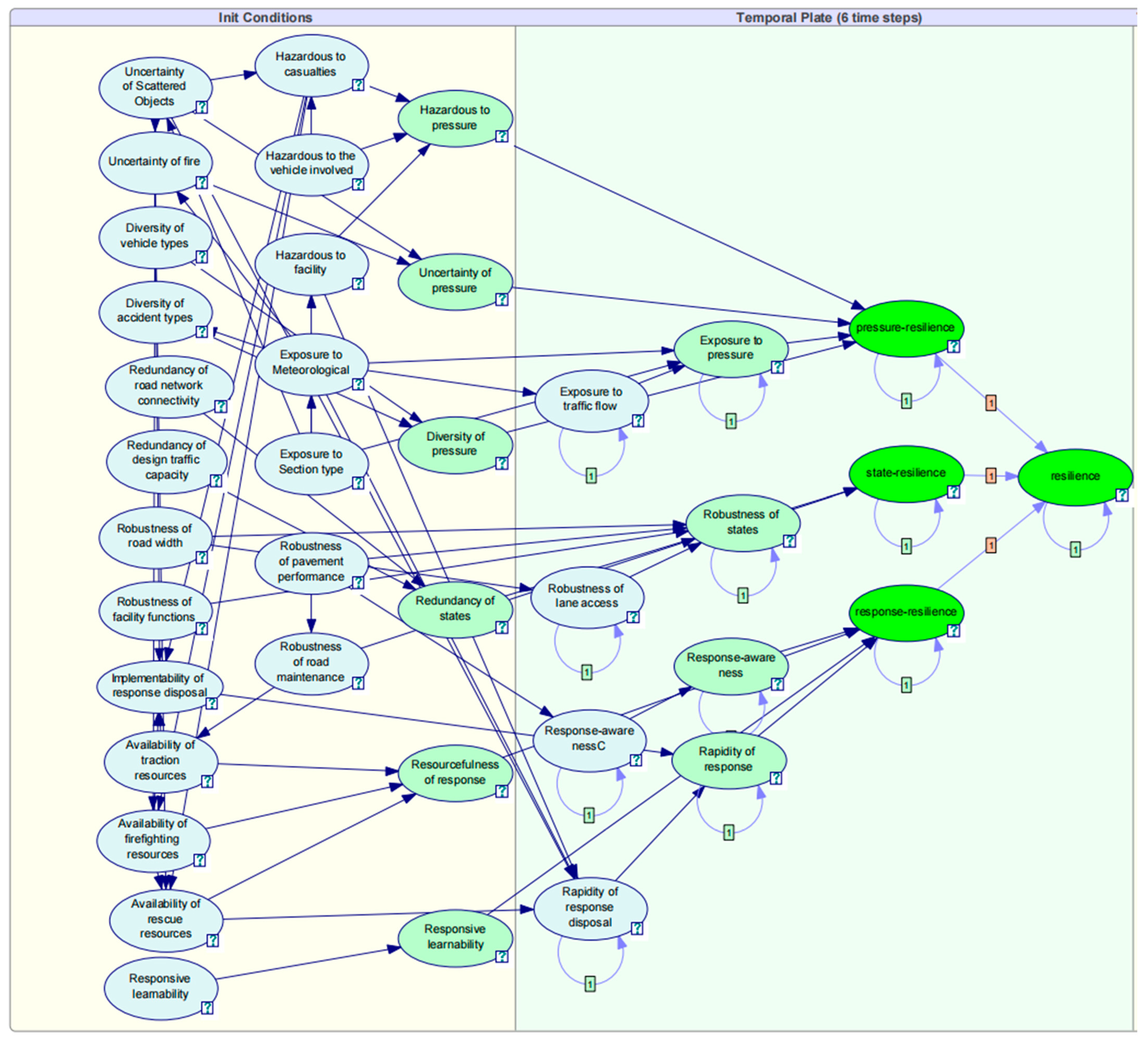
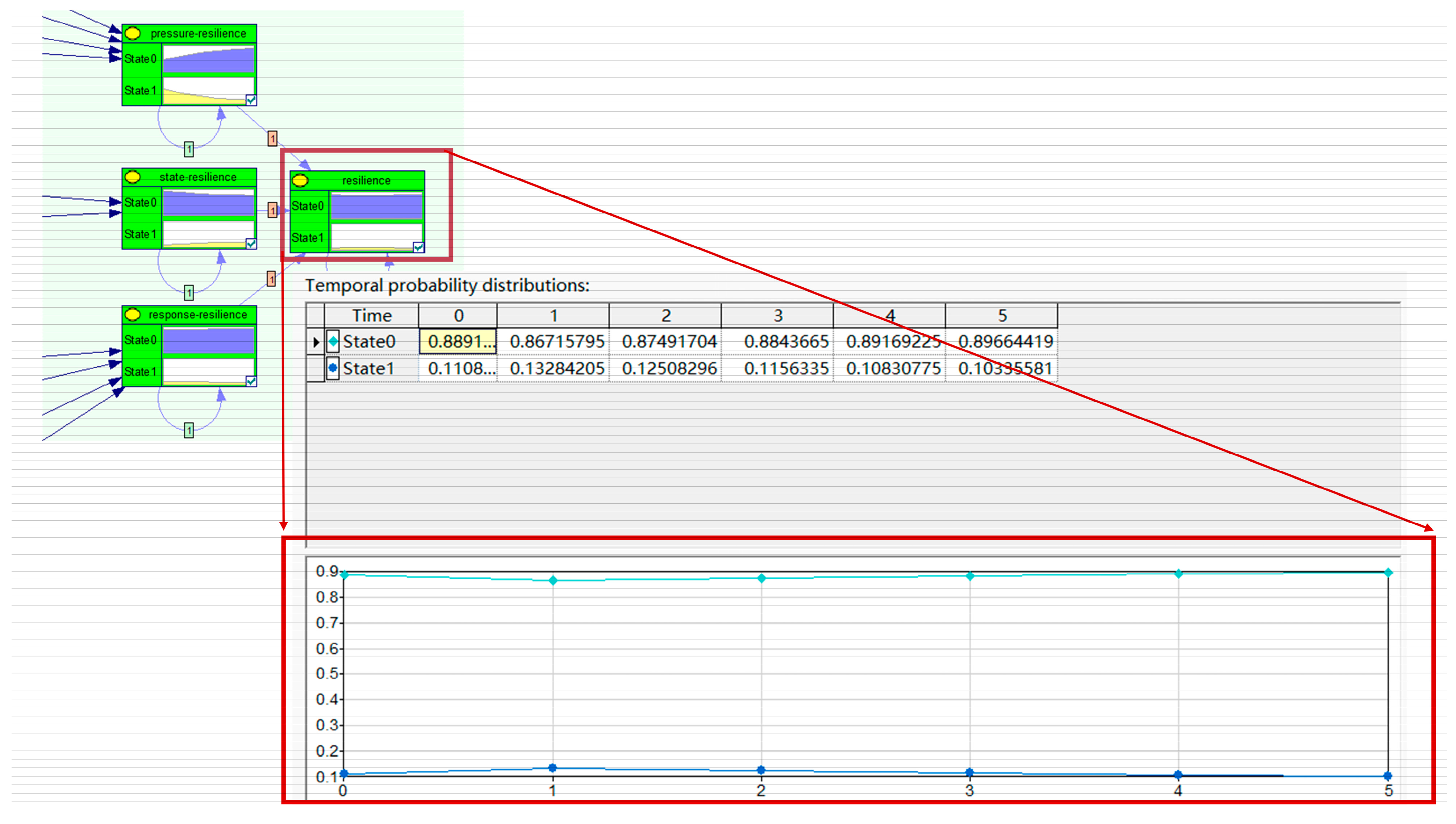
3.2. Construction of the DBN Structure for Resilience Evolution

First, according to the hierarchical framework of road operational resilience elements, an initial hierarchical Bayesian network structure is established, as shown in Figure 3. The nodes in the input layer correspond to the element hierarchy of the framework, specifically including nodes for specific elements of people, vehicles, roads, and environment (such as E1-1, E1-2, and E1-3). This hierarchical node type is an element type. The nodes in the middle layer correspond to the framework’s factor and dimension levels, so this layer’s node type is divided into factor and dimension types. Factor-type nodes include F1, F2, and F3 nodes. Dimension-type nodes include the pressure resilience nodes, the state resilience nodes, and the response resilience nodes. The nodes in the output layer correspond to the resilience level of the framework, and the RESILIENCE node represents the final road’s operational resilience. Then, the static relationship between each layer node is established according to the element attribution relationship of the element hierarchical framework. The RESILIENCE node connects to the middle layer’s pressure resilience node, state resilience node, and response resilience node. The pressure resilience node connects to the exposure to pressure node (F1), the pressure diversity node (F2), the uncertainty of pressure node (F3), and the pressure hazard (F4) node in factor-type nodes. The pressure hazard node connects to the hazardous to the vehicle involved (E4-1) node related to the input layer, the hazardous to casualties node (E4-2), and the hazardous to facilities node (E4-3). Similarly, the state resilience and response resilience nodes are constructed with corresponding middle layer factor-type nodes and input layer element-type nodes’ associations.

To portray the dynamic characteristics of resilience under the evolution of road operation scenarios, in this paper we first analyze whether network nodes have time-varying features (i.e., whether the values of variables corresponding to nodes change significantly over time). Based on domain knowledge and data obtained from scenarios, network nodes are divided into static nodes and dynamic nodes. For example, road width robustness (E5-1) is a static node that does not change with time. In contrast, lane traffic robustness (E5-4) changes with emergency events and on-site disposal and is a dynamic node. RESILIENCE nodes in the output layer, dimension nodes in the middle layer, and some factor nodes are all affected by input layer elements with time-varying features that are associated with them. Therefore, these nodes are listed as dynamic nodes.

Secondly, the resilience evolution mechanism is characterized by constructing associations between nodes at different time intervals. This paper assumes that the influence of nodes between different time intervals depends on the state of the previous time interval and that there is no influence across multiple time steps (reducing the complexity of node-time correlations and increasing computational feasibility) [20,22].

This paper divides the node relationships between different time slices into two categories: one is that nodes in T-time slices are influenced by their own nodes in T-1 time slices, such as RESILIENCE node status evolution based on the resilience status of this node in the previous time slice, for which connections between adjacent nodes of the same type are constructed. The other is that other nodes influence nodes in the T-time slice in the T-1 time slice. For example, the RESILIENCE node under the T-time slice also depends on the influence of the resilience state of the pressure resilience, the response resilience, and the state resilience nodes in the previous time slice. For this type of relationship, connections between this node and other nodes influenced by T-1 time slices are constructed. Figure 4 shows the resilience DBN structure considering node relationships between different time steps, and Figure 5 shows the expanded DBN structure.

In the road operation scenario, the relationships between various element nodes are too complicated to judge directly. The correlation between elements can be discovered based on historical data on emergency events. Then, the relationship between nodes at different levels of the element hierarchy can be improved to align the network structure with the evolution law of road resilience. This paper employs the Greedy Thick Thinning algorithm to learn the interactions between elements in the road unexpected event dataset [44], as shown in the dashed arrows in Figure 6, and improve the node relationship. The algorithm first initializes the correlation between all variables as none and then repeatedly performs the dense and sparse processes to find the optimal model structure. In each stage, the algorithm evaluates the model using the Bayesian information criterion (BIC) and selects the best model structure based on the score. Consequently, an accurate network structure is constructed to reflect the evolution of road resilience.

According to the phase characteristics analysis of resilience elements in Section 2.2, some characterization elements have time attributes and different action times, which are included in different time slices of the network. As shown in Figure 7, at the T0 moment, only static resilience elements are involved, such as the exposure to road type that characterizes the exposure to pressure, pavement performance that characterizes the state robustness, and initial resource reserves that characterize the resourcefulness of responses. At the T1 moment, elements that disrupt the function of the road system (e.g., fire uncertainty, object throwing uncertainty) are introduced, along with elements of state resilience that resist stress and maintain function (e.g., lane access robustness.) At the T2 moment, elements of the response resilience that restore function (e.g., response disposal timeliness) and elements of the response resilience that can sustainably enhance the function of the road system (e.g., responsive learnability) are introduced.

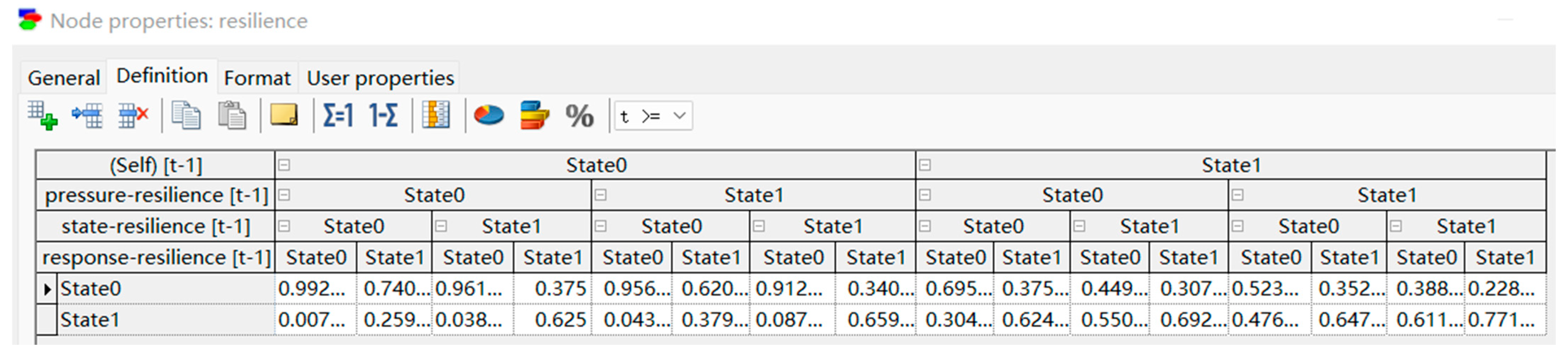
3.3. DBN Parameter Learning Based on Node Resilience Status

In addition to defining the network structure, it is essential to learn the parameters of a Dynamic Bayesian Network (DBN) to implement road operational resilience evolution based on dynamic Bayesian methods. DBN parameter learning involves determining the unconditional and conditional probabilities [45]. If a node in the network is not influenced by its parent nodes, it has an unconditional probability; on the other hand, if its parent nodes influence it, it has a conditional probability. The resilience status of input layer nodes can be gauged based on actual data and domain expertise, and their unconditional probability can be calculated based on the frequency of their resilience status. However, the resilience status of middle and output layer nodes cannot be directly obtained from recorded real-world data, making it crucial to initially determine the resilience status of these nodes before using data containing their resilience status to calculate their conditional probability.

Given the multiple factors that impact road operational resilience, two issues need to be addressed when determining the resilience status of each node. The first issue is determining the weightage of each influencing factor on the node’s resilience status. The second issue is how to incorporate numerous factors’ effects into determining the node’s resilience status. This paper proposes a method that utilizes the Best Worst Method (BWM) algorithm to convert domain knowledge into node weights and employs the Dempster–Shafer (DS) evidence theory to assess the resilience status of Bayesian network nodes by combining historical data on emergency events. Additionally, we have realized the BN parameter learning technique based on data.

When determining the weightage of each influencing factor concerning the resilience status of a node, we employ the BWM method. Compared to other multi-criteria decision-making methods, the BWM requires fewer pairwise comparisons between influencing factors, reducing the time required for analysis and producing more dependable results [46,47]. Thus, it is more appropriate for assessing the weights of various factors that affect road operational resilience. The influence weights of sub-nodes concerning parent nodes (i.e., the impact of parent nodes on sub-nodes) differ in determining the resilience status of middle and output layer nodes. Here, we use domain expertise to score the importance of parent nodes concerning sub-nodes and calculate the node weights using the BWM. The specific methodological process is outlined as follows:

• Expert ${\mathrm{P}}_{\mathrm{k}}$ selects the most important node ${\mathrm{C}}_{\mathrm{M}}^{\mathrm{k}}$ and the least important node ${\mathrm{C}}_{\mathrm{L}}^{\mathrm{k}}$ from a group of nodes $\mathrm{C}={\{\mathrm{C}}_1,{\mathrm{C}}_2,\cdots ,{\mathrm{C}}_{\mathrm{n}}\}$;
• The most important node ${\mathrm{C}}_{\mathrm{M}}^{\mathrm{k}}$ is compared with other nodes ${\mathrm{C}}_{\mathrm{j}}^{\mathrm{k}}\left(\mathrm{j}=\mathrm{1,2},\cdots ,\mathrm{n}\right)$ to determine their relative importance using a 1–9 scale, where higher values indicate greater importance, and to calculate the ratio ${\mathrm{V}}_{\mathrm{M}}^{\mathrm{k}}$ set as Equation (1)

  $$\begin{array}{c}{\mathrm{V}}_{\mathrm{M}}^{\mathrm{k}}=\left({\mathrm{v}}_{\mathrm{M}1}^{\mathrm{k}},{\mathrm{v}}_{\mathrm{M}2}^{\mathrm{k}},\cdots ,{\mathrm{v}}_{\mathrm{M}\mathrm{n}}^{\mathrm{k}}\right)\end{array}$$

  (1)

  where ${\mathrm{v}}_{\mathrm{M}\mathrm{j}}^{\mathrm{k}}$ represents the ratio of the importance of the most important node ${\mathrm{C}}_{\mathrm{M}}^{\mathrm{k}}$ chosen by ${\mathrm{P}}_{\mathrm{k}}$ to other nodes ${\mathrm{C}}_{\mathrm{j}}^{\mathrm{k}}(\mathrm{j}=\mathrm{1,2},...,\mathrm{n})$;
• The importance of other nodes ${\mathrm{C}}_{\mathrm{j}}^{\mathrm{k}}\left(\mathrm{j}=\mathrm{1,2},\cdots ,\mathrm{n}\right)$ is compared with the least important node ${\mathrm{C}}_{\mathrm{L}}^{\mathrm{k}}$ using the same scale. The ratio set ${\mathrm{V}}_{\mathrm{L}}^{\mathrm{k}}$ is calculated by Equation (2).

  $$\begin{array}{c}{\mathrm{V}}_{\mathrm{L}}^{\mathrm{k}}=\left({\mathrm{v}}_{1\mathrm{L}}^{\mathrm{k}},{\mathrm{v}}_{2\mathrm{L}}^{\mathrm{k}},\cdots ,{\mathrm{v}}_{\mathrm{n}\mathrm{L}}^{\mathrm{k}}\right)\end{array}$$

  (2)

  where ${\mathrm{v}}_{\mathrm{j}\mathrm{L}}^{\mathrm{k}}$ represents the ratio of the importance of other nodes ${\mathrm{C}}_{\mathrm{j}}^{\mathrm{k}}\left(\mathrm{j}=\mathrm{1,2},\cdots ,\mathrm{n}\right)$ to the least important node ${\mathrm{C}}_{\mathrm{L}}^{\mathrm{k}}$ selected by ${\mathrm{P}}_{\mathrm{k}}$;
• To obtain the optimal weight ${\mathsf{\alpha }}_{\mathrm{j}}^{\mathrm{k}}$, $\left|\frac{{\mathsf{\alpha }}_{\mathrm{M}}^{\mathrm{k}}}{{\mathsf{\alpha }}_{\mathrm{j}}^{\mathrm{k}}}-{\mathrm{v}}_{{\mathrm{M}}_{\mathrm{j}}}^{\mathrm{k}}\right|$ and $\left|\frac{{\mathsf{\alpha }}_{\mathrm{j}}^{\mathrm{k}}}{{\mathsf{\alpha }}_{\mathrm{L}}^{\mathrm{k}}}-{\mathrm{v}}_{\mathrm{j}\mathrm{L}}^{\mathrm{k}}\right|$ values should be minimized, and constraints should be set as Equation (3).

  $$\begin{gathered} \min \xi \\ \mathrm{s}.\mathrm{t}.\left|\frac{{\mathsf{\alpha }}_{\mathrm{M}}^{\mathrm{k}}}{{\mathsf{\alpha }}_{\mathrm{j}}^{\mathrm{k}}}-{\mathrm{v}}_{\mathrm{M}\mathrm{j}}^{\mathrm{k}}\right|⩽\mathsf{\xi },\mathrm{j}=\mathrm{1,2},\dots ,\mathrm{n} \\ \left|\frac{{\mathsf{\alpha }}_{\mathrm{j}}^{\mathrm{k}}}{{\mathsf{\alpha }}_{\mathrm{L}}^{\mathrm{k}}}-{\mathrm{v}}_{\mathrm{j}\mathrm{L}}^{\mathrm{k}}\right|⩽\mathsf{\xi },\mathrm{j}=\mathrm{1,2},\dots ,\mathrm{n} \\ {\sum }_{\mathrm{j}=1}^{\mathrm{n}}{\mathsf{\alpha }}_{\mathrm{j}}^{\mathrm{k}}=1,\mathrm{j}=\mathrm{1,2},\dots ,\mathrm{n} \\ {\mathsf{\alpha }}_{\mathrm{j}}^{\mathrm{k}}⩾0,\mathrm{j}=\mathrm{1,2},\dots ,\mathrm{n} \end{gathered}$$

  (3)

  where ${\mathsf{\alpha }}_{\mathrm{j}}^{\mathrm{k}}$ represents the weight of the $\mathrm{j}$th node given by expert ${\mathrm{P}}_{\mathrm{k}}$;
• Convert ratios into node weights, and finally aggregate expert ${\mathrm{P}}_{\mathrm{k}}$ opinions to obtain weights as in Equation (4), where ${\mathsf{\lambda }}_{\mathrm{k}}$ is the weight of expert ${\mathrm{P}}_{\mathrm{k}}$.

  $$\begin{array}{c}{\mathsf{\alpha }}_{\mathrm{j}}={\sum }_{\mathrm{k}=1}^{\mathrm{l}}{\mathsf{\lambda }}_{\mathrm{k}}{\mathsf{\alpha }}_{\mathrm{j}}^{\mathrm{k}}\end{array}$$

  (4)

As an example, the weights of pressure resilience, state resilience, and response resilience nodes are parent nodes of road operational resilience. Experts determine their weights by considering which factor impacts the final road’s operational resilience the most. Some experts believe that pressure resilience is the leading cause of fluctuations in road operational resilience. Thus, it is of high importance. On the other hand, response resilience is critical for road operational resilience recovery, while the impact of state resilience on road maintenance functionality is relatively low among these three factors. Therefore, response resilience is chosen as the most important node, and state resilience is chosen as the least important node. The importance of response resilience is compared with that of pressure and state resilience, respectively, and the importance of pressure and response resilience is also compared with that of state resilience. Finally, the ratios between nodes are transformed into weights using Equations (3) and (4). The process of evaluating node weights is presented in

Table 4. Process for evaluating node weights using the BWM algorithm.

Method Step	Detailed Description of Each Step
Step 1	Criteria number = 3	Criterion 1	Criterion 2	Criterion 3
	Names of criteria	Pressure resilience	State resilience	Response resilience
	Select the best	Response resilience
	Select the worst	State resilience
Step 2	Names of criteria	Pressure resilience	State resilience	Response resilience
	Best to others	2	3	1
Step 3	Others to the worst	2	1	4
Step 4 and Step 5	Calculate node weights	0.27	0.16	0.57

. The weight calculation process for other nodes follows a similar approach.

After obtaining the node weights, the challenge is integrating multiple factors’ impacts on a node’s resilience state. Determining the resilience state requires integrating diverse information on influencing factors, which is inherently subjective and thus generates uncertainty [48]. However, the Dempster–Shafer (DS) evidence theory can overcome this issue by combining evidence [29]. DS evidence theory is precious when assessing road operational resilience, which involves multiple elements and hierarchical data [49]. This paper adopts a layered approach based on the DS evidence theory to tackle this challenge. First, the resilience-related variables of secondary-element nodes are combined at the factor node level. Then, the resilience state of factor nodes is integrated into the resilience state of dimension nodes. Finally, the resilience state of dimension nodes is merged into the resilience state of road operational resilience nodes. This comprehensive evaluation enables the determination of the resilience states of all nodes. The process includes the following steps:

• Determine the identification framework $\mathsf{\Theta }$ and construct a non-empty set of resilience element states. In this paper, the states of road operational resilience elements are conducive to resilience ($\mathrm{H}$) and detrimental to resilience evaluation ($\mathrm{L}$). All sets of identification framework $\mathsf{\Theta }=\{\mathrm{L},\mathrm{H}\}$ are called the power set $2^{\mathsf{\Theta }}$, and their subsets are called focal elements.

  $$\begin{array}{c}{2}^{\mathsf{\Theta }}=\left\{\mathsf{\phi },\mathrm{L},\mathrm{H},\left\{\mathrm{L},\mathrm{H}\right\}\right\};\end{array}$$

  (5)
• Assign confidence between 0 and 1 to focal elements within the identification framework, determining the Basic Probability Assignment or mass function $\mathrm{m}\left(\mathrm{A}\right)$ as Equation (6).

  $$\begin{array}{c}{\displaystyle \sum _{\mathrm{A}\subseteq \Theta }}\mathrm{m}\left(\mathrm{A}\right)=1\\ \forall \mathrm{A}\subseteq \mathsf{\Theta },0\le \mathrm{m}\left(\mathrm{A}\right)\le 1\end{array}$$

  (6)
• The Dempster–Shafer combination rule is used to combine two independent mass functions. This method gives us the fusion result ${\mathrm{m}}_{\mathrm{1,2}}\left(\mathrm{A}\right)$ of the parent node’s resilience status and the upper-level node’s resilience status. The calculations are as in Equations (7)–(9).

  $$\begin{array}{c}{\mathrm{m}}_{\mathrm{1,2}}\left(\mathrm{A}\right)={\mathrm{m}}_1\left(\mathrm{A}\right)\oplus {\mathrm{m}}_2\left(\mathrm{A}\right)\end{array}$$

  (7)

  $$\begin{array}{c}{\mathrm{m}}_{12}\left(\mathrm{A}\right)=\left\{\begin{array}{l}\frac{{\sum }_{\mathrm{X}\cap \mathrm{Y}=\mathrm{A},\forall \mathrm{X},\mathrm{Y}\subseteq \mathsf{\Theta }}{\mathrm{m}}_1\left(\mathrm{X}\right){\mathrm{m}}_2\left(\mathrm{Y}\right)}{1-\mathrm{K}}\\ 0,\mathrm{A}=\mathsf{\Phi }\end{array},\mathrm{A}\ne \mathsf{\Phi }\right.\end{array}$$

  (8)

  $$\begin{array}{c}\mathrm{K}={\sum }_{\mathrm{X}\cap \mathrm{Y}=\mathsf{\Phi }}{\mathrm{m}}_1\left(\mathrm{X}\right){\mathrm{m}}_2\left(\mathrm{Y}\right)<1\end{array}$$

  (9)

where $\mathrm{K}$ represents conflicts between subset $\mathrm{X}$ and subset $\mathrm{Y}$.

For the fusion of resilience states across multiple nodes, combining the states of multiple nodes is possible as the node combination sequence does not affect the result in the DS evidence theory [50]. The process involves layering the resilience states of multiple nodes and fusing them in a hierarchical framework of resilience elements, as shown in Figure 8. The rule for fusing the resilience state of an element node into the resilience state of a factor node can be expressed as Equations (10) and (11), whereas the rule for fusing the resilience state of a factor node into the resilience state of a dimension node can be expressed as Equations (12) and (13). Finally, the rule for fusing the resilience state of a dimension node into the resilience state of the road operational resilience node can be expressed as Equations (14) and (15).

$$\begin{array}{c}\mathrm{m}\left({\mathrm{e}}_{\mathrm{i}}^{\mathrm{n}}\right)=\mathrm{S}\left({\mathrm{e}}_{\mathrm{i}}^{\mathrm{n}}\right){\mathsf{\lambda }}_{{\mathrm{E}}_{\mathrm{i}}^{\mathrm{n}}}\end{array}$$

(10)

$$\begin{array}{c}{\mathrm{F}}_{\mathrm{i}}={\mathrm{E}}_{\mathrm{i}}^1\oplus {\mathrm{E}}_{\mathrm{i}}^2\oplus \dots \oplus {\mathrm{E}}_{\mathrm{i}}^{\mathrm{n}}\end{array}$$

(11)

where $\mathrm{m}\left({\mathrm{e}}_{\mathrm{i}}^{\mathrm{n}}\right)$ represents the mass function of state for the n-th element node under the i-th factor. $\mathrm{S}\left({\mathrm{e}}_{\mathrm{i}}^{\mathrm{n}}\right)$ evaluates the resilience status of the corresponding element node, while ${\mathsf{\lambda }}_{{\mathrm{E}}_{\mathrm{i}}^{\mathrm{n}}}$ represents the weight of the corresponding element node. ${\mathrm{F}}_{\mathrm{i}}$ denotes the resilience status of the i-th factor node, and ${\mathrm{E}}_{\mathrm{i}}^{\mathrm{n}}$ represents the resilience status of the n-th element node that influences ${\mathrm{F}}_{\mathrm{i}}$. The combination of the resilience status of the n element nodes (${\mathrm{E}}_{\mathrm{i}}^1$ ${\mathrm{E}}_{\mathrm{i}}^2$, …, ${\mathrm{E}}_{\mathrm{i}}^{\mathrm{n}}$) is used to calculate the resilience status of the i-th factor node, ${\mathrm{F}}_{\mathrm{i}}$.

$$\begin{array}{c}\mathrm{m}\left({\mathrm{f}}_{\mathrm{i}}\right)=\mathrm{S}\left({\mathrm{f}}_{\mathrm{i}}\right){\mathsf{\lambda }}_{{\mathrm{F}}_{\mathrm{i}}}\end{array}$$

(12)

$$\begin{array}{c}{\mathrm{D}}_{\mathrm{l}}={\mathrm{F}}_1\oplus {\mathrm{F}}_2\oplus \dots \oplus {\mathrm{F}}_{\mathrm{i}}\end{array}$$

(13)

where $\mathrm{m}\left({\mathrm{f}}_{\mathrm{i}}\right)$ represents the mass function of the i-th factor node. $\mathrm{S}\left({\mathrm{f}}_{\mathrm{i}}\right)$ evaluates the resilience status of the corresponding factor node, while ${\mathsf{\lambda }}_{{\mathrm{F}}_{\mathrm{i}}}$ represents the weight of the corresponding factor node. The combination of the resilience status of the i factor nodes generates the resilience status of the l-th dimension node, ${\mathrm{D}}_{\mathrm{l}}$.

$$\begin{array}{c}\mathrm{m}\left({\mathrm{d}}_{\mathrm{l}}\right)=\mathrm{S}\left({\mathrm{d}}_{\mathrm{l}}\right){\mathsf{\lambda }}_{{\mathrm{D}}_{\mathrm{l}}}\end{array}$$

(14)

$$\begin{array}{c}\mathrm{RESILIENCE}={\mathrm{D}}_1\oplus {\mathrm{D}}_2\oplus {\mathrm{D}}_3\end{array}$$

(15)

where $\mathrm{m}\left({\mathrm{d}}_{\mathrm{l}}\right)$ represents the mass function of state for the l-th dimension node.$\mathrm{S}\left({\mathrm{d}}_{\mathrm{l}}\right)$ evaluates the resilience status of the corresponding dimension node, while ${\mathsf{\lambda }}_{{\mathrm{D}}_{\mathrm{l}}}$ denotes the weight of the corresponding dimension node. By combining the resilience statuses of all three-dimensional nodes (${\mathrm{D}}_1$, ${\mathrm{D}}_2$, $\mathrm{a}\mathrm{n}\mathrm{d} {\mathrm{D}}_3$), we can obtain the resilience status of the RESILIENCE node.

Finally, the determination of the conditional probability of the DBN is completed by parameter learning with the EM algorithm [51] based on the historical data of emergency events and the judgment data of the node resilience state. In the EM algorithm, the E-step employs the Bayesian formula to calculate the posterior probability distribution of each variable for an emergency event. For a given node, its posterior distribution refers to the posterior probability of it taking different values under the condition of observing the data of all other nodes. In the M-step, we calculate the logarithmic likelihood function based on all known data and maximize this function to update the estimated values of the conditional probability table. The maximum likelihood estimation method can be used to achieve this process.

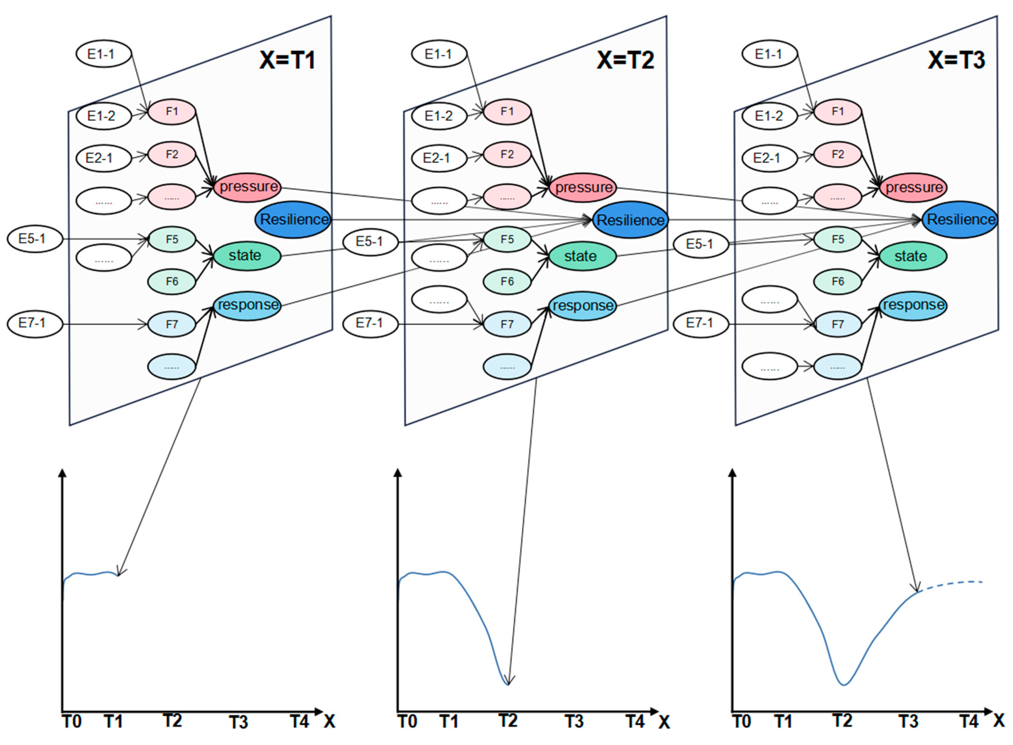
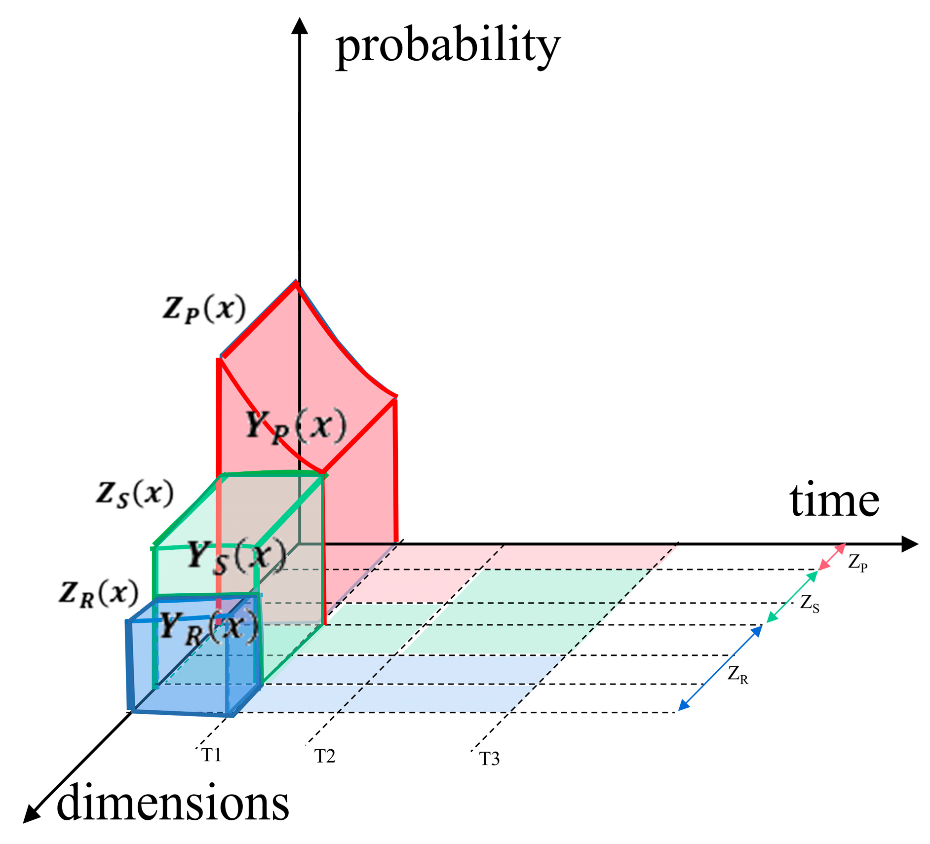
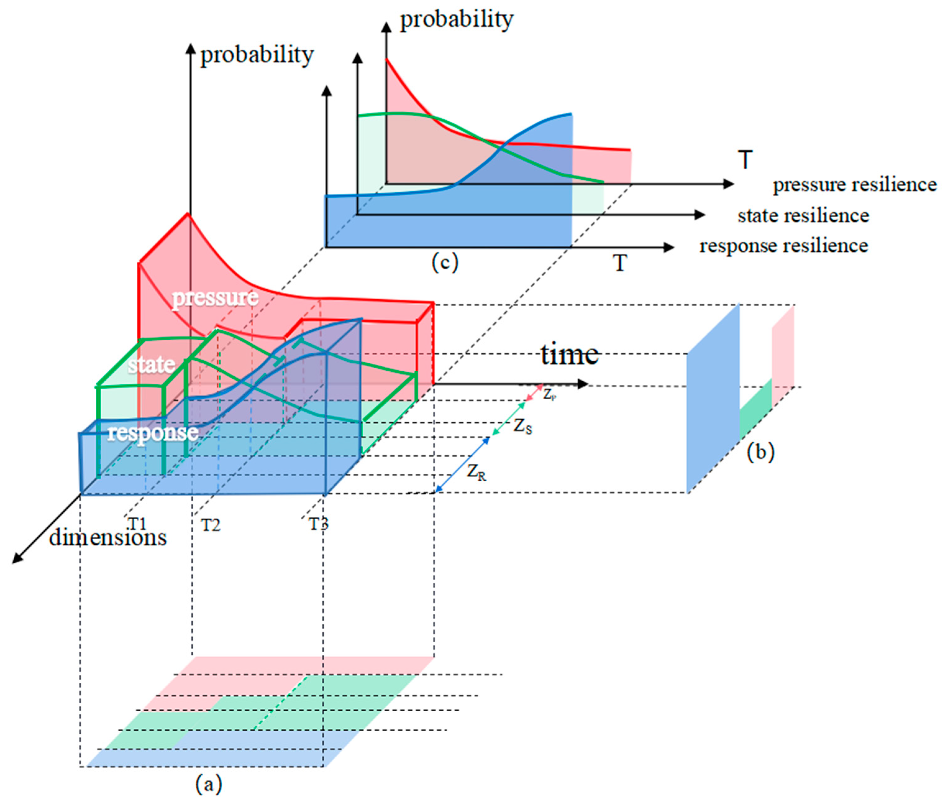
4. Multidimensional Integration and Visualization of Road Operational Resilience Evaluation

This chapter employs the methods introduced in Section 3 to quantify the pressure, state, response, and road operational resilience under emergency scenarios. The pressure resilience, ${\mathrm{Y}}_{\mathrm{P}}\left(\mathrm{t}\right),$ is quantified by the probability of changes in the pressure resilience state. Similarly, the state resilience ${\mathrm{Y}}_{\mathrm{S}}\left(\mathrm{t}\right)$ and response resilience ${\mathrm{Y}}_{\mathrm{R}}\left(\mathrm{t}\right)$ are measured by the probability of changes in their respective resilience states. These probabilities are obtained through DBN network learning and parameter learning based on resilience state judgment on the emergency event dataset, as described in Section 3. The pressure resilience, ${\mathrm{Y}}_{\mathrm{P}}\left(\mathrm{t}\right)$ at time $\mathrm{x}=\mathrm{t}$ is not only affected by the factors under the corresponding dimension at time $\mathrm{x}=\mathrm{t}-1$ but is also related to the pressure resilience ${\mathrm{Y}}_{\mathrm{P}}\left(\mathrm{t}-1\right)$ at time $\mathrm{x}=\mathrm{t}-1$. The factors $\left({\mathrm{H}}_1(\mathrm{t}-1),{\mathrm{H}}_2(\mathrm{t}-1),\dots ,{\mathrm{H}}_{\mathrm{n}}(\mathrm{t}-1)\right)$, and ${\mathrm{Y}}_{\mathrm{P}}\left(\mathrm{t}-1\right)$ are used as parent nodes of the pressure resilience ${\mathrm{Y}}_{\mathrm{P}}\left(\mathrm{t}\right)$, and the impact strength between nodes is measured by conditional probability. Therefore, the calculation of pressure resilience ${\mathrm{Y}}_{\mathrm{P}}\left(\mathrm{t}\right)$ is shown in Equation (16). Similarly, the calculation of state resilience ${\mathrm{Y}}_{\mathrm{S}}\left(\mathrm{t}\right)$ and response resilience ${\mathrm{Y}}_{\mathrm{R}}\left(\mathrm{t}\right)$ is shown in Equations (17) and (18).

$${\mathrm{Y}}_{\mathrm{P}}\left(\mathrm{t}\right)=\mathrm{P}\left({{\mathrm{H}}_1\left(\mathrm{t}\right),{\mathrm{H}}_2\left(\mathrm{t}\right),...,\mathrm{H}}_{\mathrm{i}}\left(\mathrm{t}\right)\right)={\prod }_{\mathrm{i}=1}^{\mathrm{n}} \mathrm{P}\left({\mathrm{H}}_{\mathrm{i}}\left(\mathrm{t}\right)\mid {\mathrm{P}\mathrm{a}(\mathrm{H}}_{\mathrm{i}}(\mathrm{t}-1)),{\mathrm{Y}}_{\mathrm{P}}(\mathrm{t}-1),\right)$$

(16)

$${\mathrm{Y}}_{\mathrm{S}}\left(\mathrm{t}\right)=\mathrm{P}\left({{\mathrm{S}}_1\left(\mathrm{t}\right),{\mathrm{S}}_2\left(\mathrm{t}\right),...,\mathrm{S}}_{\mathrm{i}}\left(\mathrm{t}\right)\right)={\prod }_{\mathrm{i}=1}^{\mathrm{n}} \mathrm{P}\left({\mathrm{S}}_{\mathrm{i}}\left(\mathrm{t}\right)\mid {\mathrm{P}\mathrm{a}(\mathrm{S}}_{\mathrm{i}}(\mathrm{t}-1)),{\mathrm{Y}}_{\mathrm{S}}(\mathrm{t}-1),\right)$$

(17)

$${\mathrm{Y}}_{\mathrm{R}}\left(\mathrm{t}\right)=\mathrm{P}\left({{\mathrm{R}}_1\left(\mathrm{t}\right),{\mathrm{R}}_2\left(\mathrm{t}\right),...,\mathrm{R}}_{\mathrm{i}}\left(\mathrm{t}\right)\right)={\prod }_{\mathrm{i}=1}^{\mathrm{n}} \mathrm{P}\left({\mathrm{R}}_{\mathrm{i}}\left(\mathrm{t}\right)\mid {\mathrm{P}\mathrm{a}(\mathrm{R}}_{\mathrm{i}}(\mathrm{t}-1)),{\mathrm{Y}}_{\mathrm{R}}(\mathrm{t}-1),\right)$$

(18)

${\mathrm{Y}}_{\mathrm{P}}\left(\mathrm{t}\right)$, ${\mathrm{Y}}_{\mathrm{S}}\left(\mathrm{t}\right)$, and ${\mathrm{Y}}_{\mathrm{R}}\left(\mathrm{t}\right)$ represent the probability that the status of the pressure resilience, the state resilience, and the response resilience at time $\mathrm{t}$. ${\mathrm{H}}_{\mathrm{n}},{\mathrm{S}}_{\mathrm{n}},$ and ${\mathrm{R}}_{\mathrm{n}}$ represent the $\mathrm{n}$th elements that affect pressure resilience, state resilience, and response resilience.

The road operational resilience, $\mathrm{R}\mathrm{e}\mathrm{s}\mathrm{i}\mathrm{l}\mathrm{i}\mathrm{e}\mathrm{n}\mathrm{c}\mathrm{e}\left(\mathrm{t}\right),$ at time t is affected by the pressure resilience ${\mathrm{Y}}_{\mathrm{P}}\left(\mathrm{t}-1\right)$, the state resilience ${\mathrm{Y}}_{\mathrm{S}}\left(\mathrm{t}-1\right)$, the response resilience ${\mathrm{Y}}_{\mathrm{R}}\left(\mathrm{t}-1\right)$ at time $\mathrm{t}-1$, and the road operational resilience, $\mathrm{R}\mathrm{e}\mathrm{s}\mathrm{i}\mathrm{l}\mathrm{i}\mathrm{e}\mathrm{n}\mathrm{c}\mathrm{e}\left(\mathrm{t}-1\right)$, at the previous time, calculated as Equation (19):

$$\mathrm{R}\mathrm{e}\mathrm{s}\mathrm{i}\mathrm{l}\mathrm{i}\mathrm{e}\mathrm{n}\mathrm{c}\mathrm{e}\left(\mathrm{t}\right)=\mathrm{P}\left({\mathrm{Y}}_{\mathrm{P}}(\mathrm{t}-1),{\mathrm{Y}}_{\mathrm{S}}(\mathrm{t}-1),{\mathrm{Y}}_{\mathrm{R}}(\mathrm{t}-1),\mathrm{R}\mathrm{e}\mathrm{s}\mathrm{i}\mathrm{l}\mathrm{i}\mathrm{e}\mathrm{n}\mathrm{c}\mathrm{e}(\mathrm{t}-1).\right)$$

(19)

In order to achieve quantitative visualization of multidimensional resilience with weight information at different stages in space, this paper proposes a method of multi-dimensional resilience evaluation, integration, and visualization. The two-dimensional x-y coordinate plane of the resilience curve model is expanded into an x-y-z spatial coordinate system. In this system, the x-axis (horizontal axis) represents time, and the y-axis (vertical axis) replaces the system performance value in the resilience curve model with the probability of dimension node resilience status being in good condition. By introducing a weight for each dimension of resilience, the degree of impact on road operational resilience can be quantified. The z-axis (depth axis) is incorporated to depict changes in the weight of each dimension of resilience over time. In the resilience curve model, the area of the function curve envelope of system performance concerning time represents the resilience for a certain period. As for the three-dimensional space constructed in this paper, by expanding the two-dimensional curves of the different dimensions of resilience with the corresponding weight in the z-axis direction, the spatial geometric bodies with each dimension of resilience are formed. The volume of spatial geometric bodies can reflect multidimensional resilience for a certain period, such as in Equations (20) and (21). It maps the state space of multidimensional resilience from 0-T1 to three-dimensional spatial geometric bodies, as shown in Figure 9.

$$\begin{gathered} \mathrm{V}\left(\mathrm{x},\mathrm{y},\mathrm{z}\right)={\int }_0^{{\mathrm{Z}}_{\mathrm{P}}\left(\mathrm{x}\right)}{\int }_0^{{\mathrm{T}}_1}{\mathrm{Y}}_{\mathrm{P}}\left(\mathrm{x}\right)\hspace{0.17em}\mathrm{dxdz}+{\int }_{{\mathrm{Z}}_{\mathrm{P}}\left(\mathrm{x}\right)}^{{\mathrm{Z}}_{\mathrm{P}}\left(\mathrm{x}\right)+{\mathrm{Z}}_{\mathrm{S}}\left(\mathrm{x}\right)}{\int }_0^{{\mathrm{T}}_1}{\mathrm{Y}}_{\mathrm{S}}\left(\mathrm{x}\right)\mathrm{dxdz} \\ +{\int }_{{\mathrm{Z}}_{\mathrm{P}}\left(\mathrm{x}\right)+{\mathrm{Z}}_{\mathrm{S}}\left(\mathrm{x}\right)}^1{\int }_0^{{\mathrm{T}}_1}{\mathrm{Y}}_{\mathrm{R}}\left(\mathrm{x}\right)\mathrm{d}\mathrm{x}\mathrm{d}\mathrm{z}, \end{gathered}$$

(20)

$${\mathrm{Z}}_{\mathrm{P}}\left(\mathrm{x}\right)+{\mathrm{Z}}_{\mathrm{S}}\left(\mathrm{x}\right)+{\mathrm{Z}}_{\mathrm{R}}\left(\mathrm{x}\right)=1,$$

(21)

where $\mathrm{x}$ represents a time value. The $\mathrm{z}$ represents the weight of different resilience dimensions, including pressure resilience ${\mathrm{Z}}_{\mathrm{P}}\left(\mathrm{x}\right)$, state resilience ${\mathrm{Z}}_{\mathrm{S}}\left(\mathrm{x}\right)$, and response resilience ${\mathrm{Z}}_{\mathrm{P}}\left(\mathrm{x}\right)$, on road operational resilience at a given time $\mathrm{x}$. $\mathrm{z}\in \left[0,{\mathrm{Z}}_{\mathrm{P}}\left(\mathrm{x}\right)\right]$, $\mathrm{z}$ falls within the range of influence for pressure resilience. $\mathrm{z}\in \left[{\mathrm{Z}}_{\mathrm{P}}\left(\mathrm{x}\right),{\mathrm{Z}}_{\mathrm{P}}\left(\mathrm{x}\right)+{\mathrm{Z}}_{\mathrm{S}}\left(\mathrm{x}\right)\right]$, $\mathrm{z}$ falls within the range of influence for state resilience. $\mathrm{z}\in \left[{\mathrm{Z}}_{\mathrm{P}}\left(\mathrm{x}\right)+{\mathrm{Z}}_{\mathrm{S}}\left(\mathrm{x}\right),1\right]\left(\mathrm{x}\right)$, $\mathrm{z}$ falls within the range of influence for response resilience. The $\mathrm{y}$ represents the probability of good status for each resilience dimension. $\mathrm{z}\in \left[0,{\mathrm{Z}}_{\mathrm{P}}\left(\mathrm{x}\right)\right]$, ${\mathrm{y}=\mathrm{Y}}_{\mathrm{P}}\left(\mathrm{x}\right)$, ${\mathrm{Y}}_{\mathrm{P}}\left(\mathrm{x}\right)$ represents the probability of good pressure resilience at time $\mathrm{x}$. $\mathrm{z}\in \left[{\mathrm{Z}}_{\mathrm{P}}\left(\mathrm{x}\right),{\mathrm{Z}}_{\mathrm{P}}\left(\mathrm{x}\right)+{\mathrm{Z}}_{\mathrm{S}}\left(\mathrm{x}\right)\right],{\mathrm{y}=\mathrm{Y}}_{\mathrm{S}}\left(\mathrm{x}\right),{\mathrm{Y}}_{\mathrm{S}}\left(\mathrm{x}\right)$ represents the probability of good state resilience at time $\mathrm{x}$. $\mathrm{z}\in \left[{\mathrm{Z}}_{\mathrm{P}}\left(\mathrm{x}\right)+\mathrm{Z}\mathrm{s}\left(\mathrm{x}\right),1\right]$, ${\mathrm{y}=\mathrm{Y}}_{\mathrm{R}}\left(\mathrm{x}\right)$, ${\mathrm{Y}}_{\mathrm{R}}\left(\mathrm{x}\right)$ represents the probability of good response resilience at time $\mathrm{x}$.

When evaluating road operational resilience, it is necessary to consider the weight of different dimensions of resilience comprehensively. Due to the different effects of element action on different dimensions of resilience at different stages and the changes in weight of different dimensions of resilience at different stages of road operation, the size of the z-axis direction in spatial geometric bodies shows stage change characteristics. This paper adopts the BWM algorithm to transform expert knowledge to determine dimension resilience weight.

Over time, each dimension of road operational resilience will be constantly affected by elemental action, resulting in overall changes in road operational resilience. This trend and its characteristics can be reflected in the evolution generated along the time axis by spatial geometric bodies. In Figure 10, three different resilience components make up the road operational resilience cube: response resilience (blue), state resilience (green), and pressure resilience (red). Each component is represented as a separate geometric body, integrated to form the complete cube.

This paper constructs a road operational resilience cube to integrate the quantified values of different dimensions of resilience. At the same time, through the mapping method based on spatial projection and sectioning, the road operational resilience cube is mapped to a two-dimensional space to extract the evaluation value of single-dimensional resilience.

Firstly, in order to extract the stage change characteristics of the weight of each dimension resilience, different dimension resilience geometric bodies can be projected onto the x-z plane, i.e., eliminate the y-axis information in the x-y-z space system. It obtains the pressure resilience, the state resilience, and the response resilience projected onto the x-z plane, respectively. The areas ${\mathrm{A}}_{\mathrm{P}}\left(\mathrm{x},\mathrm{z}\right), {\mathrm{A}}_{\mathrm{S}}\left(\mathrm{x},\mathrm{z}\right),{\mathrm{a}\mathrm{n}\mathrm{d} \mathrm{A}}_{\mathrm{R}}\left(\mathrm{x},\mathrm{z}\right)$, ${0-\mathrm{T}}_3$, at time t are calculated as Equations (22)–(24), and the projection image is shown in Figure 11a.

$${\mathrm{A}}_{\mathrm{P}}\left(\mathrm{x},\mathrm{z}\right)={\int }_0^{{\mathrm{T}}_3}{\mathrm{Z}}_{\mathrm{P}}\left(\mathrm{x}\right)\hspace{0.17em}\mathrm{d}\mathrm{x}$$

(22)

$${\mathrm{A}}_{\mathrm{S}}\left(\mathrm{x},\mathrm{z}\right)={\int }_0^{{\mathrm{T}}_3}{\mathrm{Z}}_{\mathrm{S}}\left(\mathrm{x}\right)\hspace{0.17em}\mathrm{d}\mathrm{x}$$

(23)

$${\mathrm{A}}_{\mathrm{R}}\left(\mathrm{x},\mathrm{z}\right)={\int }_0^{{\mathrm{T}}_3}{\mathrm{Z}}_{\mathrm{R}}\left(\mathrm{x}\right)\hspace{0.17em}\mathrm{d}\mathrm{x}$$

(24)

Secondly, different dimension resilience spatial geometric bodies are projected onto the x-y plane to obtain the evolution law of horizontal (evaluation value) of the pressure resilience, the state resilience, and the response resilience concerning time. The area enveloped by two-dimensional curves of pressure resilience, state resilience, and response resilience concerning time is ${\mathrm{A}}_{\mathrm{P}}\left(\mathrm{x},\mathrm{y}\right)$, ${\mathrm{A}}_{\mathrm{S}}\left(\mathrm{x},\mathrm{y}\right),{\mathrm{A}}_{\mathrm{R}}\left(\mathrm{x},\mathrm{y}\right)$, ${0-\mathrm{T}}_3$, at time t is calculated as Equations (25)–(27), as shown in Figure 11c.

$${\mathrm{A}}_{\mathrm{P}}\left(\mathrm{x},\mathrm{y}\right)={\int }_0^{{\mathrm{T}}_3}{\mathrm{Y}}_{\mathrm{P}}\left(\mathrm{x}\right)\hspace{0.17em}\mathrm{d}\mathrm{x}$$

(25)

$${\mathrm{A}}_{\mathrm{S}}\left(\mathrm{x},\mathrm{y}\right)={\int }_0^{{\mathrm{T}}_3}{\mathrm{Y}}_{\mathrm{S}}\left(\mathrm{x}\right)\hspace{0.17em}\mathrm{d}\mathrm{x}$$

(26)

$${\mathrm{A}}_{\mathrm{R}}\left(\mathrm{x},\mathrm{y}\right)={\int }_0^{{\mathrm{T}}_3}{\mathrm{Y}}_{\mathrm{R}}\left(\mathrm{x}\right)\hspace{0.17em}\mathrm{d}\mathrm{x}$$

(27)

After obtaining the weight and evaluation value information for each dimension of resilience at different stages, the specific performance of each dimension of resilience at a certain moment can be obtained by making a y-z plane section. For example, suppose we cut through the dimension resilience spatial geometric body along the $\mathrm{x}={\mathrm{T}}_3$ plane. In that case, we can obtain an area ${\mathrm{A}}_{{\mathrm{T}}_3}\left(\mathrm{y},\mathrm{z}\right)$ as Equation (28), as shown in Figure 11b. Similarly, we can grasp the evolution of dimension resilience by making sections at multiple moments (such as T1, T2, and T3).

$${\mathrm{A}}_{{\mathrm{T}}_3}\left(\mathrm{y},\mathrm{z}\right)={\int }_0^{{\mathrm{Z}}_{\mathrm{p}}\left({\mathrm{T}}_3\right)}{\mathrm{Y}}_{\mathrm{p}}\left({\mathrm{T}}_3\right)\hspace{0.17em}\mathrm{d}\mathrm{z}+{\int }_{{\mathrm{Z}}_{\mathrm{p}}\left({\mathrm{T}}_3\right)}^{{{\mathrm{Z}}_{\mathrm{p}}\left({\mathrm{T}}_3\right)+\mathrm{Z}}_{\mathrm{s}}\left({\mathrm{T}}_3\right)}{\mathrm{Y}}_{\mathrm{s}}\left({\mathrm{T}}_3\right)\hspace{0.17em}\mathrm{d}\mathrm{z}+{\int }_{{{\mathrm{Z}}_{\mathrm{p}}\left({\mathrm{T}}_3\right)+\mathrm{Z}}_{\mathrm{s}}\left({\mathrm{T}}_3\right)}^1{\mathrm{Y}}_{\mathrm{r}}\left({\mathrm{T}}_3\right)\hspace{0.17em}\mathrm{d}\mathrm{z}$$

(28)

5. Case Study

5.1. Construction of the DBN Structure

This paper uses 1050 records of emergency events on the outer ring road of Shanghai from 3 January 2018 to 28 December 2019, as the data source. Following the methodology outlined in Section 3.1, the incident data is preprocessed, and the resulting data is then imported into GeNie software for DBN modeling [52]. A hierarchical Bayesian network structure, illustrated in Figure 12, is established as the initial model structure in GeNie 3.0 software.

The initial hierarchical network structure nodes are divided, as shown in

Table 5. Time-varying features of road operational resilience elements.

Dimensions	Factors	Elements	Features of Time-Varying (Dynamic/Static)
Pressure resilience	Exposure to pressure	Exposure to meteorology	S
		Exposure to road type	S
		Exposure to traffic flow	D
	Diversity of pressure	Diversity of accident types	S
		Diversity of vehicle types	S
	Uncertainty of pressure	Uncertainty of scattered objects	S
		Uncertainty of fire	S
	Hazardous to pressure	Hazardous to facility losses	S
		Hazardous to the vehicle involved	S
		Hazardous to facility losses	S
State resilience	Robustness of states	Robustness of road width	S
		Robustness of road maintenance	S
		Robustness of pavement performance	S
		Robustness of lane access	D
		Robustness of facility functions	S
	Redundancy of states	Redundancy of road network connectivity	S
		Redundancy of design traffic capacity	S
Response resilience	Response awareness	Response awareness	D
	Rapidity of response	Implementability of response disposal	S
Response resilience	Rapidity of response	Rapidity of response and disposal	D
	Resourcefulness of response	Availability of rescue resources	S
		Availability of traction resources	S
		Availability of firefighting resources	S
	Responsive learnability	Emergency review capabilities	S

.

Then, dynamic nodes such as RESILIENCE, pressure resilience, state resilience, and response resilience are associated with their own nodes in the previous time slice according to the node-relationship analysis, as shown in Figure 13.

Meanwhile, based on the processed data source, the network structure learning is completed with the Greedy Thick Thinning algorithm (algorithm parameters). Max Parent Count = 10 to establish the connection between elemental nodes in the same layer and form the final DBN structure as in Figure 14.

5.2. DBN Parameter Learning

Based on the data of experts (three professors in the field of urban infrastructure and five road maintenance engineers) judging the importance of road operational resilience DBN nodes, the BWM algorithm was used to calculate the node weights (as shown in

Table 6. Weight of nodes.

Dimensions	Weight of Dimensions	Factors	Weight of Factors	Elements	Weight of Elements
Pressure resilience	0.34	Exposure to pressure	0.13	Exposure to meteorology	0.27
				Exposure to road type	0.12
				Exposure to traffic flow	0.61
		Diversity of pressure	0.09	Diversity of accident types	0.7
				Diversity of vehicle types	0.3
		Uncertainty of pressure	0.39	Uncertainty of scattered objects	0.6
				Uncertainty of fire	0.4
		Hazardous to pressure	0.39	Hazardous to facility losses	0.16
				Hazardous to the vehicle involved	0.42
				Hazardous to casualties	0.42
State resilience	0.16	Robustness of states	0.8	Robustness of road width	0.07
				Robustness of road maintenance	0.11
				Robustness of pavement performance	0.12
				Robustness of lane access	0.55
				Robustness of facility functions	0.17
		Redundancy of states	0.2	Redundancy of road network connectivity	0.7
				Redundancy of design traffic capacity	0.3
Response resilience	0.50	Response awareness	0.18	Response awareness	1
		Rapidity of response	0.52	Implementability of response disposal	0.25
				Rapidity of response disposal	0.75
		Resourcefulness of response	0.2	Availability of rescue resources	0.51
				Availability of traction resources	0.18
				Availability of firefighting resources	0.31
		Responsive learnability	0.1	Emergency review capabilities	1

) and the weights of dimensional resilience in each phase (as shown in

Table 7. Weight of dimensional resilience in each stage of road operational resilience.

	Defense Disturbance Phase	Resistance Disturbance Phase	Functional Recovery Phase
Pressure resilience	0.51	0.33	0.15
State resilience	0.34	0.33	0.51
Response resilience	0.15	0.33	0.34

).

Then DS evidence theory is utilized to fuse parent nodes (element-type nodes) using state data and weight information from the element node. The resulting information is then used to assess the resilience status of the next-level factor type node, as depicted in

Table 8. Computational values of node resilience status in factor nodes.

Data of Elements	Exposure to Pressure	Diversity of Pressure	Uncertainty of Pressure	Hazardous to Pressure	Robustness of States	Redundancy of States	Response Awareness	Rapidity of Response	Resourcefulness of Response	Responsive Learnability
emergency event 1	1	1	0	0	0	0	0	0	0	0
emergency event 2	1	1	0	0	1	0	0	1	0	0
emergency event 3	1	1	0	0	0	1	0	0	0	0
emergency event 4	1	1	0	0	0	1	0	0	0	0
emergency event 5	1	1	0	0	1	0	0	0	0	0
emergency event 6	1	1	0	0	0	0	0	0	0	0
emergency event 7	1	1	0	0	0	1	0	0	0	1
emergency event 8	1	0	1	0	0	0	0	0	0	0
emergency event 9	1	1	0	0	0	1	1	0	0	0
emergency event 10	0	1	0	0	0	1	0	0	0	0
emergency event 11	1	1	0	0	0	1	0	0	0	0

. Then, based on the obtained resilience status of the factor type node and weight information of the factor node, calculate the resilience status of the dimension node similarly. Finally, fuse the resilience status of the dimension type node to calculate the resilience status of the RESILIENCE node, as shown in

Table 9. Computational values of resilience status in dimensional nodes and resilience nodes.

Data of Elements	Pressure Resilience	State Resilience	Response Resilience	RESILIENCE
emergency event 1	0	0	0	0
emergency event 2	0	1	0	0
emergency event 3	0	0	0	0
emergency event 4	0	0	0	0
emergency event 5	0	0	0	0
emergency event 6	0	0	0	0
emergency event 7	0	0	0	1
emergency event 8	0	0	0	0
emergency event 9	1	0	0	0
emergency event 10	0	0	0	0
emergency event 11	0	0	0	0

.

Finally, the judgment data of the node resilience state and the emergency event data are loaded into GeNie software. The EM algorithm is utilized to calculate the conditional probability table for obtaining road operational resilience, as shown in Figure 15.

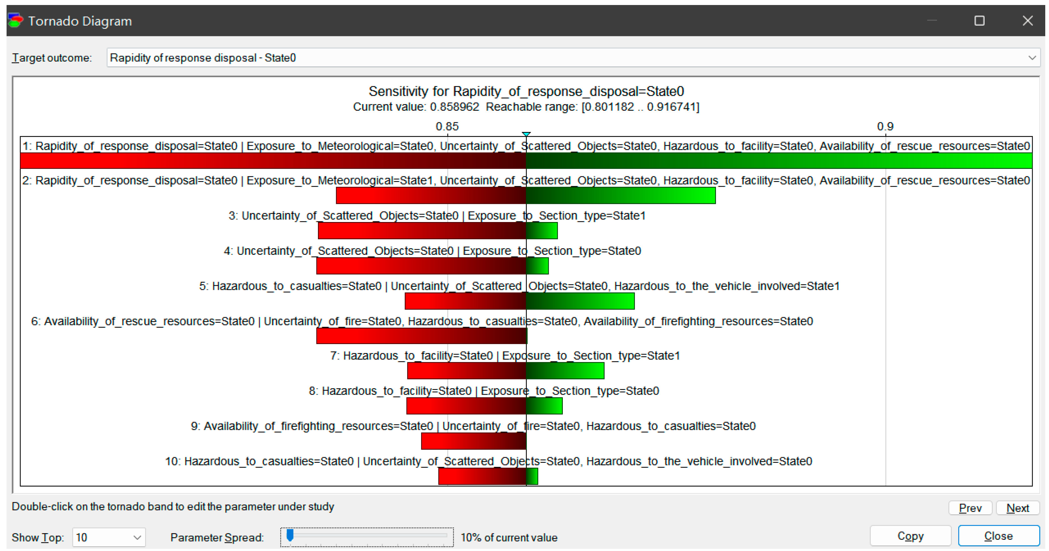
5.3. Resilience Evolution Analysis

According to the DBN network structure and network parameters constructed in the previous text, the results of calculating the evolution of road operational resilience are shown in Figure 16. The road’s operational resilience in time slices 0–1 is affected by pressure disturbances and shows a downward trend. In time slices 1–3, the road relies on its physical and topological properties and emergency response disposal to restore resilience to normal levels. In time slices 3–5, resilience returns to normal levels. The integration of resilience inference results into the road operational resilience cube is shown in Figure 17.

This paper employed the 10-fold cross-validation method to evaluate the accuracy of the model. The main idea is to randomly divide the original data into ten subsets of equal size, with nine subsets used for training the model and the remaining one for testing. This process was repeated ten times, with each subset serving as the test set once, and the evaluation results were averaged over the ten rounds. In the model validation process, the road operation resilience result nodes from each time step were taken as the target nodes for model prediction. The overall prediction accuracy, prediction accuracy of each node status, AUC (Area Under the Curve) metric, and ROC (Receiver Operating Characteristic curve) curve were output and used to evaluate the model’s performance.

The Dynamic Bayesian Network model constructed in this paper was found to have high prediction accuracy, with an overall accuracy of 92.19% for the road operation resilience nodes across five time steps. The specific accuracies are shown in

Table 10. Accuracy of node status prediction.

Resilience	t = 1	t = 2	t = 3	t = 4	t = 5
Overall accuracy	0.970682	0.933369	0.953092	0.833156	0.918977
The accuracy of State0	0.974576	0.965708	0.992072	0.986154	0.886105
The accuracy of State1	0.966738	0.903292	0.918429	0.752039	0.929019

. The ROC curve is a visualization tool that describes the performance of a binary classifier at different thresholds. The gray diagonal line on the ROC curve represents the performance of a random classifier, with a better classifier corresponding to a higher curve on the left. AUC is often used as an evaluation index, representing the area under the ROC curve. The larger the AUC value, the better the classifier’s performance. The ROC curve in Figure 18 shows the excellent accuracy of the model for the road operation resilience node at t = 1, with AUC values of 0.96 for both State0 and State1.

Sensitivity analysis can measure the degree of influence of nodes on target events and identify factors that significantly impact them. The BN model’s results on critical factor analysis were verified through domain knowledge. After experimental verification, “scattered objects”, “casualties”, and “availability of rescue resources” sensitivity to “Rapidity of response disposal” decreased in turn. The results are shown in Figure 19. Their slight changes would have a significant impact on traffic accident recovery and disposal.

6. Discussion

Resilience evaluation involves multiple factors, and PSR theory is commonly used to analyze the influencing factors in three dimensions: pressure, state, and response. The deterministic methods used to calculate the final resilience based on this theory can capture resilience relatively comprehensively and reflect both positive and negative feedback effects of resilience under pressure disturbances and emergency responses [37,53,54]. However, these studies often use broad statistical data as calculation indicators, making capturing resilience under specific event impacts challenging. In addition, some studies have not fully considered uncertainty in the resilience evaluation process, and there are fewer examinations of correlations between resilience-influencing factors.

In the road traffic field, resilience research mainly constructs models focused on functional changes in roads and relevant variables as resilience attributes [17,18]. However, these models cannot demonstrate the multidimensional effects of pressure disturbances, state resistance, and response recovery that roads face during emergency events. Furthermore, measuring dynamic changes in resilience has been constrained by using static Bayesian networks or rough-grained indicators.

This study proposes a novel road resilience modeling and evaluation method, combining domain knowledge with historical data on emergency events using PSR and DBN theories. Cross-validation and sensitivity analysis verified the model’s accuracy and examined key factors affecting resilience.

However, this paper acknowledges that some limitations of the current method cannot be ignored and that there is room for improving model accuracy and application scenarios. Data quality and accuracy may be improved by strengthening data collection methods, especially for manual text records. A more refined classification of node resilience status could achieve a more precise resilience measurement. Additionally, future work could focus on measuring resilience for a particular type of severe disaster event, such as a hazardous chemical accident, through a more targeted Dynamic Bayesian Network model.

7. Conclusions

This article proposes a new definition for road resilience in terms of operational resilience modeling. It identifies influential factors in different dimensions (pressure, state, and response). It establishes interaction mechanisms between elements, achieving three-stage modeling and integrated visualization for “defensive disturbance, rapid absorption, and immediate recovery” in different dimensions. The article solves the problem of the difficulty of multidimensional resilience modeling.

Regarding the quantification of road resilience, the article proposes a layered DBN network structure based on domain knowledge, describing the dependence relationships and dynamic features of multidimensional factors affecting road resilience. Using BWM and D–S evidence theory, the article addresses the issue of incomplete data and complex dependence relationships between resilience factors in DBN node resilience status judgment. It implements a new method for measuring road operational resilience driven by a fusion of domain knowledge and data.

Furthermore, sensitivity analysis using Bayesian networks showed that the key factors affecting the response time are “scattered objects”, “casualties”, and “availability of rescue resources”, which can help managers take targeted measures to enhance road operational resilience.

The methods proposed in this article have been validated and applied to Shanghai’s urban expressway network and will be further promoted by providing more road facilities.

References

1. Ganin, A.A.; Kitsak, M.; Marchese, D.; Keisler, J.M.; Seager, T.; Linkov, I. Resilience and Efficiency in Transportation Networks. Sci. Adv. 2017, 3, e1701079. [Google Scholar] [CrossRef] [PubMed] [Green Version]
2. Climate Change Cost New York $8 Billion During Hurricane Sandy—Bloomberg. Available online: https://www.bloomberg.com/news/articles/2021-05-18/climate-change-cost-new-york-8-billion-during-hurricane-sandy#xj4y7vzkg (accessed on 8 April 2023).
3. National Data. Available online: https://data.stats.gov.cn/easyquery.htm?cn=C01 (accessed on 14 June 2023).
4. Rezvani, S.M.; Falcão, M.J.; Komljenovic, D.; de Almeida, N.M. A Systematic Literature Review on Urban Resilience Enabled with Asset and Disaster Risk Management Approaches and GIS-Based Decision Support Tools. Appl. Sci. 2023, 13, 2223. [Google Scholar] [CrossRef]
5. Murray-Tuite, P. A Comparison of Transportation Network Resilience under Simulated System Optimum and User Equilibrium Conditions. In Proceedings of the 2006 Winter Simulation Conference, Monterey, CA, USA, 3–6 December 2006; IEEE: Monterey, CA, USA; pp. 1398–1405. [Google Scholar]
6. Lounis, Z. Risk-Based Decision Making for Sustainable and Resilient Infrastructure. J. Struct. Eng. 2013, 142, 1845–1856. [Google Scholar] [CrossRef]
7. Zimmerman, R.; Zhu, Q.; de Leon, F.; Guo, Z. Conceptual Modeling Framework to Integrate Resilient and Interdependent Infrastructure in Extreme Weather. J. Infrastruct. Syst. 2017, 23, 04017034. [Google Scholar] [CrossRef]
8. Henry, D.; Emmanuel Ramirez-Marquez, J. Generic Metrics and Quantitative Approaches for System Resilience as a Function of Time. Reliab. Eng. Syst. Saf. 2012, 99, 114–122. [Google Scholar] [CrossRef]
9. Kammouh, O.; Dervishaj, G.; Cimellaro, G.P. A New Resilience Rating System for Countries and States. Procedia Eng. 2017, 198, 985–998. [Google Scholar] [CrossRef] [Green Version]
10. Kammouh, O.; Zamani Noori, A.; Cimellaro, G.P.; Mahin, S.A. Resilience Assessment of Urban Communities. ASCE-ASME J. Risk Uncertain. Eng. Syst. Part A Civ. Eng. 2019, 5, 04019002. [Google Scholar] [CrossRef] [Green Version]
11. De Iuliis, M.; Kammouh, O.; Cimellaro, G.P.; Tesfamariam, S. Downtime Estimation of Building Structures Using Fuzzy Logic. Int. J. Disaster Risk Reduct. 2019, 34, 196–208. [Google Scholar] [CrossRef]
12. Kammouh, O.; Cimellaro, G.P.; Mahin, S.A. Downtime Estimation and Analysis of Lifelines after an Earthquake. Eng. Struct. 2018, 173, 393–403. [Google Scholar] [CrossRef]
13. Kammouh, O.; Noori, A.Z.; Taurino, V.; Mahin, S.A.; Cimellaro, G.P. Deterministic and Fuzzy-Based Methods to Evaluate Community Resilience. Earthq. Eng. Eng. Vib. 2018, 17, 261–275. [Google Scholar] [CrossRef]
14. Dehghani, F.; Mohammadi, M.; Karimi, M. Age-Dependent Resilience Assessment and Quantification of Distribution Systems under Extreme Weather Events. Int. J. Electr. Power Energy Syst. 2023, 150, 109089. [Google Scholar] [CrossRef]
15. Soni, U.; Jain, V.; Kumar, S. Measuring Supply Chain Resilience Using a Deterministic Modeling Approach. Comput. Ind. Eng. 2014, 74, 11–25. [Google Scholar] [CrossRef]
16. Kammouh, O.; Gardoni, P.; Cimellaro, G.P. Probabilistic Framework to Evaluate the Resilience of Engineering Systems Using Bayesian and Dynamic Bayesian Networks. Reliab. Eng. Syst. Saf. 2020, 198, 106813. [Google Scholar] [CrossRef]
17. Tang, J.; Heinimann, H.; Han, K.; Luo, H.; Zhong, B. Evaluating Resilience in Urban Transportation Systems for Sustainability: A Systems-Based Bayesian Network Model. Transp. Res. Part C Emerg. Technol. 2020, 121, 102840. [Google Scholar] [CrossRef]
18. Chen, H.; Zhou, R.; Chen, H.; Lau, A. Static and Dynamic Resilience Assessment for Sustainable Urban Transportation Systems: A Case Study of Xi ’an, China. J. Clean. Prod. 2022, 368, 133237. [Google Scholar] [CrossRef]
19. Zhu, C.; Wu, J.; Liu, M.; Luan, J.; Li, T.; Hu, K. Cyber-Physical Resilience Modelling and Assessment of Urban Roadway System Interrupted by Rainfall. Reliab. Eng. Syst. Saf. 2020, 204, 107095. [Google Scholar] [CrossRef]
20. Jiang, S.; Yang, L.; Cheng, G.; Gao, X.; Feng, T.; Zhou, Y. A Quantitative Framework for Network Resilience Evaluation Using Dynamic Bayesian Network. Comput. Commun. 2022, 194, 387–398. [Google Scholar] [CrossRef]
21. Yang, L.; Li, K.; Song, G.; Khan, F. Dynamic Railway Derailment Risk Analysis with Text-Data-Based Bayesian Network. Appl. Sci. 2021, 11, 994. [Google Scholar] [CrossRef]
22. Tong, Q.; Yang, M.; Zinetullina, A. A Dynamic Bayesian Network-Based Approach to Resilience Assessment of Engineered Systems. J. Loss Prev. Process Ind. 2020, 65, 104152. [Google Scholar] [CrossRef]
23. Sen, M.K.; Dutta, S.; Kabir, G. Modelling and Quantification of Time-Varying Flood Resilience for Housing Infrastructure Using Dynamic Bayesian Network. J. Clean. Prod. 2022, 361, 132266. [Google Scholar] [CrossRef]
24. Zhang, X.; Chen, G.; Yang, D.; He, R.; Zhu, J.; Jiang, S.; Huang, J. A Novel Resilience Modeling Method for Community System Considering Natural Gas Leakage Evolution. Process Saf. Environ. Prot. 2022, 168, 846–857. [Google Scholar] [CrossRef]
25. Wang, J.; Gao, S.; Yu, L.; Ma, C.; Zhang, D.; Kou, L. A Data-Driven Integrated Framework for Predictive Probabilistic Risk Analytics of Overhead Contact Lines Based on Dynamic Bayesian Network. Reliab. Eng. Syst. Saf. 2023, 235, 109266. [Google Scholar] [CrossRef]
26. Vagnoli, M.; Remenyte-Prescott, R. Updating Conditional Probabilities of Bayesian Belief Networks by Merging Expert Knowledge and System Monitoring Data. Autom. Constr. 2022, 140, 104366. [Google Scholar] [CrossRef]
27. Mottahedi, A.; Sereshki, F.; Ataei, M.; Qarahasanlou, A.N.; Barabadi, A. Resilience Estimation of Critical Infrastructure Systems: Application of Expert Judgment. Reliab. Eng. Syst. Saf. 2021, 215, 107849. [Google Scholar] [CrossRef]
28. Hossain, N.U.I.; Jaradat, R.; Hosseini, S.; Marufuzzaman, M.; Buchanan, R.K. A Framework for Modeling and Assessing System Resilience Using a Bayesian Network: A Case Study of an Interdependent Electrical Infrastructure System. Int. J. Crit. Infrastruct. Prot. 2019, 25, 62–83. [Google Scholar] [CrossRef]
29. Sen, M.K.; Dutta, S.; Kabir, G. Development of Flood Resilience Framework for Housing Infrastructure System: Integration of Best-Worst Method with Evidence Theory. J. Clean. Prod. 2021, 290, 125197. [Google Scholar] [CrossRef]
30. Abdrabo, K.I.; Kantoush, S.A.; Esmaiel, A.; Saber, M.; Sumi, T.; Almamari, M.; Elboshy, B.; Ghoniem, S. An Integrated Indicator-Based Approach for Constructing an Urban Flood Vulnerability Index as an Urban Decision-Making Tool Using the PCA and AHP Techniques: A Case Study of Alexandria, Egypt. Urban Clim. 2023, 48, 101426. [Google Scholar] [CrossRef]
31. Liu, D.; Qi, X.; Fu, Q.; Li, M.; Zhu, W.; Zhang, L.; Abrar Faiz, M.; Khan, M.I.; Li, T.; Cui, S. A Resilience Evaluation Method for a Combined Regional Agricultural Water and Soil Resource System Based on Weighted Mahalanobis Distance and a Gray-TOPSIS Model. J. Clean. Prod. 2019, 229, 667–679. [Google Scholar] [CrossRef]
32. Zarei, E.; Ramavandi, B.; Darabi, A.H.; Omidvar, M. A Framework for Resilience Assessment in Process Systems Using a Fuzzy Hybrid MCDM Model. J. Loss Prev. Process Ind. 2021, 69, 104375. [Google Scholar] [CrossRef]
33. Mohammed, A.; Zubairu, N.; Yazdani, M.; Diabat, A.; Li, X. Resilient Supply Chain Network Design without Lagging Sustainability Responsibilities. Appl. Soft Comput. 2023, 140, 110225. [Google Scholar] [CrossRef]
34. Bruneau, M.; Chang, S.E.; Eguchi, R.T.; Lee, G.C.; O’Rourke, T.D.; Reinhorn, A.M.; Shinozuka, M.; Tierney, K.; Wallace, W.A.; von Winterfeldt, D. A Framework to Quantitatively Assess and Enhance the Seismic Resilience of Communities. Earthq. Spectra 2003, 19, 733–752. [Google Scholar] [CrossRef] [Green Version]
35. Hosseini, Y.; Karami Mohammadi, R.; Yang, T.Y. Resource-Based Seismic Resilience Optimization of the Blocked Urban Road Network in Emergency Response Phase Considering Uncertainties. Int. J. Disaster Risk Reduct. 2023, 85, 103496. [Google Scholar] [CrossRef]
36. Chavoshy, A.; Amini Hosseini, K.; Hosseini, M. Resiliency Cube: A New Approach for Parametric Analysis of Earthquake Resiliency in Urban Road Networks. IJDRBE 2018, 9, 317–332. [Google Scholar] [CrossRef]
37. Chen, M.; Jiang, Y.; Wang, E.; Wang, Y.; Zhang, J. Measuring Urban Infrastructure Resilience via Pressure-State-Response Framework in Four Chinese Municipalities. Appl. Sci. 2022, 12, 2819. [Google Scholar] [CrossRef]
38. Ouyang, M.; Dueñas-Osorio, L.; Min, X. A Three-Stage Resilience Analysis Framework for Urban Infrastructure Systems. Struct. Saf. 2012, 36–37, 23–31. [Google Scholar] [CrossRef]
39. Yin, J.; Ren, X.; Liu, R.; Tang, T.; Su, S. Quantitative Analysis for Resilience-Based Urban Rail Systems: A Hybrid Knowledge-Based and Data-Driven Approach. Reliab. Eng. Syst. Saf. 2022, 219, 108183. [Google Scholar] [CrossRef]
40. Sonal; Ghosh, D. Impact of Situational Awareness Attributes for Resilience Assessment of Active Distribution Networks Using Hybrid Dynamic Bayesian Multi Criteria Decision-Making Approach. Reliab. Eng. Syst. Saf. 2022, 228, 108772. [Google Scholar] [CrossRef]
41. Tien, I. Theoretical Systems Modeling Framework for Sustainability Using Bayesian and Dynamic Bayesian Networks. In Reference Module in Earth Systems and Environmental Sciences; Elsevier: Amsterdam, The Netherlands, 2023; ISBN 978-0-12-409548-9. [Google Scholar]
42. GA/T 16.1-16.18-2010; Codes for traffic accident information. Standard Press of China: Beijing, China, 2010.
43. GA 17.1-17.11-2003; Codes for Road Traffic Accident Scene. Standard Press of China: Beijing, China, 2003.
44. Barry, D.J. Estimating Runway Veer-off Risk Using a Bayesian Network with Flight Data. Transp. Res. Part C Emerg. Technol. 2021, 128, 103180. [Google Scholar] [CrossRef]
45. Karimnezhad, A.; Moradi, F. Road Accident Data Analysis Using Bayesian Networks. Transp. Lett. 2017, 9, 12–19. [Google Scholar] [CrossRef]
46. Rezaei, J. Best-Worst Multi-Criteria Decision-Making Method: Some Properties and a Linear Model. Omega 2016, 64, 126–130. [Google Scholar] [CrossRef]
47. Rezaei, J.; Nispeling, T.; Sarkis, J.; Tavasszy, L. A Supplier Selection Life Cycle Approach Integrating Traditional and Environmental Criteria Using the Best Worst Method. J. Clean. Prod. 2016, 135, 577–588. [Google Scholar] [CrossRef]
48. Ballent, W.; Corotis, R.B.; Torres-Machi, C. Representing Uncertainty in Natural Hazard Risk Assessment with Dempster Shafer (Evidence) Theory. Sustain. Resilient Infrastruct. 2019, 4, 137–151. [Google Scholar] [CrossRef]
49. Attoh-Okine, N.O.; Cooper, A.T.; Mensah, S.A. Formulation of Resilience Index of Urban Infrastructure Using Belief Functions. IEEE Syst. J. 2009, 3, 147–153. [Google Scholar] [CrossRef]
50. Nair, S.; Walkinshaw, N.; Kelly, T.; de la Vara, J.L. An Evidential Reasoning Approach for Assessing Confidence in Safety Evidence. In Proceedings of the 2015 IEEE 26th International Symposium on Software Reliability Engineering (ISSRE), Gaithersbury, MD, USA, 2–5 November 2015; pp. 541–552. [Google Scholar]
51. Huang, W.; Kou, X.; Zhang, Y.; Mi, R.; Yin, D.; Xiao, W.; Liu, Z. Operational Failure Analysis of High-Speed Electric Multiple Units: A Bayesian Network-K2 Algorithm-Expectation Maximization Approach. Reliab. Eng. Syst. Saf. 2021, 205, 107250. [Google Scholar] [CrossRef]
52. GeNIe Modeler. Available online: https://support.bayesfusion.com/docs/GeNIe/ (accessed on 8 April 2023).
53. Jiao, L.; Wang, L.; Lu, H.; Fan, Y.; Zhang, Y.; Wu, Y. An Assessment Model for Urban Resilience Based on the Pressure-State-Response Framework and BP-GA Neural Network. Urban Clim. 2023, 49, 101543. [Google Scholar] [CrossRef]
54. Zheng, J.; Huang, G. Towards Flood Risk Reduction: Commonalities and Differences between Urban Flood Resilience and Risk Based on a Case Study in the Pearl River Delta. Int. J. Disaster Risk Reduct. 2023, 86, 103568. [Google Scholar] [CrossRef]
Figure 1. Hierarchical framework of road operational resilience elements based on PSR theory.
Applsci 13 07481 g001
Figure 2. Mechanisms of road operational resilience elements. (The light red color in the chart related to pressure resilience. The light green color in the chart related to state resilience. The light blue color in the chart elated to response resilience).
Applsci 13 07481 g002
Figure 3. Bayesian network structure based on the hierarchical framework of road operational resilience elements.
Applsci 13 07481 g003
Figure 4. Bayesian network structure taking into account node relationships across different time slices.
Applsci 13 07481 g004
Figure 5. Unrolled DBN structure.
Applsci 13 07481 g005
Figure 6. DBN structure with improved factor correlation on road operational resilience. The dashed borders represent pending relationships between nodes, while the solid borders represent confirmed relationships between nodes.
Applsci 13 07481 g006
Figure 7. DBN of road operational resilience considering the time characteristics of the elements.
Applsci 13 07481 g007
Figure 8. D–S + BWM process for judging node resilience status in Bayesian networks among different levels.
Applsci 13 07481 g008
Figure 9. Road operational resilience cube at the 0 T 1 moment. The red spatial geometric bodies represent resilience to pressure, the green spatial geometric bodies represent resilience to states, and the blue spatial geometric bodies represent resilience to responses.
Applsci 13 07481 g009
Figure 10. Evolution of the road operational resilience cube based on PSR. Figure (ac): Road Operational Resilience Cube for Time Intervals T0-T1, T0-T2, T0-T3.
Applsci 13 07481 g010
Figure 11. Integration and visualization of multidimensional resilience. Figure (ac) respectively represent the x-z plane projection, y-z plane cross-section, and x-y plane projection.
Applsci 13 07481 g011
Figure 12. Initial hierarchical Bayesian network structure in GeNie.
Applsci 13 07481 g012
Figure 13. Bayesian Network Structure considering node relationships between time slices in GeNie.
Applsci 13 07481 g013
Figure 14. Dynamic Bayesian Network structure of the hierarchical road operational resilience in GeNie.
Applsci 13 07481 g014
Figure 15. Conditional probability table of road operational resilience.
Applsci 13 07481 g015
Figure 16. Evolution results of road operational resilience on the Shanghai expressway.
Applsci 13 07481 g016
Figure 17. Road operational resilience cube of the Shanghai expressway. Figure (ac) respectively represent the x-z plane projection, y-z plane cross-section, and x-y plane projection.
Applsci 13 07481 g017
Figure 18. ROC curve of node resilience at t = 1.
Applsci 13 07481 g018
Figure 19. Sensitivity analysis results. The color of the bar shows the direction of the change in the target state, red expresses negative and green positive change.
Applsci 13 07481 g019