
Study on Dynamic Uncertainty and Sensitivity of Gear System Considering the Influence of Machining Accuracy

1
Key Laboratory of Road Construction Technology and Equipment of Ministry of Education, Chang′an University, Middle-Section of Nan′er Huan Road, Xi′an 710064, China
2
School of Construction Machinery, Chang′an University, Middle-Section of Nan′er Huan Road, Xi′an 710064, China
3
School of Mechanical and Precision Instrument Engineering, Xi′an University of Technology, No.5 South Jinhua Road, Xi′an 710048, China
*
Author to whom correspondence should be addressed.
Appl. Sci. 2023, 13(14), 8011; https://doi.org/10.3390/app13148011
Submission received: 12 June 2023
/
Revised: 4 July 2023
/
Accepted: 6 July 2023
/
Published: 8 July 2023
Abstract
:Due to the limitation of machining accuracy, the transmission performance uncertainty of mass gears must be evaluated quantitatively to provide the basis for its application in the whole machine. Based on the polynomial chaotic expansion (PCE) method, a dynamic uncertainty analysis method for gear systems with a specified precision was proposed in this paper. Combined with tooth surface contact analysis and load-bearing contact analysis, a dynamic model of the gear system was established to fully reflect the influence of typical manufacturing errors. Based on this, a PCE model was established to approximate the system dynamics model. The dynamic uncertainty of the gear system was quantified based on the PCE approximation model and the Monte Carlo method, respectively, and the computational accuracy and efficiency of the PCE model with different orders and numbers of sample points were compared and analyzed. Finally, Sobol′ sensitivity indices from the PCE model of the gear system to random errors were computed, and the primary and secondary relationships of influence on the dynamic performance of the gear system were determined. The results showed that the PCE method had good applicability to the quantification of dynamic uncertainty and error sensitivity analysis of gear systems, and it had both accuracy and high efficiency.
1. Introduction
Gear transmission has been widely used in aircrafts, ships, automobiles, wind turbines, excavators, and so on. With the above mechanical equipment entering the development stage of high speed, high precision, and high reliability, the dynamic performance and transmission reliability of gear transmission are facing higher demands. However, in practical engineering, uncertain factors exist widely in machine tools, cutting tools, and machining motions, so gear machining errors are inevitable and uncertain. The sensitivity of gear transmission performance to random error enlarges the gap between the expected design goal and the practical application effect and affects the feasibility of the gear design scheme and the consistency of gear transmission performance in the batch. Therefore, it is necessary to study the influence of the law of random errors on the dynamic performance of gear systems and observe the error sensitivity of the system dynamic performance when the working conditions change.
The influence of machining error and its randomness has been studied in the design and analysis of gear transmission. Donmez and Kahraman [1] predicted the gear rattle when considering the eccentricities and tooth indexing errors, and it was proved by experiments that such errors are likely to increase the gear rattle severity. Zhang et al. [2] derived the similarity relationship of a gear system when considering the machining error and proposed two modification methods for the scale model prediction to solve machining error distortion. Zhou et al. [3] proposed a crack initiation life model of standard and error gears in accordance with tooth stress history and a critical plane method for non-proportional loading and investigated the effects of centering error and angular misalignment on crack initiation life in herringbone gears. Vivet et al. [4] performed tooth contact analysis of spiral bevel gears to investigate the simulation of gear alignment errors. Some studies revealed the influence of machining accuracy on gear transmission performance. Bonori and Pellicano [5] treated the profile error as a random variable and analyzed the effects of profile errors and their variances on the gear vibration. Driot and Perret-Liaudet [6] predicted the variability of the dynamic behavior of a gear pair system due to tolerances. Liu et al. [7] predicted the range of the transmission error for the spur gear pair under different grades. Guo and Fang [8] performed a statistical analysis on the effect of random manufacturing errors on the system′s dynamic performance of the gears under different accuracy grades. Some other scholars have studied the uncertainty propagation of errors and the impact on system reliability. Thomas et al. [9] proposed a surrogate model-based uncertainty quantification and studied the uncertainty propagations of the shaft deviations and tooth surface deviations in a helical gear pair by using the model. Chen et al. [10] analyzed the sensitivities of random gear parameters to the wind turbine gear system reliability. The randomness of errors indeed leads to the uncertainty of the dynamic transmission of the system. When changing operating parameters, such as torque or speed, the uncertainty may be aggravated. Therefore, it is of great significance to predict the dynamic behaviors of gear systems with random errors efficiently and accurately to reveal the influence mechanism of random errors under multiple working conditions.
In the research of dynamic uncertain behaviors of gear systems, two uncertain analysis methods of probability and interval are mainly used. Bel Mabrouk et al. [11] analyzed the dynamic behavior of a bevel gear system with uncertainty parameters based on the projection of polynomial chaos. Kahnamouei and Yang [12] analyzed the nonlinear stochastic vibration of a wind turbine′s planetary gear train by using the statistical linearization technique. Zhang and Guo [13] presented the modification uncertainty analysis of helical planetary gears by using the response surface method and Monte Carlo simulation. Hu et al. [14] investigated error randomness in the dynamic load-sharing behavior of the closed differential planetary transmission system, based on the Monte Carlo method. Liu et al. [15] established the probability distribution models of gear time-varying meshing stiffness with the random pitting of tooth surfaces and verified the model using the Monte Carlo method. Wei et al. [16] investigated the dynamic responses of a geared transmission system with uncertain parameters, based on the Chebyshev interval method. Xun et al. [17] analyzed the statistical property of the dynamic performance of planetary gear trains, based on the method of multiple scales. In the above studies, Monte Carlo simulation is most commonly used, but it is computationally intensive and inefficient. Polynomial chaotic expansion and the response surface method belong to the proxy model method of probabilistic method, which have low computation and high efficiency. In particular, the polynomial chaotic expansion method has been widely used [18,19,20]. The interval method can only give the variation range of the output response of the system but cannot obtain its statistical rule.
In this work, the polynomial chaotic expansion (PCE) method was applied to the dynamic uncertainty analysis of gear systems to consider stochastic errors, and the Monte Carlo method was used to verify the effectiveness of this method. The sensitivity indices of the gear system to random errors were calculated based on the PCE model. This study provides reference and support for dynamic performance evaluation and the optimal design of the gear transmission system.
2. The Original Dynamic Model of Gear System
In this section, the influence of typical manufacturing errors is reasonably introduced into the gear system dynamic model, based on actual tooth surface contact analysis. The static meshing simulation of a gear pair with manufacturing errors is carried out (see Section 2.1). The main internal excitations of the transmission error, time-varying meshing stiffness, and meshing-in impact are calculated, based on the meshing performance while considering the influence of errors (see Section 2.2). Finally, the dynamic equation of the gear system incorporating transmission error excitation, time-varying meshing stiffness, and meshing-in impact is derived, as can be seen in Section 2.3. The mapping relationship between the error sample and the system output response is established throughout the whole process.
2.1. Actual Tooth Surface Contact Analysis
2.1.1. Mathematical Modeling of Typical Manufacturing Errors
In this paper, four kinds of typical manufacturing errors were selected, including shape deviation and slope deviation along the directions of the tooth profile and the lead, respectively shown in Figure 1. These errors were defined, and the limit deviation corresponding to the machining accuracy was given in the standard of ISO 1328-1:2013 [21].
The common shape deviation mainly included three forms, concave, convex, and wavy, shown in Figure 2. Among them, the wavy deviation was mainly caused by the vibration during processing or the low-hardness tooth surface scuffing. Generally, its value was small and irregular, which had little influence on the performance of gear transmission. Therefore, this paper mainly considered two forms of concave and convex. The shape deviations along the directions of the tooth profile and the lead, respectively, were simulated by the semi-sine function shown in Equations (1) and (2).
where δfα is the shape deviation of tooth profile, δfβ is the shape deviation of the lead, and Efα and Efβ are the amplitudes of the shape deviation determined by random sampling, according to the gear precision grade; the determination of the parameters h1, h2, l1, and l2 are shown in Figure 3. In this figure, the origin o of the coordinate system oxyz is the rotation center of the gear, plane oxy is parallel to the end of the gear, h1 and h2 are the radii of the root and top for the working tooth surface, l1 and l2 are the coordinate values projected on the z-axis at both ends of the lead, H is the working tooth height projected onto the axial section, and B is the tooth width.
The slope deviation had different directions, as shown in Figure 4. Due to the change in the direction of the slope deviation, the root or top protruded along the direction of the tooth profile, and one of the two ends protruded along the direction of the lead. The formula of the slope deviation in each direction is also specified in Equation (3).
where δHα is the slope deviation of the tooth profile, δHβ is the slope deviation of the lead, and EHα and EHβ are the amplitudes of the slope deviation determined by random sampling according to the gear precision grade.
2.1.2. Meshing Performance Analysis of Actual Tooth Surface
The actual tooth surface was constructed by the superposition of the theoretical tooth surface and normal deviation surface. As shown in Figure 5, mesh was divided on the tooth surface. The position vector r0 (x, y, z) of point N on the theoretical tooth surface was obtained, based on the space meshing theory [22,23]. The tooth surface deviation, δ(h, l), corresponding to point N was calculated by the mathematical model of each error. The corresponding relationship between coordinates of the theoretical tooth surface and the deviation surface is shown in Equation (4). Based on the superposition of the deviation δ and the position vector r0 of the theoretical tooth surface, the position vector and normal vector of the actual tooth surface are expressed in Equations (5) and (6).
where u and θ are the parameters of the tooth surface, and the relationships between them and tooth surface coordinates x, y, and z are shown in reference [23]. n0 is the unit normal vector of the theoretical tooth surface.
A pair of helix gears was used as an example, whose parameters are shown in Table 1. The value of each error was randomly sampled within the tolerance limit of level 5, as shown in Table 2. In order to better analyze the influence of error, only the tooth surface error of the pinion was considered in this paper. Tooth contact analysis (TCA) and loaded tooth contact analysis (LTCA) were carried out based on the actual tooth surface.
Figure 6 shows the loaded transmission error (LTE) and the unloaded transmission error (TE) of the helical gear pair with errors. TE is mainly caused by the gap between the teeth. LTE includes the gap between the teeth and the bearing deformation of the tooth surface. The influence of errors on the gear meshing performance was analyzed by comparing them with a case with no errors. Figure 7 illustrates the amplitude of LTE and the load distribution of the tooth surface for the two cases. It can be seen from Figure 7 that due to the existence of errors, the amplitude of LTE increased significantly, and the phenomenon of uneven load-bearing on the tooth surface occurred. These effects were not conducive to the smooth operation of gears.
2.2. Internal Excitation Calculation Based on Actual Meshing Performance
The dynamic model in this paper mainly considered three kinds of excitation, namely static transmission error, time-varying meshing stiffness, and meshing-in impact. TE was regarded as the static transmission error. The calculations of the other two kinds of excitation are mainly introduced below.
2.2.1. Determination of Time-Varying Mesh Stiffness
The time-varying mesh stiffness refers to the ability of all tooth pairs engaged at the same time to resist the elastic deformation of the tooth in the process of gear transmission. Based on this, the calculation formula is given in Equation (7).
where Fn is the normal force on the tooth surface, and dn is the comprehensive deformation of simultaneous meshing tooth pairs, which can be calculated by Equation (8).
where δLTE and δTE are, respectively, LTE and TE along the line of action.
Based on Equations (7) and (8), the time-varying mesh stiffness was calculated, as shown in Figure 8.
2.2.2. Meshing-In Impact
Under the load condition shown in Table 1, the gear pair had full tooth surface contact, so the initial engagement occurred at the tip of the gear and the tooth surface of the pinion. However, due to the concave form error and slope error shown by the yellow line in Figure 4 defined in this paper, the meshing-in end of the pinion protruded. On the contrary, the convex form error and the slope error shown by the blue line in Figure 4 made the meshing-out end of the pinion protrude. The time and position of meshing-in interference outside the theoretical line of action were different in these two cases. Therefore, two methods for calculating the meshing-in impact were proposed for the two cases above.
Figure 9 shows the actual initial meshing positions in the two cases above. Point D was the theoretical meshing-in point on the theoretical line of action, N1N2, without considering the manufacturing error and the deformation of the tooth surface. Point D0′ was the position of meshing-in interference on the standard surface of the pinion, and point A was the tip of the gear. However, when the meshing-in end of the pinion protruded, as shown in Figure 9a, the meshing-in interference would occur much sooner, which was the actual meshing-in point D′ on the instantaneous line of action, N1′N2′. When the meshing-out end of the pinion protruded, as shown in Figure 9b, there was still a certain gap at the position D0′ between the tooth surface and the tip of the gear. As the gear pair continued to rotate, the meshing-in interference finally occurred at the actual meshing-in point D′.
For the case of the meshing-in end protruding, the accurate position of interference point D′ was determined according to the meshing principle and geometric relation. In Figure 10, point D is the theoretical meshing-in point, and point D′ is the position of the meshing-in interference. Point E is the reverse rotation of point D.
In ∆O1D′O2 and ∆PD′O2:
where
In addition, the basic properties of the involute equation can be calculated by
By combining Equation (9) with Equation (15), the position of the actual meshing-in point D′ could be obtained. In the preceding formula and Figure 10, r1 and r2 are the pitch radii of the pinion and gear, rb1 and rb2 are the base radii of the pinion and gear, ra2 is the tip radius of the gear, φ1 and φ2 are the reverse rotation angles of the pinion and gear, αt is the transverse pressure angle, θLTE is the loaded transmission error of point D′, and i is the transmission ratio.
For the case of the meshing-out end protruding, the meshing position was obtained by tooth contact analysis (TCA). Figure 11 shows the load-distributing factor during the meshing process of a pair of teeth. Due to the concave form error and slope error shown by the blue line in Figure 4, the six points in the blue-dotted box were not in contact and not loaded. Thus, the first point whose load distribution coefficient was not zero was selected as the actual original meshing position, as shown in Figure 11.
The calculations of the impact speed and the stiffness at the initial meshing-in position was introduced in detail by Wu et al. [24] and Guo et al. [25] for the above two cases. Based on the above analysis and the formulas in these literatures, the meshing-in impact was calculated, as shown in Figure 12.
2.3. Dynamic Model of the System
Considering static transmission error, time-varying meshing stiffness, and meshing-in impact, the dynamics model of the gear system was established by using the centralized mass method. Some principles of treatment needed to be adopted. Both gears were treated as rigid discs with radial, axial, and torsional degrees of freedom. Internal excitations of the system acted on the tooth surface along the line of action. The support from the bearings and the shaft was equivalent to the spring fastened to the foundation. The effect of the friction was not taken into account. Based on these principles, the lumped-parameter dynamic model was constructed, as shown in Figure 13.
Based on the established model above, the displacement vector and the relative displacement of the system are listed in Equations (16) and (17).
X = [x1 y1 z1 u1 x2 y2 z2 u2]T
Utilizing the Lagrange equation, the dynamic equations of the system are listed as follows:
where mi and Ii (i = 1, 2) are the mass and rotary inertias of the pinion and gear; Csxi, Csyi, and Cszi and Ksxi, Ksyi, and Kszi (i = 1, 2) are the supporting damping and supporting stiffnesses; Km is the time-varying mesh stiffness; Cm is the mesh damping; Fs is the meshing-in impact; and rb1 and rb2 are the base radii of the pinion and gear.
3. Polynomial Chaos Expansion (PCE) for the Gear System with Random Error
It can be seen from the analysis in Section 2 that the dynamic analysis process of the gear system with manufacturing errors was a complex black-box model, which cannot be described by simple mathematical expressions. The dynamic uncertainty analysis of the gear system based on Monte Carlo simulation requires a large number of samples, and high-precision simulation is costly. Therefore, an efficient and high-precision polynomial chaotic expansion method was used to quantify the dynamic uncertainty of the gear system while considering the randomness of manufacturing errors.
3.1. Random Variable and Its Distribution Model
This paper used four typical manufacturing errors introduced in Section 2.1.1 as random variables. According to the numerical model of these errors and the differentiation of their forms or directions, it was assumed that the errors obeyed the normal distribution, as Ei~(0, σi2) (i = fα, fβ, Hα, Hβ). The standard deviation of the probability distribution model was determined according to the tolerance limit of the gear, as shown in Equation (20).
where Ti is the tolerance limit for the specific precision grade. At this point, the probability that the error sample value exceeded the tolerance limit was only 0.07%.
3.2. Polynomial Chaos Expansion (PCE)
In general, the polynomial chaos theory is an approximate, accurate representation of a random expansion process by the sum of a series of orthogonal polynomials corresponding to the distribution type of the input parameters. In this section, a polynomial chaotic expansion (PCE) model was established for the dynamic uncertainty of the gear system while considering the error randomness. Figure 14 presents the specific flow of the PCE model. In detail, the stochastic dynamic analysis of the gear system was carried out based on the PCE model according to the probability characteristics of the manufacturing error E. For the Gaussian random process, the PCE model could be established by using the Hermit polynomial. The coefficient a of the PCE model was determined by the regression method. In the process of coefficient solving, the selection and combination of N sampling points were crucial, and the corresponding output response should be calculated based on the black-box system model, as shown in Figure 14b.
3.2.1. Determination of Orthogonal Polynomial Base
For the error variables considered in this paper, a four-dimensional parametric polynomial expansion modeling was carried out. The truncation order p was selected as 2 and 3. According to Wiener polynomial chaos, the expressions of two-order and three-order PCEs are shown in Equations (21) and (22).
where ξ = {ξ1, ……, ξd} are the random variables that obey the standard normal distribution and correspond to the error variable E. a = {a0, ai, ……} are the coefficients of PCE, which need to be solved.
3.2.2. The Solution of Polynomial Chaos Expansion Coefficient
The determination of the coefficients is the key step. This paper estimated the coefficient by solving the least square problem [26,27]. Specific steps were described in detail in literatures [26,27], and this paper only listed the linear regression equation, as shown in Equation (23).
where M is the number of the coefficient, with , in which p is the order, and d is the number of random variables; ξ(1), ξ(2), …, ξ(N) are the sample sets of random errors; N is the sample size needed to determine the coefficient, which is usually set as N = 2M, at least for multidimensional uncertainty problems; and y(ξ)(1), y (ξ)(2), …, y (ξ)(N) are the corresponding sets of system responses.
3.3. Precision Analysis of Polynomial Chaotic Expansion Model
In order to effectively compare the accuracy and computational efficiency of PCE models of different orders, this paper dosed a random sampling based on the original system model and the PCE model and solved the dynamic uncertain response of the system by using the Monte Carlo simulation (MCS) and the PCE method, as shown in Figure 15. Due to the limitation of calculation time, the sample size was set at 1000. In the figure, the red curve is the dynamic meshing force of the system without considering the random disturbance of error. The black curves are the system response results of 1000 samples, based on the MCS method. The blue curves in Figure 15a,b are, respectively, the system response results of 1000 samples based on the two-order PCE model, with N = 30 and N = 60. The blue curves in Figure 15c,d are, respectively, the system response results of 1000 samples based on the three-order PCE model, with N = 70 and N = 140. It can be seen that when the number of samples needed to determine the PCE coefficient was set as N = 4M, the calculation accuracy was significantly improved, compared with N = 2M for the two-order or three-order PCE model.
In order to make a more intuitive comparison, this paper further calculated the mean value and standard deviation of the peak-to-peak value of the dynamic meshing force (shown in Table 3) and the relative error (shown in Figure 16) for the two methods. It is worth noting that the computing time shown in the table is the time when four-core parallel computing was adopted, and the calculation time of the PCE model was mainly consumed by solving the PCE coefficient. It can be seen intuitively from Table 3 and Figure 16 that when N = 4M, the mean values obtained by the two-order and three-order PCE models were basically consistent with the calculated results of the MCS method, and the relative errors were both less than 1%. However, for the standard deviation, only the relative error between the three-order PCE model with N = 4M and the MCS method was less than 2%. By comparing the accuracy and calculation time, this paper used the three-order PCE model (N = 4M) to analyze the dynamic uncertainty of the gear system under the influence of random error.
4. Error Sensitivity Analysis of the Dynamic Performance Based on the PCE Model of the Gear System
4.1. Global Sensitivity Analysis Method
Global sensitivity analysis is based on the probability distribution of parameters, and all parameters can change simultaneously during analysis. A quantitative method for global parameter sensitivity analysis was proposed, based on I.M. Sobol in 1990. In this method, the interaction between parameters is considered comprehensively when the sensitivity index of a single parameter is analyzed. The main calculation steps are as follows.
First, all parameters are randomly sampled 2N times to obtain two groups of sample matrices A and B. Then, the sample matrix is obtained by replacing the ith column of matrix A with the ith column of matrix B without changing the other columns. Similarly, the sample matrix is obtained by replacing the ith column of matrix B with the ith column of matrix A without changing the other columns. Based on the PCE model, the corresponding output response value of the sample matrix is calculated.
Second, calculate the variance of the system output corresponding to the sample matrix A.
Calculate the effect of parameter xi on the variance of the system output.
Calculate the effect of parameters other than xi on the variance of the system output.
Finally, the first and total order indices of variable xi are calculated.
4.2. Sensitivity Analysis of System Dynamic Response to Random Manufacturing Errors
By random sampling 20,000 times, the global sensitivities of four typical manufacturing errors to the system dynamic response were analyzed by using the Sobol′ analysis method. The changes in sensitivity indices of each variable were compared by sampling in 5-, 6-, and 7-grade processing accuracies.
The error sensitivity results of the gear system under different precisions are shown in Figure 17. In the figure, the red part is the main effect coefficient, while the white part is the total effect coefficient. It can be seen that the profile shape error had the greatest influence on the peak-to-peak value of the dynamic meshing force, followed by the shape error and slope error along the direction of the lead, and the profile slope error had the least influence. When the machining accuracy of the gear decreased, and the variation range of error expanded, the influence degree of the shape error and slope error along the direction of the lead increased gradually, forming three main influencing factors together with the profile shape error. The influence of the profile slope error was always minimal.
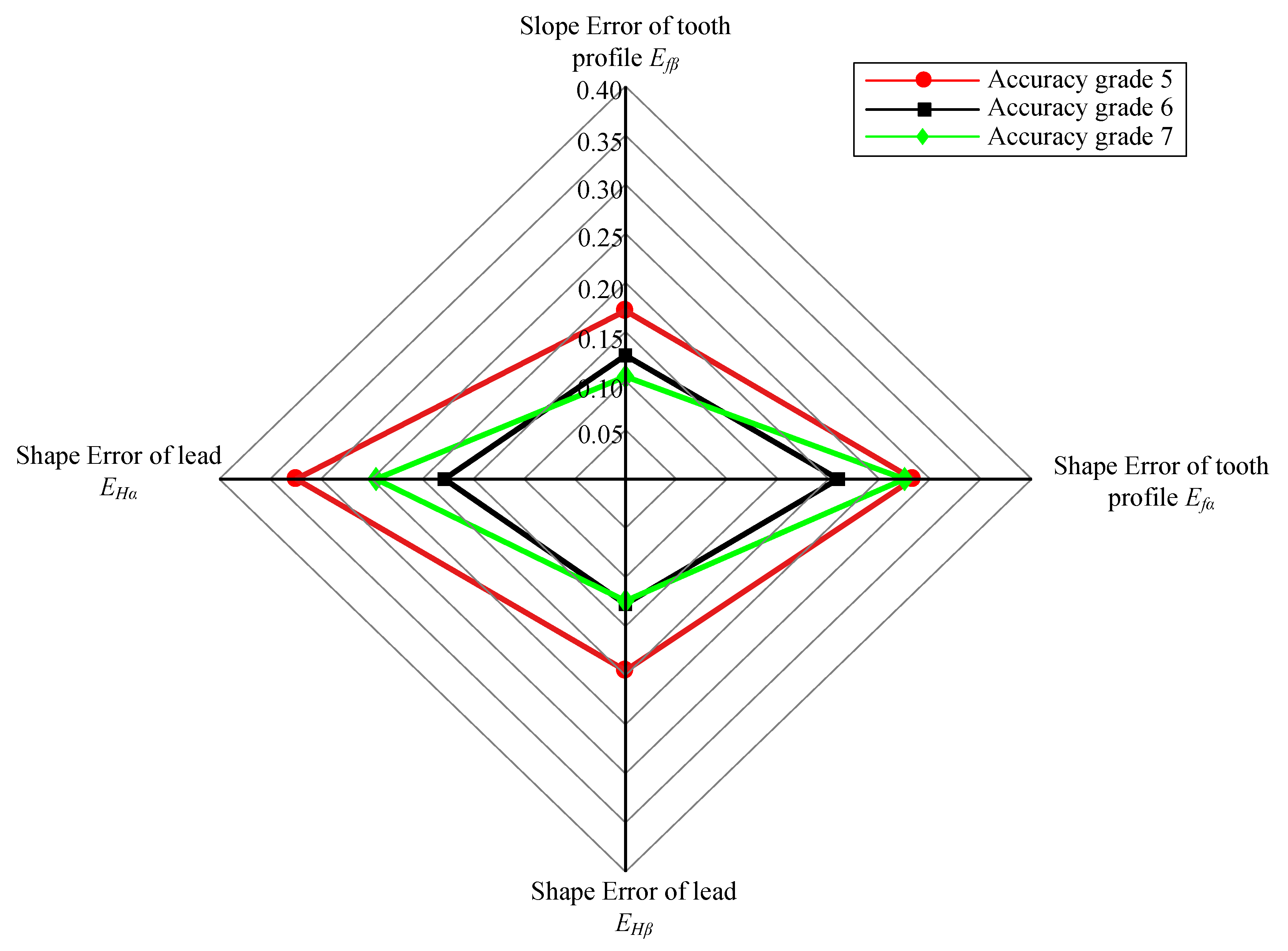
As can be seen from the error sensitivity results above, the main effect coefficients of all errors were smaller than the total effect coefficients, and the differences between them reflect the proportion of the high-order effect of the error. The total interaction effect between each error and other errors is shown in Table 4 and Figure 18. The total interaction effect between the shape error and other errors was greater than that between the slope error and other errors for the three accuracy levels. Compared with grade 5 accuracy, the total interaction effect between each error and other errors was significantly reduced for grade 6 accuracy. The total interaction effect between shape errors and other errors increased obviously when the gear precision grade was changed from 6 to 7.
Through the comparative analysis above, it can be seen that the four typical manufacturing errors had an impact on the dynamic performance of the gear system. Gear precision significantly changes the degree of influence and interaction of each error. In the actual machining of the batch gears, the measurement items of the machined tooth surface can be selected according to the machining accuracy, so as to effectively control the machining quality and ensure the performance consistency of the batch gears. That is, under grade 5 accuracy, the tooth profile shape deviation is the primary control error. At 6 and 7 levels of accuracy, it is also necessary to pay attention to the deviation of the lead.
5. Conclusions
In this paper, a quantitative analysis method based on the polynomial chaotic expansion (PCE) model was proposed to solve the dynamic uncertainty problem of the gear system while considering the error randomness. The sensitivity indices of gear manufacturing errors were analyzed based on the Sobol′ method and the PCE model. The main conclusions are as follows:
- (1)
- Based on tooth contact analysis (TCA), loaded tooth contact analysis (LTCA), and the system dynamic model, a PCE model with the peak–peak value of the dynamic meshing force as the statistical index of the dynamic response was established. When the polynomial expansion ended at the third order, and the number of sample points was four times the number of polynomial coefficients, the PCE model could not only meet the computational accuracy requirements, it also had high computational efficiency.
- (2)
- The accuracy of the PCE model was compared and verified by using the Monte Carlo method. The results showed that the relative error of the mean of the system response was less than 1%, and the relative error of the standard deviation was less than 2%. When the two methods achieved the same accuracy, the PCE method only called the original system model 140 times, which took 0.4 h. The Monte Carlo method called 1000 times, which took 6 h. The PCE method had a higher efficiency and could provide an efficient and accurate new idea for the quantification of dynamic uncertainty and the reliability design of gear systems.
- (3)
- Based on the PCE model, the Sobol′ index of each error was quickly solved. The influence degree of each error on the dynamic performance of gear systems and the change in the interaction effect between errors were compared and analyzed under different precisions. It provides a reference for the machining precision control in the actual machining and application of batch gears.
Author Contributions
Methodology, F.G.; Validation, F.G.; Formal analysis, F.G.; Resources, J.S.; Data curation, F.G.; Writing—original draft, F.G.; Writing—review & editing, F.G.; Visualization, C.L. (Chen Li); Project administration, F.G.; Methodology, C.L. (Chao Liu); Funding acquisition, C.L. (Chao Liu). All authors have read and agreed to the published version of the manuscript.
Funding
This work was financially supported by the Fundamental Research Funds for the Central Universities, CHD (Grant No. 300102252111) and the National Natural Science Foundation of China (Grant No. 52005402).
Institutional Review Board Statement
Not applicable.
Informed Consent Statement
Not applicable.
Data Availability Statement
Not applicable.
Conflicts of Interest
The authors declare no conflict of interest.
References
- Donmez, A.; Kahraman, A. Influence of various manufacturing errors on gear rattle. Mech. Mach. Theory 2022, 173, 104868. [Google Scholar] [CrossRef]
- Zhang, C.P.; Wei, J.; Peng, B.; Cao, M.F.; Hou, S.S.; Lim, T.C. Investigation of dynamic similarity of gear transmission system considering machining error distortion: Theoretical analysis and experiments. Mech. Mach. Theory 2022, 172, 104803. [Google Scholar] [CrossRef]
- Zhou, C.J.; Ning, L.Y.; Wang, H.Y.; Tang, L.W. Effects of centring error and angular misalignment on crack initiation life in herringbone gears. Eng. Fail. Anal. 2021, 120, 105082. [Google Scholar] [CrossRef]
- Vivet, M.; Tamarozzi, T.; Desmet, W.; Mundo, D. On the modelling of gear alignment errors in the tooth contact analysis of spiral bevel gears. Mech. Mach. Theory 2021, 155, 104065. [Google Scholar] [CrossRef]
- Bonori, G.; Pellicano, F. Non-smooth dynamics of spur gears with manufacturing errors. J. Sound Vib. 2007, 306, 271–283. [Google Scholar] [CrossRef]
- Driot, N.; Perret-Liaudet, J. Variability of modal behavior in terms of critical speeds of a gear pair due to manufacturing errors and shaft misalignments. J. Sound Vib. 2006, 292, 824–843. [Google Scholar] [CrossRef]
- Liu, C.; Shi, W.K.; Curá, F.M.; Mura, A. A novel method to predict static transmission error for spur gear pair based on accuracy grade. J. Cent. South Univ. 2020, 27, 3334–3349. [Google Scholar] [CrossRef]
- Guo, F.; Fang, Z.D. The statistical analysis of the dynamic performance of a gear system considering random manufacturing errors under different levels of machining precision. Proc. Inst. Mech. Eng. Part K J. Multi-Body Dyn. 2020, 234, 3–18. [Google Scholar] [CrossRef]
- Diestmann, T.; Broedling, N.; Götz, B.; Melz, T. Surrogate Model-Based Uncertainty Quantification for a Helical Gear Pair. In ICUME 2021: Uncertainty in Mechanical Engineering; Springer: Cham, Switzerland, 2021; pp. 191–207. [Google Scholar]
- Chen, H.T.; Fan, J.K.; Jing, S.X.; Wang, X.H. Probabilistic design optimization of wind turbine gear transmission system based on dynamic reliability. J. Mech. Sci. Technol. 2019, 33, 579–589. [Google Scholar] [CrossRef]
- Bel Mabrouk, I.; El Hami, A.; Walha, L.; Zghal, B.; Haddar, M. Dynamic response analysis of Vertical Axis Wind Turbine geared transmission system with uncertainty. Eng. Struct. 2017, 139, 170–179. [Google Scholar] [CrossRef]
- Kahnamouei, J.T.; Yang, J. Development and verification of a computationally efficient stochastically linearized planetary gear train model with ring elasticity. Mech. Mach. Theory 2021, 155, 104061. [Google Scholar] [CrossRef]
- Zhang, J.; Guo, F. Statistical modification analysis of helical planetary gears based on response surface method and monte carlo simulation. Chin. J. Mech. Eng. 2015, 28, 1194–1203. [Google Scholar] [CrossRef]
- Hu, C.F.; Geng, G.D.; Spanos, P.D. Stochastic dynamic load-sharing analysis of the closed differential planetary transmission gear system by the Monte Carlo method. Mech. Mach. Theory 2021, 165, 104420. [Google Scholar] [CrossRef]
- Liu, W.Z.; Zhu, R.P.; Zhou, W.G.; Shang, Y.W. Probability distribution model of gear time-varying mesh stiffness with random pitting of tooth surface. Eng. Fail. Anal. 2021, 130, 105782. [Google Scholar] [CrossRef]
- Wei, S.; Zhao, J.S.; Han, Q.K.; Chu, F.L. Dynamic response analysis on torsional vibrations of wind turbine geared transmission system with uncertainty. Renew. Energy 2015, 78, 60–67. [Google Scholar] [CrossRef]
- Xun, C.; Long, X.H.; Hua, H.X. Effects of random tooth profile errors on the dynamic behaviors of planetary gears. J. Sound Vib. 2018, 415, 91–110. [Google Scholar] [CrossRef]
- Zhou, Y.C.; Lu, Z.Z.; Yun, W.Y. Active sparse polynomial chaos expansion for system reliability analysis. Reliab. Eng. Syst. Saf. 2020, 202, 107025. [Google Scholar] [CrossRef]
- Wang, F.; Huang, G.H.; Fan, Y.; Li, Y.P. Development of clustered polynomial chaos expansion model for stochastic hydrological prediction. J. Hydrol. 2021, 595, 126022. [Google Scholar] [CrossRef]
- Xiao, H.J.; Song, T.; Jia, B.H.; Lu, X. Uncertainty analysis of MSD crack propagation based on polynomial chaos expansion. Theor. Appl. Fract. Mech. 2022, 120, 103390. [Google Scholar] [CrossRef]
- ISO 1328-1:2013; Cylindrical Gears—ISO System of Flank Tolerance Classification—Part 1: Definitions and Allowable Values of Deviations Relevant to Flanks of Gear Teeth. 2nd ed. International Organization for Standardization: Geneva, Switzerland, 2013; pp. 1–58.
- Litvin, F.L.; Lu, J.; Townsend, D.P.; Howkins, M. Computerized simulation of meshing of conventional helical involute gears and modification of geometry. Mech. Mach. Theory 1999, 34, 123–147. [Google Scholar] [CrossRef] [Green Version]
- Fang, Z.D. Tooth contact analysis of helical gears with modification. J. Aerosp. Power 1997, 12, 247–250. (In Chinese) [Google Scholar]
- Wu, B.; Yang, S.; Yao, J. Theoretical analysis on meshing impact of involute gears. Mech. Sci. Technol. 2003, 22, 55–57. (In Chinese) [Google Scholar]
- Guo, F.; Fang, Z.D.; Zhang, X.J.; Cui, Y.M. Influence of the eccentric error of star gear on the bifurcation properties of herringbone star gear transmission with floating sun gear. Shock Vib. 2018, 2018, 6014570. [Google Scholar] [CrossRef] [Green Version]
- Xiu, D.B.; Karniadakis, G.E. The WIENER-ASKEY polynomial chaos for stochastic differential equations. SIAM J. Sci. Comput. 2002, 24, 619–644. [Google Scholar] [CrossRef]
- Crestaux, T.; Maître, O.L.; Martinez, J. Polynomial chaos expansion for sensitivity analysis. Reliab. Eng. Syst. Saf. 2009, 94, 1161–1172. [Google Scholar] [CrossRef]
Figure 1.
The typical manufacturing errors: (a) shape deviation and slope deviation along the direction of the tooth profile, and (b) shape deviation and slope deviation along the direction of the lead.
Figure 1.
The typical manufacturing errors: (a) shape deviation and slope deviation along the direction of the tooth profile, and (b) shape deviation and slope deviation along the direction of the lead.
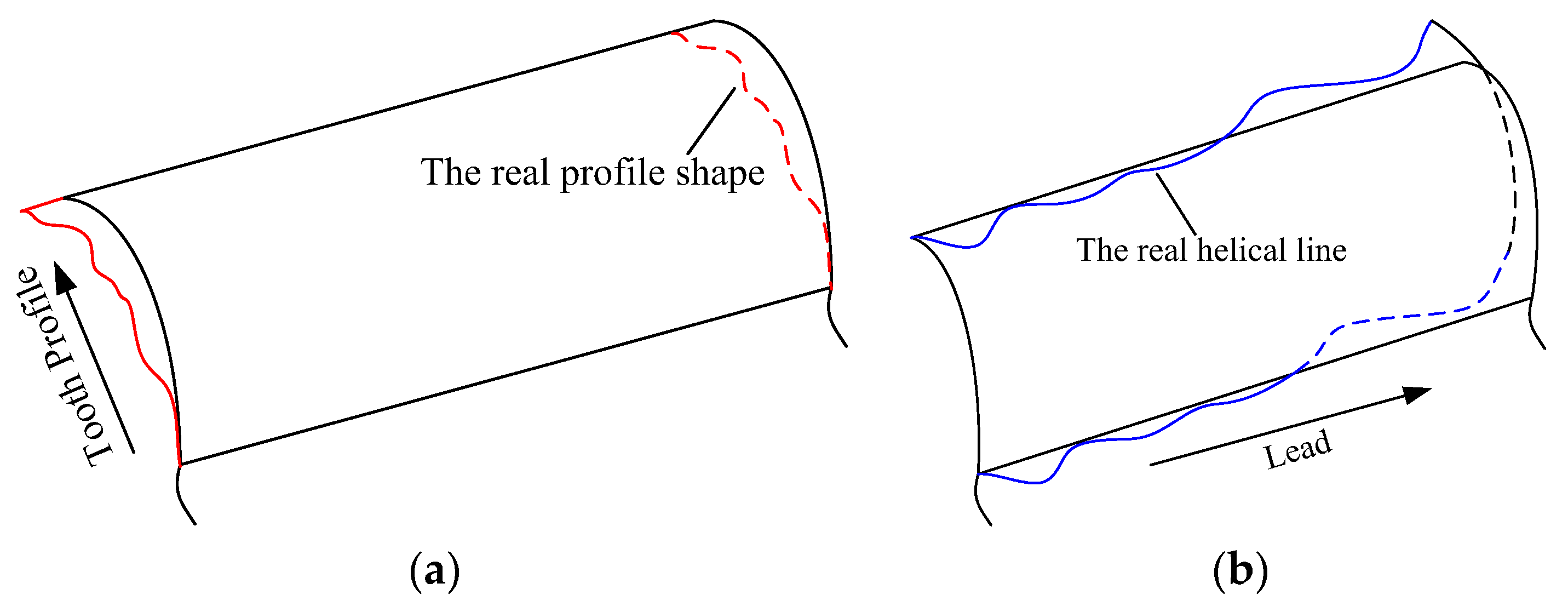
Figure 2.
Three forms of shape deviations in the direction of the tooth profile.
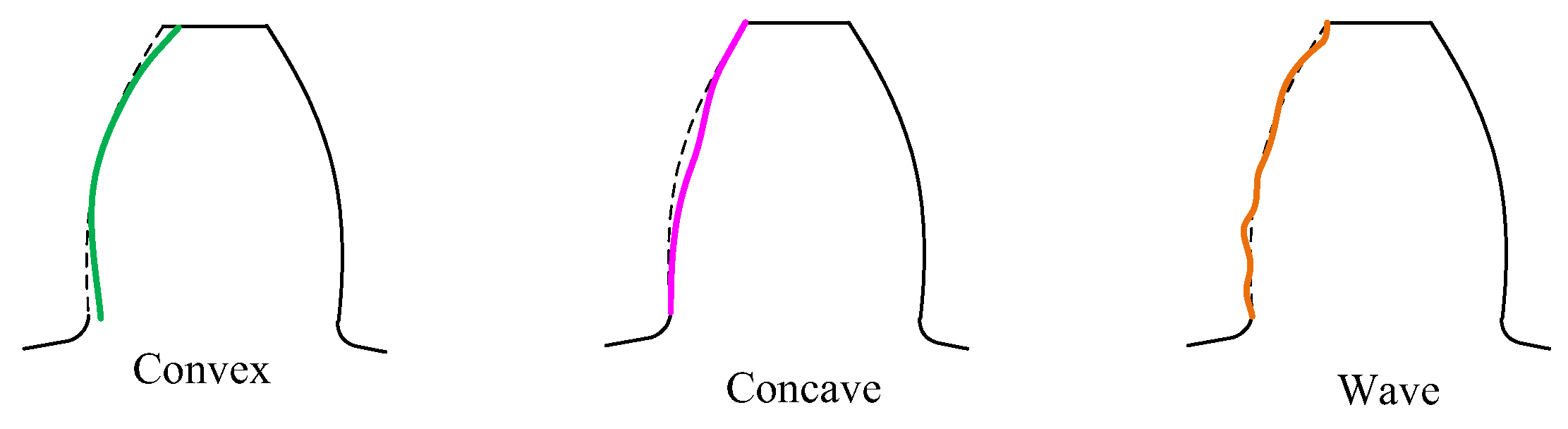
Figure 3.
Description of parameter values in the directions of the tooth profile and tooth width.
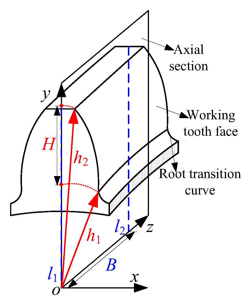
Figure 4.
Different directions of slope errors for the (a) tooth profile and (b) lead.

Figure 5.
The schematic diagram of tooth surface meshing.
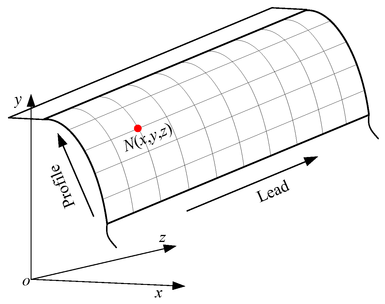
Figure 6.
The loaded transmission error (LTE) and unloaded transmission error (TE) of the helical gear pair with typical manufacturing errors.
Figure 6.
The loaded transmission error (LTE) and unloaded transmission error (TE) of the helical gear pair with typical manufacturing errors.
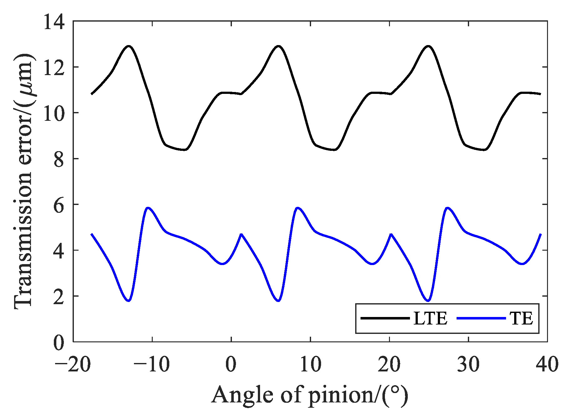
Figure 7.
Comparison of (a) the amplitude of LTE and (b) the load distribution of the tooth surface in two cases: no error and with errors.
Figure 7.
Comparison of (a) the amplitude of LTE and (b) the load distribution of the tooth surface in two cases: no error and with errors.
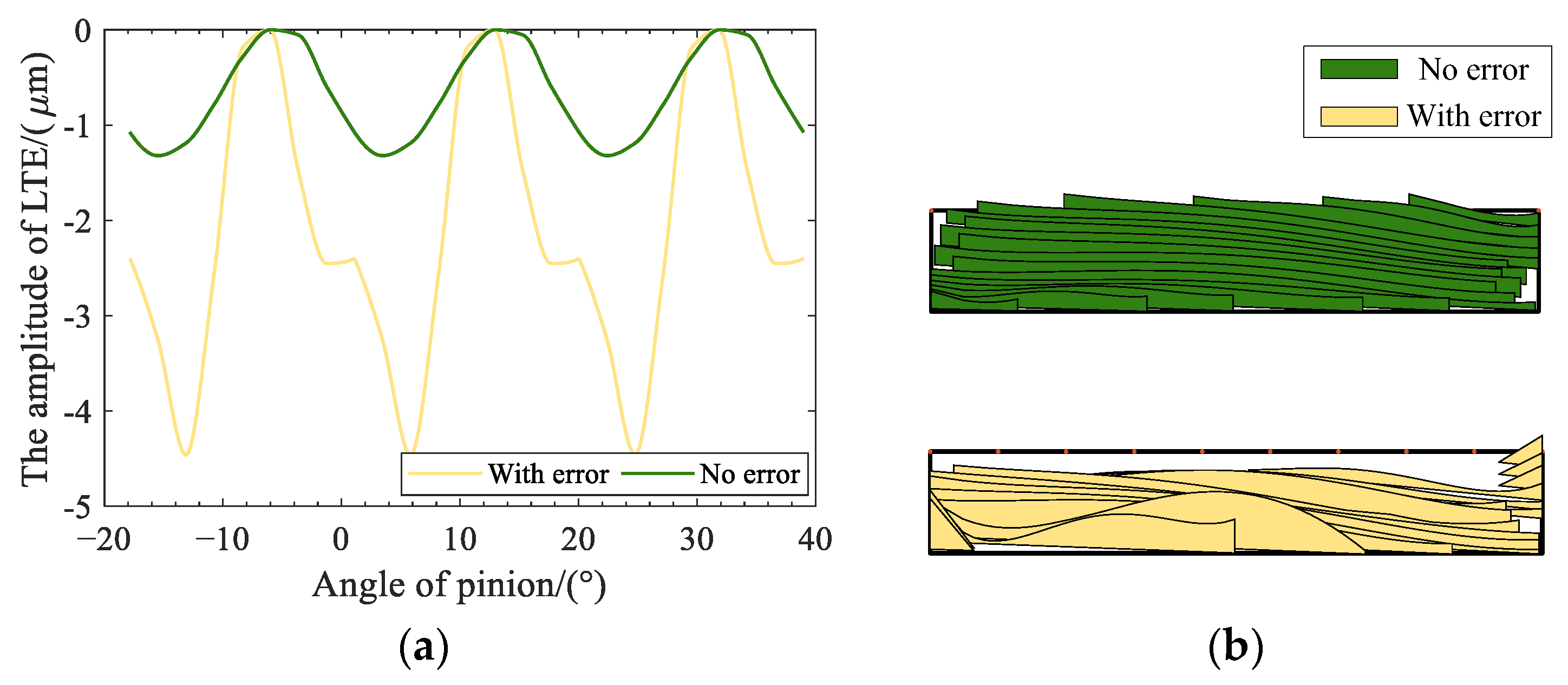
Figure 8.
Time-varying mesh stiffness considering the effect of the manufacturing error.
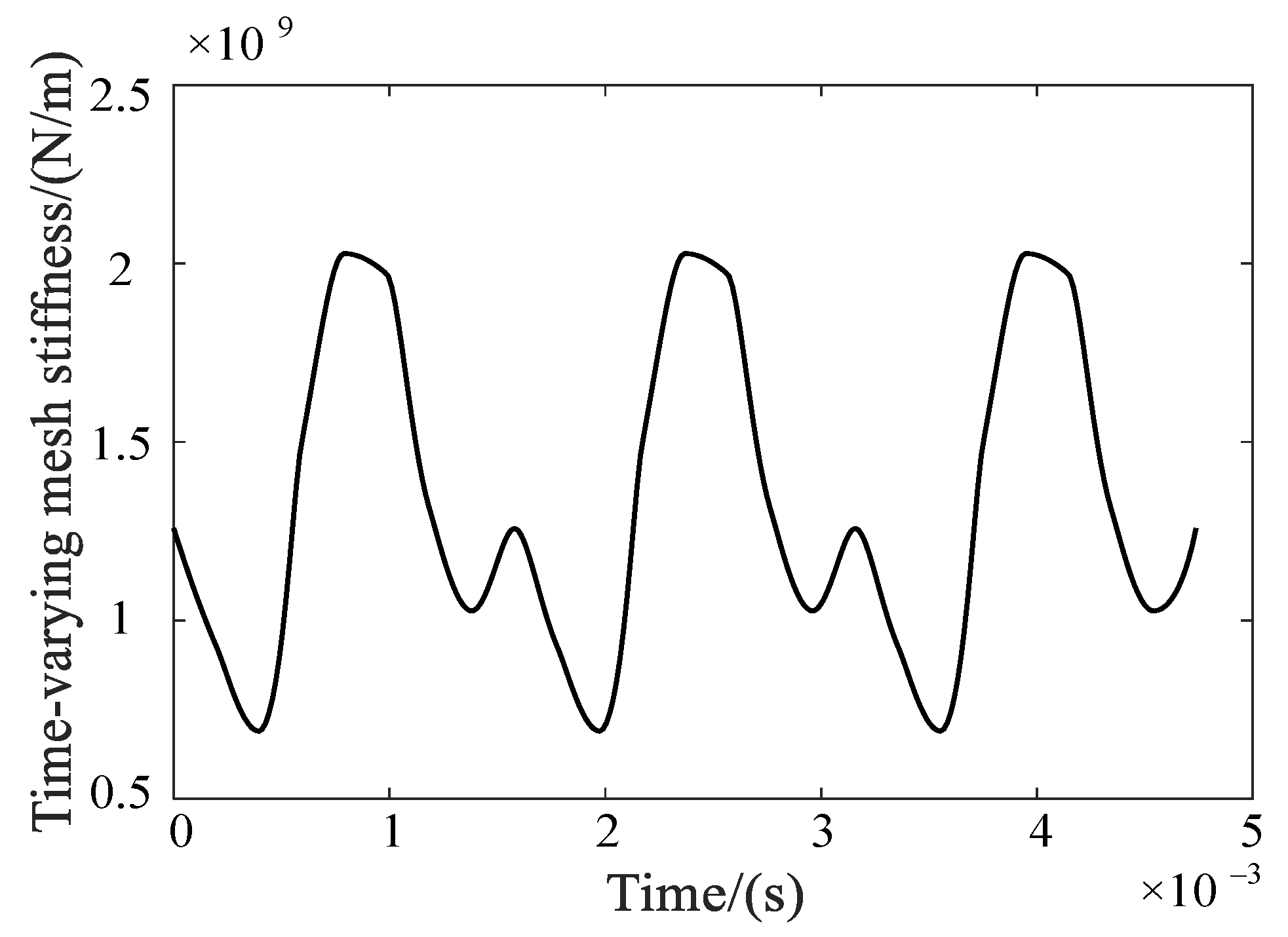
Figure 9.
Sketch map of the actual contact position in the section under the situations of (a) the meshing-in end of the pinion protruding and (b) the meshing-out end of the pinion protruding.
Figure 9.
Sketch map of the actual contact position in the section under the situations of (a) the meshing-in end of the pinion protruding and (b) the meshing-out end of the pinion protruding.
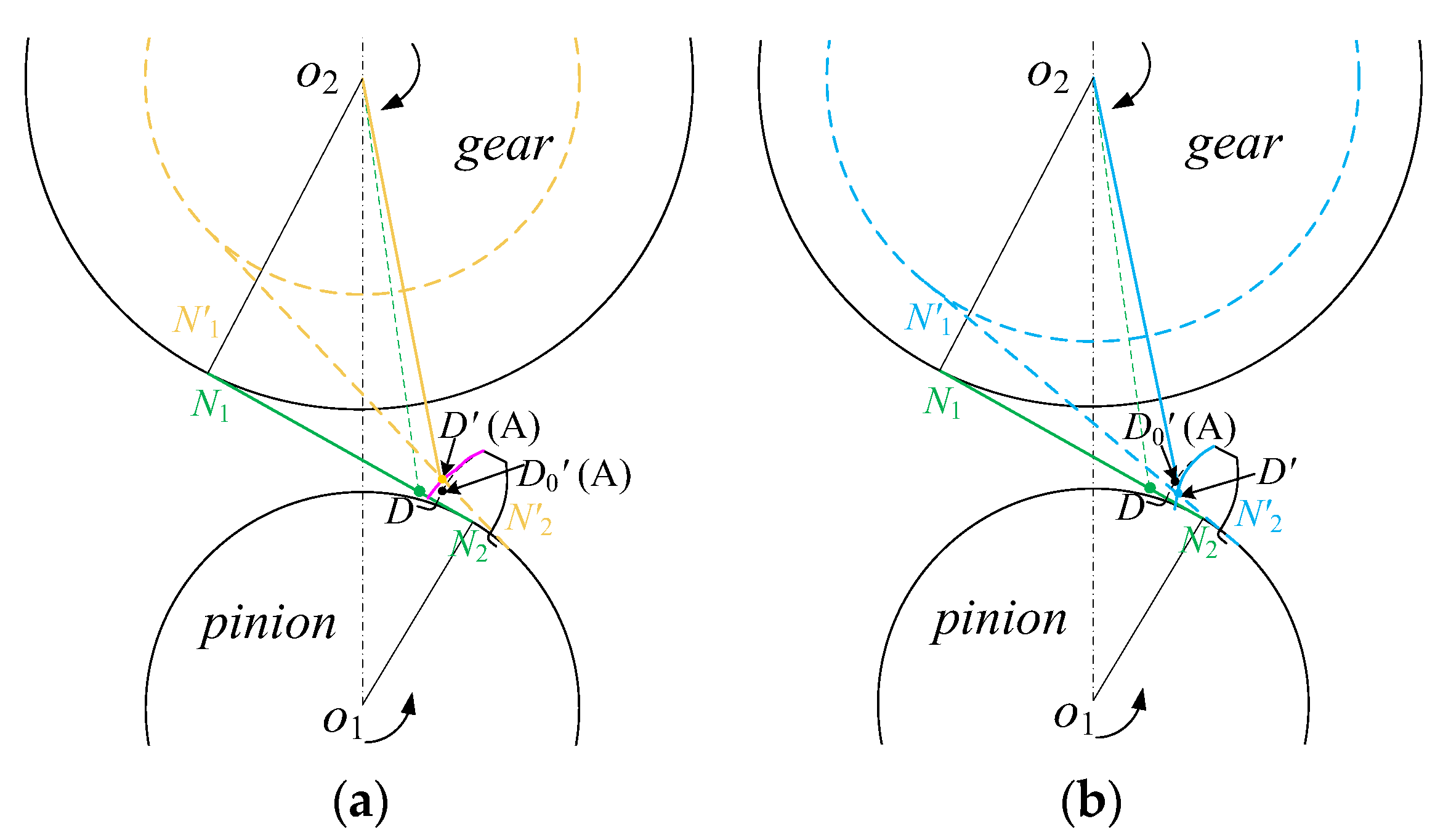
Figure 10.
The geometric relationship of the meshing-in point in the case of the meshing-in end of the pinion protruding.
Figure 10.
The geometric relationship of the meshing-in point in the case of the meshing-in end of the pinion protruding.
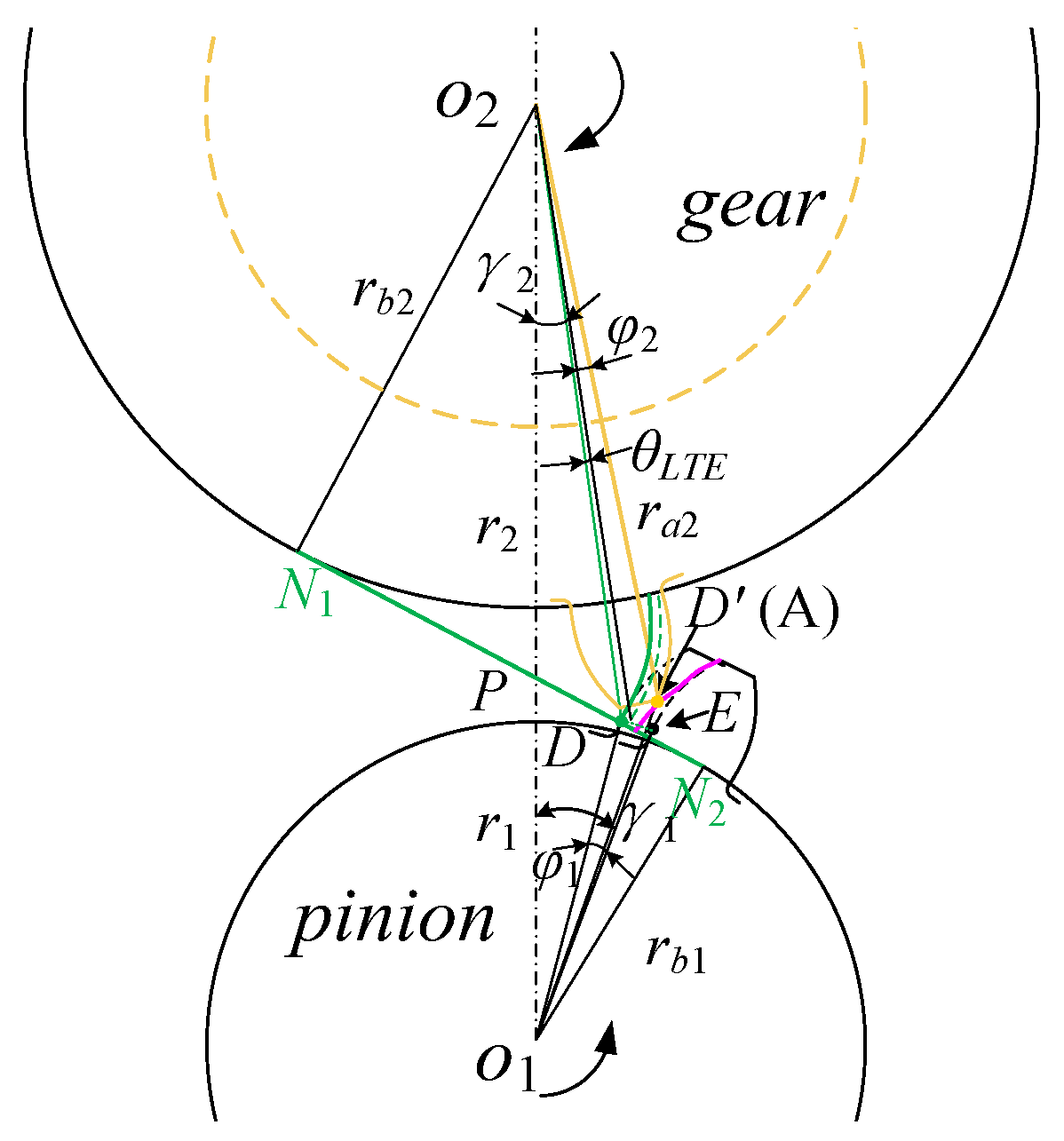
Figure 11.
Approximate location of the original meshing-in point in the case of the meshing-in end of the pinion protruding. (The contact positions on the curve appear in the process from meshing-in to meshing-out for a single tooth).
Figure 11.
Approximate location of the original meshing-in point in the case of the meshing-in end of the pinion protruding. (The contact positions on the curve appear in the process from meshing-in to meshing-out for a single tooth).
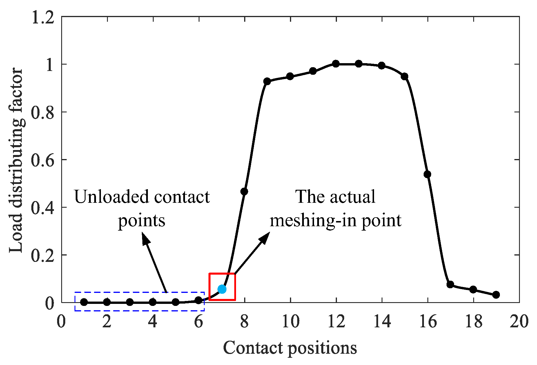
Figure 12.
Meshing-in impact forces for two cases: (a) meshing-in end of the pinion protruding and (b) meshing-out end of the pinion protruding.
Figure 12.
Meshing-in impact forces for two cases: (a) meshing-in end of the pinion protruding and (b) meshing-out end of the pinion protruding.
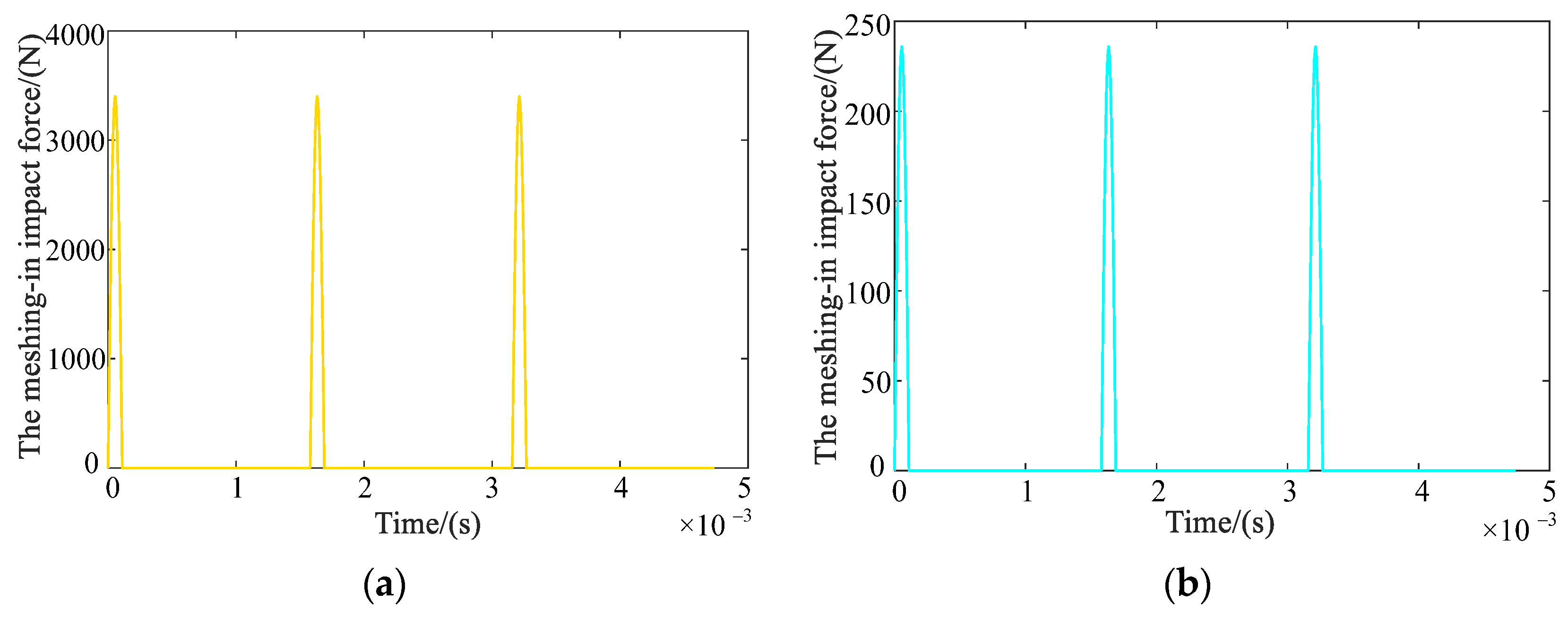
Figure 13.
Dynamic model of the gear transmission system.
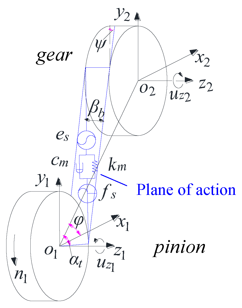
Figure 14.
Framework of the polynomial chaos expansion (PCE) model (a) and the mapping relationship between the error sample and the system response (b).
Figure 14.
Framework of the polynomial chaos expansion (PCE) model (a) and the mapping relationship between the error sample and the system response (b).
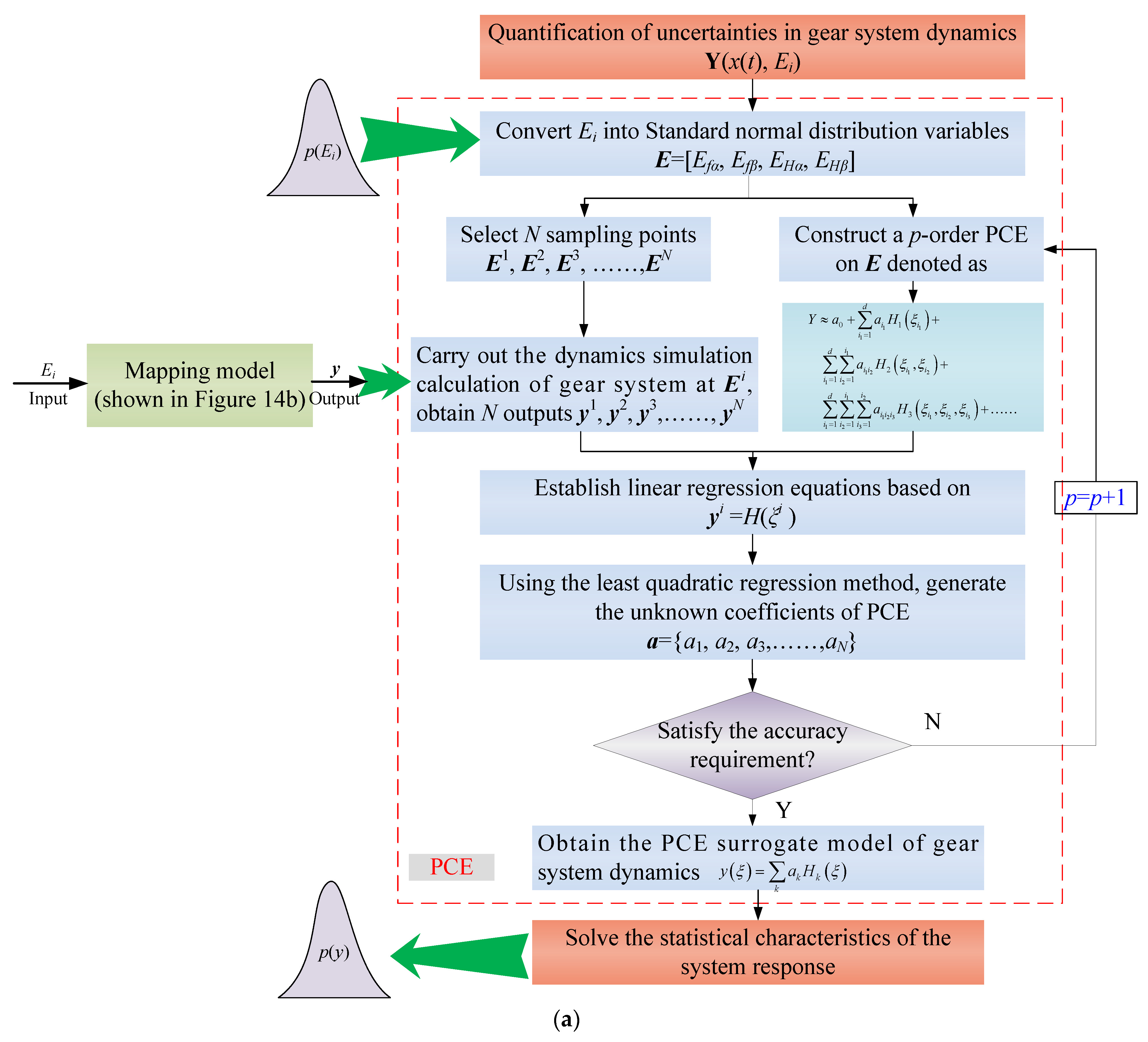
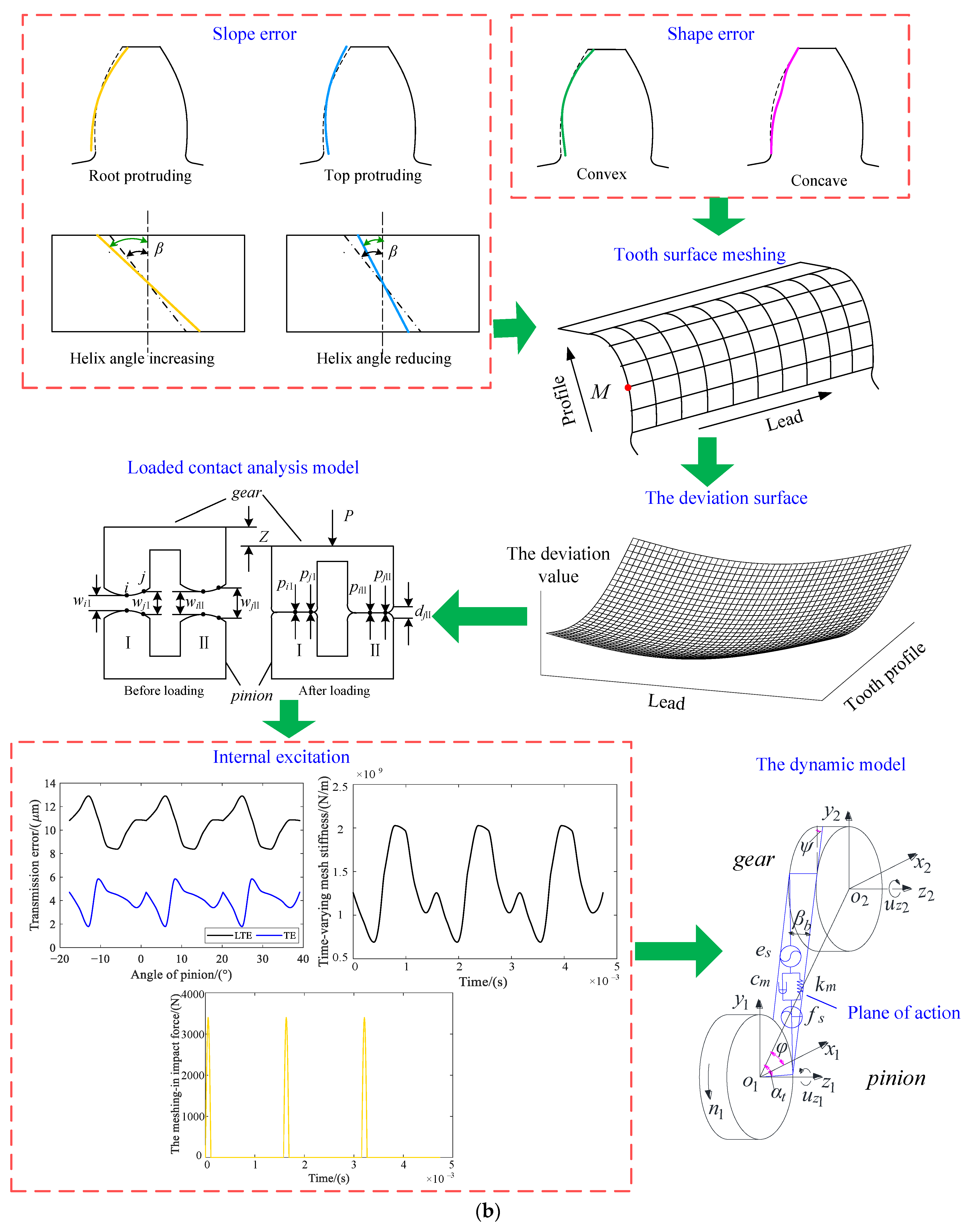
Figure 15.
Dynamic response curve of the gear system under random disturbance with multiple errors, based on the MCS method and PCE models of (a) two-order with N = 30, (b) two-order with N = 60, (c) three-order with N = 70 and (d) three-order with N = 140.
Figure 15.
Dynamic response curve of the gear system under random disturbance with multiple errors, based on the MCS method and PCE models of (a) two-order with N = 30, (b) two-order with N = 60, (c) three-order with N = 70 and (d) three-order with N = 140.
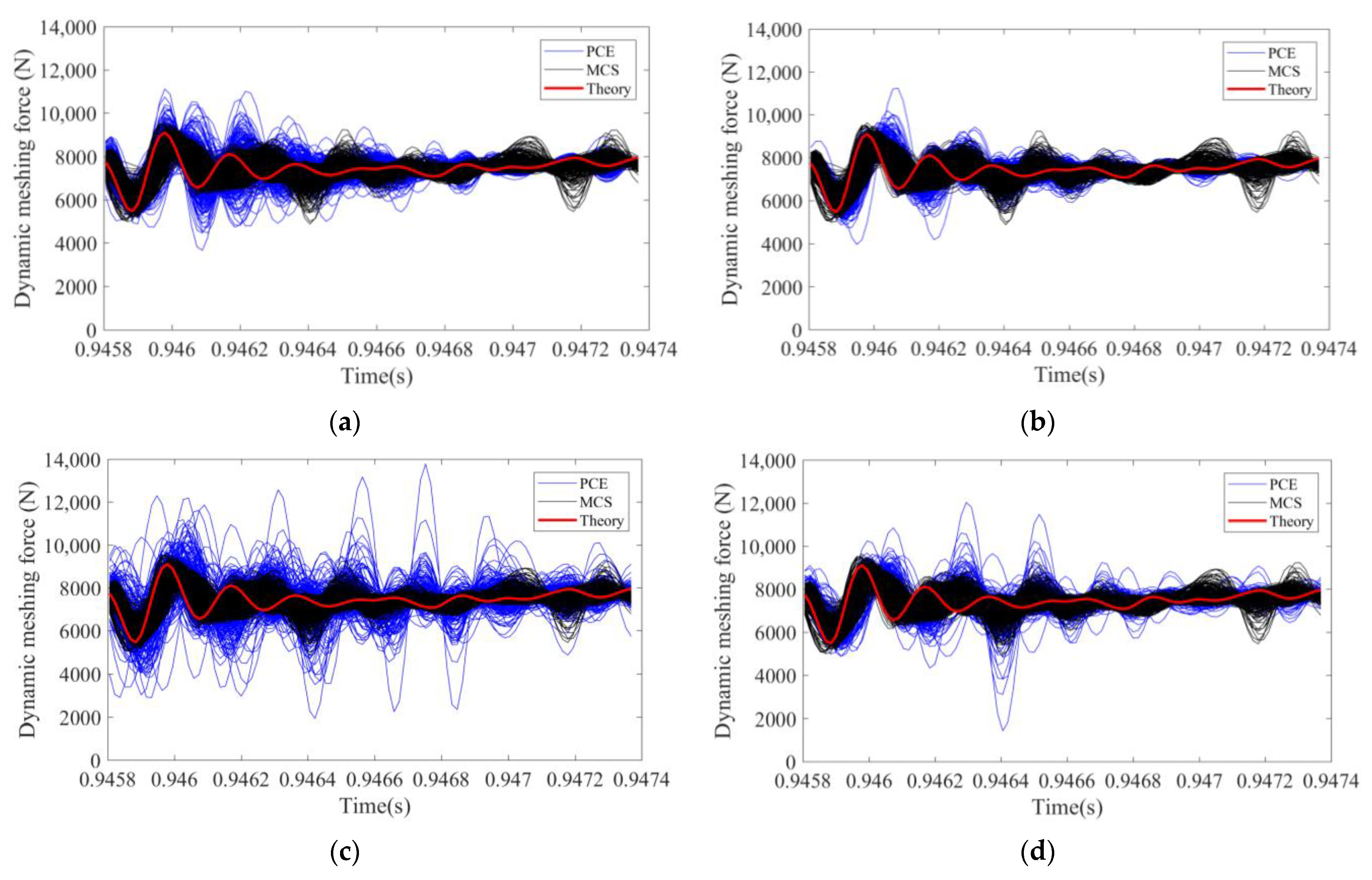
Figure 16.
Relative errors between the MCS method and PCE models of different orders: (a) the mean value and (b) the standard deviation.
Figure 16.
Relative errors between the MCS method and PCE models of different orders: (a) the mean value and (b) the standard deviation.

Figure 17.
Error sensitivity indices under different precisions: (a) grade 5 accuracy, (b) grade 6 accuracy, and (c) grade 7 accuracy.
Figure 17.
Error sensitivity indices under different precisions: (a) grade 5 accuracy, (b) grade 6 accuracy, and (c) grade 7 accuracy.
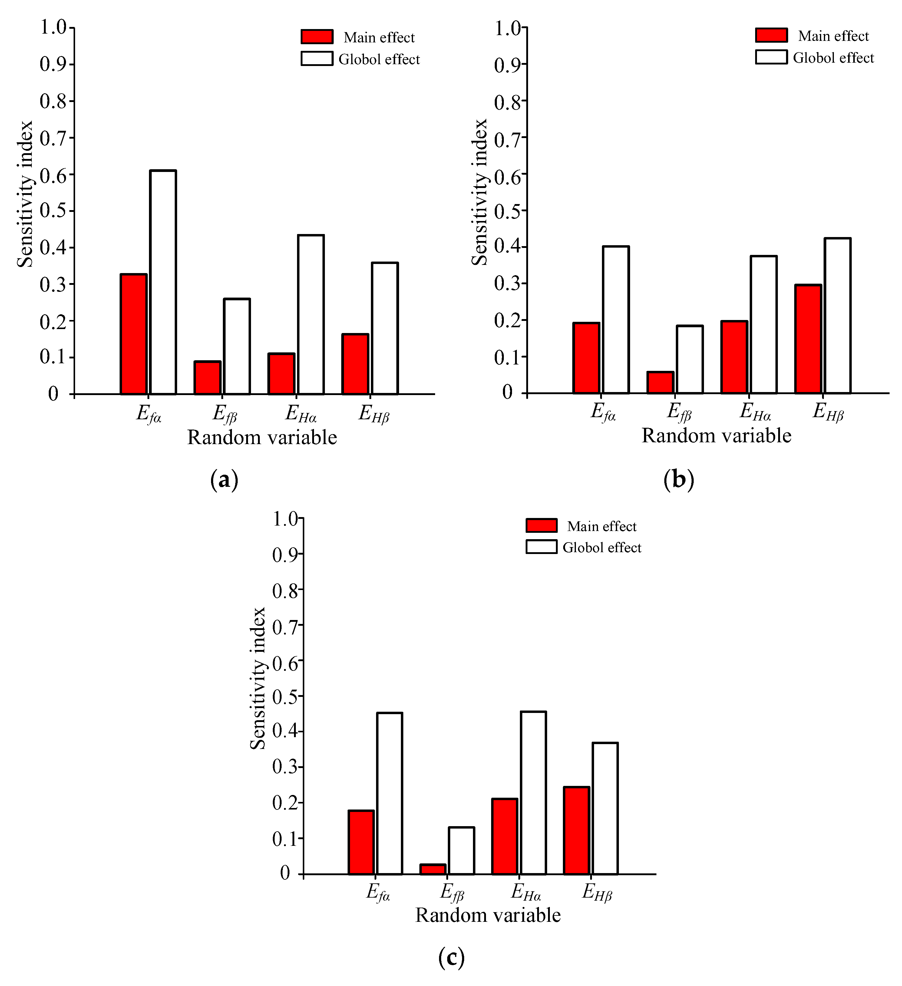
Figure 18.
The total interaction effect between each error and other errors.

Table 1.
The main parameters of the gears.
| Parameters | Pinion | Gear |
|---|---|---|
| Number of teeth, Z1/Z2 | 19 | 47 |
| Handedness | left | right |
| Normal modulus, mn (mm) | 6 | |
| Normal pressure angle, α (°) | 20 | |
| Helix angle, β (°) | 9.91 | |
| Tooth width, B (mm) | 79 | 75 |
| Load torque, T2 (N·m) | 1000 | |
| Input speed, n1 (rpm) | 2000 | |
Table 2.
Value of each error under the specified precision.
| Tooth Profile (μm) | Lead (μm) | ||
|---|---|---|---|
| Shape Error, Efα | Slope Error, EHα | Shape Error, Efβ | Slope Error, EHβ |
| −3 | −3 | −3 | −4 |
(NOTE: The values in parentheses are the tolerance limits for grade 5 precision).
Table 3.
Comparison of system response results based on different methods.
| Method | MCS | PCE | |||
|---|---|---|---|---|---|
| PCE Order and the Sample Size Needed to Determine PCE Coefficient | 2 (M = 15) | 3 (M = 35) | |||
| N = 2M | N = 4M | N = 2M | N = 4M | ||
| Mean value (N) | 3045.86 | 3198.17 | 3045.86 | 3262.95 | 3042.35 |
| Standard deviation (N) | 594.76 | 538.46 | 482.80 | 943.96 | 606.55 |
| Times calling the black-box system model | 1000 | 30 | 60 | 70 | 140 |
| Computing time (h) | 6 | 0.08 | 0.17 | 0.20 | 0.40 |
Table 4.
The comparison of the statistics of the gear meshing performance before and after modification optimization.
Table 4.
The comparison of the statistics of the gear meshing performance before and after modification optimization.
| Accuracy Grade | Tooth Profile | Lead | ||
|---|---|---|---|---|
| Shape Error, Efα | Slope Error, EHα | Shape Error, Efβ | Slope Error, EHβ | |
| 5 | 0.2831 | 0.1714 | 0.3243 | 0.1951 |
| 6 | 0.2095 | 0.1259 | 0.1783 | 0.1274 |
| 7 | 0.2748 | 0.1044 | 0.2457 | 0.1241 |
Disclaimer/Publisher’s Note: The statements, opinions and data contained in all publications are solely those of the individual author(s) and contributor(s) and not of MDPI and/or the editor(s). MDPI and/or the editor(s) disclaim responsibility for any injury to people or property resulting from any ideas, methods, instructions or products referred to in the content. |
© 2023 by the authors. Licensee MDPI, Basel, Switzerland. This article is an open access article distributed under the terms and conditions of the Creative Commons Attribution (CC BY) license (https://creativecommons.org/licenses/by/4.0/).
Share and Cite
MDPI and ACS Style
Guo, F.; Li, C.; Su, J.; Liu, C. Study on Dynamic Uncertainty and Sensitivity of Gear System Considering the Influence of Machining Accuracy. Appl. Sci. 2023, 13, 8011. https://doi.org/10.3390/app13148011
AMA Style
Guo F, Li C, Su J, Liu C. Study on Dynamic Uncertainty and Sensitivity of Gear System Considering the Influence of Machining Accuracy. Applied Sciences. 2023; 13(14):8011. https://doi.org/10.3390/app13148011
Chicago/Turabian StyleGuo, Fang, Chen Li, Jinzhan Su, and Chao Liu. 2023. "Study on Dynamic Uncertainty and Sensitivity of Gear System Considering the Influence of Machining Accuracy" Applied Sciences 13, no. 14: 8011. https://doi.org/10.3390/app13148011
Note that from the first issue of 2016, this journal uses article numbers instead of page numbers. See further details here.