
Band Gap Properties in Metamaterial Beam with Spatially Varying Interval Uncertainties

1
State Key Laboratory of Mechanics and Control for Aerospace Structures, Nanjing University of Aeronautics and Astronautics, Nanjing 210016, China
2
School of Naval Architecture & Ocean Engineering, Jiangsu University of Science and Technology, Zhenjiang 212100, China
*
Author to whom correspondence should be addressed.
Appl. Sci. 2023, 13(14), 8012; https://doi.org/10.3390/app13148012
Submission received: 11 June 2023
/
Revised: 27 June 2023
/
Accepted: 6 July 2023
/
Published: 8 July 2023
(This article belongs to the Special Issue Acoustic Materials and Metamaterials: Advanced Modelling and Characterization Techniques)
Abstract
:First, this study proposed a metamaterial beam model with spatially varying interval density. The interval dynamic equation of this model could be established by incorporating the decomposition results of the interval field based on Karhunen–Loeve expansion into the finite element method. An interval perturbation finite element method was developed to evaluate the bounds of the dynamic response interval vector. Then, an interval vibration transmission analysis could be performed, and the frequency range of the safe band gap could be determined. Meanwhile, Monte Carlo simulations and the vertex method are also presented to provide reference solutions. By comparison, it was found that the calculation accuracy of the interval perturbation finite element method was acceptable. The numerical results also showed that the safe band gap range was significantly smaller than that of the deterministic band gap.
1. Introduction
Acoustic metamaterials are artificial periodic materials with unique band gap properties [1,2]. The band gap represents the range of frequencies in which elastic waves are always attenuated when propagating through acoustic metamaterials. Therefore, acoustic metamaterials can provide a new research direction for vibration control. Metamaterials are formed by the periodic arrangement of several specially designed microstructures, and it is the locally resonant mechanism of such microstructures that leads to the generation of band gaps [3]. Hence, the band gap is usually near the natural resonance frequency of the microstructure.
So far, researchers have constructed diverse metamaterial beam (MB) structures by periodically adding various forms of microstructures to basic beams. Xiao et al. [4] formed a basic model of a metamaterial beam by periodically attaching a series of resonators to a homogeneous beam. It was found that both the resonant and the Bragg scattering band gaps existed in the model. Wang et al. [5] attached multioscillators periodically to a basic beam to obtain multiple band gaps. Some researchers have proposed reducing the band gap frequency range of metamaterial beams by introducing a negative stiffness mechanism into the resonators [6,7,8]. Guo et al. [9] studied the wave characteristics of a double-layer metamaterial beam structure using the transfer matrix method and found that its vibration reduction effect was better than that of the traditional metamaterial beam. In addition, there are other resonators of different forms, such as beam-like resonators [10], continuum-beam resonators [11], and 2-DOF type resonators [12], which can all contribute to the formation of unique band gaps.
The above-mentioned methods for calculating band gaps were all based on the spatial periodicity of metamaterial structures. However, due to some uncontrollable factors, the design parameters are often affected by spatial uncertainties. Such spatial uncertainties are often difficult to measure and break the assumption of spatial periodicity to some extent. When statistical data are seriously lacking, one can simply consider that the value of the uncertain parameter only fluctuates within a certain known interval range, and the corresponding interval model becomes the most appropriate method for analyzing uncertainties. In the interval model, the interval field methods that can be applied to deal with spatial uncertainties fall into three main categories: (1) the explicit interval field formulation, (2) interval fields based on Karhunen–Loeve (KL) expansion, and (3) interval fields based on convex models. Following explicit formulation, an interval field can be interpreted as the superposition of base functions scaled by interval coefficients [13]. The interval coefficients are uncertain, but the base functions are deterministic, which ensures the spatial continuity of the uncertain parameters. The specific form of the base functions often depends on the engineering experience and intuitive judgment of the researchers. Sofi et al. [14,15,16,17] proposed using KL decomposition to obtain the base functions. KL expansion quantifies the spatial dependency of the interval field by defining the spatial dependency function. Recently, some scholars have used convex models to describe interval field problems. Similarly, the convex model uses the auto-dependence function to describe the spatial dependence of the interval field [18,19,20,21]. The commonly used convex models include the ellipsoidal model [22], multidimensional parallelepiped model [23], and improved multidimensional parallelepiped model [24].
Wu et al. [25] and He et al. [26] used the interval analysis technique and stochastic analysis technique, respectively, to study the uncertainties in acoustic metamaterials. However, there have been no studies on spatial uncertainties in acoustic metamaterials. Therefore, after introducing the band gap calculation method for deterministic metamaterial beams in detail, a metamaterial beam model with spatially varying interval density is first proposed in this paper. Section 2 introduces the main features of this model, and an interval perturbation finite element method (IPFEM) is proposed to study the dynamic response of this model. In Section 3, numerical examples are presented to demonstrate the efficiency and accuracy of the IPFEM. Finally, the conclusions are summarized in Section 4.
2. The Model and Method
After briefly introducing the band gap calculation method for a deterministic MB in Section 2.1, an interval MB structure with spatial uncertainties is established in this section. The flowchart for solving the dynamic response of this interval MB structure is shown in Figure 1. Firstly, assuming the density of the basic beam contains spatial uncertainties, the interval field based on KL expansion is used to deal with these uncertainties in Section 2.2. Then, in Section 2.3, the interval field decomposition results are introduced into the finite element method to obtain the interval dynamic equation. Next, an interval perturbation finite element method is proposed to solve this interval dynamic equation in Section 2.4. Finally, an interval vibration transmission analysis is implemented in Section 2.5 to intuitively reflect the influence of spatial uncertainties on the band gap.
2.1. Deterministic Metamaterial Beam Structure and Its Band Gap Calculation
Before analyzing the spatial uncertainties in the metamaterial beam, this subsection briefly introduces the deterministic metamaterial beam structure and its band gap calculation method. As shown in Figure 2, a finite conventional MB structure with unit cells is formed by periodically attaching a series of resonators to a uniform aluminum beam. The lattice constant is a, and the width and thickness of the aluminum beam are denoted as b and h, respectively. Each resonator contains a spring k and a mass m. Each unit cell contains Euler–Bernoulli beam elements. Thus, the uniform aluminum beam can be divided into beam elements. It is worth emphasizing that must be even so that the spring mass resonator can be located just on the node. The stiffness matrix and mass matrix of the Euler–Bernoulli beam element are shown in Ref. [8]. After assembling these elements, the global stiffness matrix and global mass matrix of the aluminum beam can be obtained. It should be noted that node numbering is carried out from left to right along MB during assembly. Furthermore, the global dynamic stiffness matrix of the aluminum beam can be obtained as follows:
Here, is the circular frequency. On the other hand, the influence of the spring mass resonator on the dynamic behavior of the MB can be obtained by the methodology described in Ref. [4]. The dynamic effect matrix of the spring mass resonator is defined as follows:
Has the same dimensions as . Obviously, the global dynamic stiffness matrix of the metamaterial beam is equal to . The dynamic equation of the finite MB can be written in the following form:
where is the dynamic response vector and is the structural load vector.
The band gap frequency range can usually be determined by performing a vibration transmission analysis. The transmission coefficient of vibration T is defined as:
In the above, and represent the displacements of the excitation point and the response point, respectively. The left and right ends of the metamaterial beam are selected as the excitation and response points, respectively. Therefore, and are located in the first and penultimate rows of the vector , respectively. Assuming that the displacement of the excitation point is 1 (), the implementation method is: (1) modify to a value far greater than the other elements in , such as ; (2) define as follows:
Finally, solving Equation (3) yields . If is greater than , namely, T is less than 0, it indicates that the flexural wave is attenuated when propagating through the metamaterial beam. Therefore, the frequency range wherein T is less than zero is the band gap.
2.2. Uncertain Density Modeled as an Interval Field
In the deterministic metamaterial beam structure, the basic beam (aluminum beam) is considered to be homogeneous. Obviously, the basic beam may have spatially varying uncertainties under the influence of many uncertain factors. In order to study the effect of spatial uncertainties on the band gap, an interval field model based on KL expansion is used to deal with the spatially varying uncertainties. In the interval field model, the correlation between physical parameters at different positions is defined by the spatial dependency function. Then, the spatial dependency function is expanded into the form of the superposition of base functions by KL decomposition, which guarantees the spatial continuity of the physical parameters and reduces the number of interval parameters. It is assumed that the density of the basic beam has spatially varying uncertainties, and its form is:
Here, the superscript I represents the interval quantities; and denote the lower and upper bounds of the interval field, respectively; and represents the length of the basic beam. The midpoint and deviation amplitude of the interval field can be expressed by Equation (7).
The interval field can also be written in dimensionless form:
Here, represents a dimensionless interval function whose midpoint is zero. The spatial dependency function of at different positions and can be defined as:
Here, indicates the midpoint symbol. can be expanded using KL expansion technology:
where represents the nth eigenvalue of and is the corresponding eigenfunction. According to Equations (9) and (10), and retaining the first N terms in KL expansion, we can obtain:
where is an interval parameter , whose deviation amplitude is equal to 1. Substituting Equation (11) into Equation (8) gives
In this paper, we assume that has the following exponential form:
Here, and are parameters affecting the deviation amplitude and the spatial dependency of the interval field, respectively.
2.3. Interval Field Finite Element Formulation
In this subsection, the results of the interval field decomposition shown in Equation (12) are introduced into the finite element method, and the deterministic dynamic equation shown in Equation (3) is extended to the interval dynamic equation. As shown in Figure 3, a coordinate system is established along the direction of the basic beam. The origin is established at the left end of the metamaterial beam, while represents the coordinate of the left end of the nth beam element. As we all know, density only affects the system mass matrix, and the interval mass matrix of the nth beam element can be obtained by integration as follows:
Here, stands for the shape function matrix, and is the area of the cross-section. Substituting Equation (12) into Equation (14), can be recast as:
Here, and . After assembly, the interval global mass matrix of the basic beam can be expressed in the following form:
where
Here, is the connectivity matrix of the nth element. Furtherly, the interval dynamic equation of the metamaterial beam can be expressed as:
where
Here, represents the interval global dynamic stiffness matrix, and is the dynamic response interval vector. Similarly, in order to make always equal to 1, needs to be changed to , and needs to be changed to 0. still represents the structural load vector, which is defined according to Equation (5). Hence, is not an interval vector.
2.4. Interval Perturbation Finite Element Method (IPFEM)
A classical method to solve Equation (18) is IPFEM. The core of IPFEM is to use the first-order Taylor series to expand the dynamic stiffness matrix and then use the first-order Neumann series to approximate the inverse of the interval dynamic stiffness matrix and finally obtain the derivative of the dynamic response interval vector with respect to . The first-order Taylor series expansion of around can be expressed as:
where is the midpoint of , which is the solution to Equation (18) when . denote the deviation amplitude of . can be obtained as:
Therefore, can be expressed as:
Finally, the lower and upper bounds of can be calculated by:
2.5. Interval Vibration Transmission Analysis (IVTA)
Finally, this paper proposes studying the effect of spatial uncertainties on the band gap by implementing interval vibration transmission analysis. The penultimate rows of and represent the lower bound and upper bound of , respectively. Then, we can define the interval transmission coeffcient as follows:
where
Here, and denote the lower and upper bounds of the interval transmission coeffcient, respectively. By observing Equation (26), it can be found that when , , which makes the specific value of the coeffcient difficult to obtain. Therefore, only the coeffcient is presented in the numerical examples of this paper.
3. Results and Discussion
This section mainly includes the following parts. First, the band gap calculation of a deterministic MB is presented. Then, a numerical example is investigated to validate the accuracy of the IPFEM in analyzing a metamaterial beam with spatial uncertainties regarding density. Meanwhile, the Monte Carlo method (MCM) with a million samples and the vertex method (VM) are also implemented as reference methods. Next, the effects of the number of terms in KL expansion and the interval field parameters on the band gap behavior are investigated. Finally, on the basis of the above interval field analysis, the effect of resonator uncertainties is further studied.
3.1. Band Gap Analysis of Deterministic Metamaterial Beam
Figure 4 displays the transmission coefficient curve of a deterministic MB. This deterministic MB contains a total of 12 unit cells, and each unit cell consists of four beam elements. The lattice constant a is 0.07 m. The thickness h and width b of the basic beam are equal to 0.0025 m and 0.01 m, respectively. The mass m and spring stiffness k are equal to 0.0225 kg and 769.04 N/m, respectively. The Young’s modulus E and density of aluminum are equal to Pa and , respectively. As shown in the shaded areas in Figure 4, this metamaterial beam can form a band gap from 29.4452 Hz to 69.9634 Hz.
3.2. Metamaterial Beam with Interval Density Field
In this subsection, the density of a basic beam is considered to contain spatial uncertainties. The midpoint of the interval density field is . The number of terms in KL expansion is N = 10. The interval field parameters and are equal to 0.05 and , respectively. The other parameters are the same as in Section 3.1. Thus, an IVTA can be carried out, and its results are displayed in Figure 5. For comparison, Figure 5 also shows the deterministic IVTA results (midpoint line), i.e., the calculation results in Figure 4. The yellow line, blue line, and red line represent the coefficient calculated by IPFEM, VM, and MCM, respectively. The four curves in Figure 5 basically coincide at the low frequency range. However, when the frequency gradually approaches the ending frequency of the band gap, the coefficient deviates obviously from the deterministic analysis results. For convenience, the frequency range where the upper bound of the interval transmission coeffcient is less than 0 is referred to as the safe band gap. No matter how the interval density field fluctuates, the metamaterial beam structure can always provide vibration attenuation in the frequency range of the safe band gap. For example, the safe band gap obtained by the two reference methods (MCM and VM) ranged from 29.4452 Hz to 67.7894 Hz (see the purple rectangular frame in Figure 5), which reduced the frequency range of the safe band gap by compared to the deterministic band gap range. However, in fact, near the ending frequency, the curves representing the calculation results of the VM and MCM did not coincide exactly. For the IPFEM, the safe band gap ranged from 29.4452 Hz to 69.3760 Hz (see the light blue frame in Figure 5). In order to validate the calculation precision of the IPFEM, the relative error of the IPFEM with respect to the MCM was also calculated as follows:
where represents the beginning frequency or ending frequency of the safe band gap calculated by the IPFEM, and denotes the beginning frequency or ending frequency of the safe band gap calculated by the MCM. That is to say, in the numerical example shown in Figure 5, the relative error of the beginning frequency of the safe band gap is , and the relative error of the ending frequency is . At the same time, the calculated result curve of the IPFEM in Figure 5 also had a certain deviation from the two reference methods near the ending frequency. The reason for this was that there was a natural frequency near the ending frequency, and the nonlinearity was strengthened near the natural frequency, which led to the gradual deviation of the calculation results of various interval methods [27,28]. In other words, due to the spatial uncertainties of the density of the basic beam, the safe band gap frequency range was narrower than the deterministic band gap frequency range (29.4452–69.9634 Hz). Specifically, only the ending frequency of the safe band gap is affected by the spatial uncertainties of the density of a basic beam, but the beginning frequency is not. This is mainly because, in the deterministic metamaterial beam structure, the beginning frequency is and the ending frequency is [6]. Obviously, the uncertainties of the density of a basic beam only affect the ending frequency.
3.3. Influences of the Number of Terms in KL Expansion on the Safe Band Gap
Figure 6 displays the convergence of the ending frequency of the safe band gap with the number of terms N in KL expansion under three different cases. N takes the first 15 orders in MCM and IPFEM. However, in the vertex method, the computation time increases dramatically as N increases. When N is greater than 11, the computational efficiency is extremely low. Thus, only the first 11 orders of N are taken in the vertex method. It can be seen that a larger N denotes a more accurate interval density field simulation; thus, the ending frequency of the safe band gap is also more accurate. But it also means more computing time. In these three figures, the ending frequencies obtained by the three methods all changed rapidly when and became stable until N was near 10. Considering the calculation accuracy and efficiency comprehensively, the final value of N was determined to be 10. Another interesting phenomenon is that in all the numerical examples presented in these three figures, as N increased, the ending frequencies obtained by the MCM and VM gradually coincided. However, the ending frequency obtained by the IPFEM was always higher than the calculation results of the MCM and VM.
3.4. Influences of Interval Field Parameters on the Safe Band Gap
In this subsection, we further study the influences of interval field parameters and on the safe band gap, and the results are presented in Figure 7. It was observed that the calculation results of the MCM and VM were in perfect agreement. In Figure 7a, as increased, the ending frequency of the safe band gap gradually decreased, which led to the gradual narrowing of the safe band gap. Obviously, the greater the deviation amplitude of the interval field, the greater the influences of spatial uncertainties on the band gap. In Figure 7b, as increased, the ending frequencies obtained by the MCM and VM increased significantly, while the ending frequency obtained by the IPFEM increased slightly. In other words, the stronger the spatial dependency of the interval field, the weaker the influences of spatial uncertainties on the band gap. In addition, as shown in Figure 7, the ending frequency obtained by the IPFEM was always higher than the reference solutions (MCM and VM). To validate the accuracy of the IPFEM, Figure 8 shows the relative errors of the IPFEM with respect to the MCM. As can be seen from Figure 8, an increase in or a decrease in led to an increase in relative errors. However, the relative errors presented in Figure 8 were basically controlled within .
3.5. Metamaterial Beam with Interval Density Field and Interval Resonator
Since there may be uncertainties in the basic beam, it is obvious that there may be uncertainties in the spring-mass resonator. The spring stiffness and mass in each resonator can be assumed to be an independent interval variable and expressed as follows:
The values of m and k are shown in Section 3.1. and denote the dimensionless deviation amplitude of and , respectively. Figure 9a shows the IVTA results considering both the uncertainties in the density of the basic beam () and the uncertainties in the resonators (). It should be noted that due to the extremely low computational efficiency, the vertex method was not used in the numerical examples presented in this subsection. When the interval parameters of the resonators were added into the calculation, the beginning frequency was also influenced by uncertainties. The safe band gap range predicted by the MCM was from 29.7639 Hz to 67.2779 Hz, reducing the band gap width by compared to the deterministic band gap. Furthermore, the safe band gap range obtained by the IPFEM was from 29.9966 Hz to 69.3091 Hz. Both the beginning frequency and the ending frequency were higher than those obtained by the MCM, and the relative errors were and , respectively. Another IVTA could be implemented by keeping interval field parameters and unchanged and increasing and to 0.04. The calculation results are presented in Figure 9b. In Figure 9b, the safe band gap calculated by the MCM ranged from 29.8576 Hz to 66.7813 Hz, reducing the band gap width by . Meanwhile, the safe band gap calculated by the IPFEM was from 30.0621 Hz to 69.1674 Hz. Similarly, the beginning frequency and ending frequency were higher than those obtained by the MCM, and the relative errors were and , respectively. That is to say, the IPFEM could not provide a conservative solution for the safe band gap, but its calculation precision was acceptable.
4. Conclusions
In this paper, a metamaterial beam model with spatially varying interval density was first established. Then, the interval dynamic equation could be obtained by integrating the decomposition result of the interval field based on KL expansion into the standard finite element formulation. Next, an IPFEM was applied to obtain the bounds of the dynamic response interval vector. Finally, an IVTA was carried out to intuitively reflect the uncertainties in the transmission coefficient of vibration. Meanwhile, the MCM and VM were also presented as reference methods.
For convenience, the frequency range wherein the upper bound of the interval transmission coeffcient is less than 0 is called the safe band gap. No matter how the interval density field fluctuates, the elastic wave within the safe band gap cannot propagate through the metamaterial beam. In other words, in engineering, if researchers only know the specific ranges of uncertainties in the MB structures but cannot determine the exact values, they can use the method in this paper to deal with the uncertainties and calculate the safe band gap. Then, using the safe band gap range instead of the deterministic band gap range can ensure that the metamaterial beam always provides vibration attenuation characteristics and is safe enough during application processes.
The numerical results showed that the interval density field of the basic beam could only affect the ending frequency of the safe band gap. On the other hand, the uncertainties of the resonators affected both the beginning frequency and ending frequency of the safe band gap. When both the uncertainties in the density of the basic beam and the uncertainties in the resonators were considered, the safe band gap range could be reduced by compared to the deterministic band gap without considering uncertainties. In the numerical examples presented in this paper, the beginning frequency calculated by the IPFEM was basically the same as the reference solutions, but the ending frequency was always higher than the reference solutions. In other words, the IPFEM could not obtain a conservative safe band gap frequency range. However, the relative errors of the IPFEM were basically less than , and its calculation precision could basically meet the engineering requirements. This paper only considered a one-dimensional metamaterial beam structure. Next, the authors of this paper will try to study the uncertainties in two-dimensional or three-dimensional metamaterial structures based on the secondary development platform of finite element software.
Author Contributions
Conceptualization, F.H. and Z.S.; methodology, F.H. and X.F.; software, F.H., Z.Z. and X.F.; validation, F.H.; formal analysis, F.H.; investigation, F.H.; resources, Z.S. and D.Q.; data curation, F.H.; writing—original draft preparation, F.H.; writing—review and editing, Z.S.; visualization, F.H.; supervision, Z.S.; project administration, Z.S. and D.Q. All authors have read and agreed to the published version of the manuscript.
Funding
This work was funded by the National Natural Science Foundation of China (grant No. 12272172), the Natural Science Foundation of Jiangsu Higher Education Institutions of China (No. 22KJB580005), the Youth Talent Promotion Project from China Association for Science and Technology (2022QNRC001), and the Priority Academic Program Development of Jiangsu Higher Education Institutions.
Institutional Review Board Statement
Not applicable.
Informed Consent Statement
Not applicable.
Data Availability Statement
Not applicable.
Conflicts of Interest
The authors declare no conflict of interest.
References
- Meng, H.; Chronopoulos, D.; Fabro, A.; Maskery, I.; Chen, Y. Optimal design of rainbow elastic metamaterials. Int. J. Mech. Sci. 2020, 165, 105185. [Google Scholar] [CrossRef]
- Wei, W.; Ren, S.; Chronopoulos, D.; Meng, H. Optimization of connection architectures and mass distributions for metamaterials with multiple resonators. J. Appl. Phys. 2021, 129, 165101. [Google Scholar] [CrossRef]
- Liu, Z.; Zhang, X.; Mao, Y.; Zhu, Y.Y.; Yang, Z.; Chan, C.T.; Sheng, P. Locally Resonant Sonic Materials. Science 2000, 289, 1734–1736. [Google Scholar] [CrossRef] [PubMed]
- Xiao, Y.; Wen, J.; Yu, D.; Wen, X. Flexural wave propagation in beams with periodically attached vibration absorbers: Band-gap behavior and band formation mechanisms. J. Sound Vib. 2013, 332, 867–893. [Google Scholar] [CrossRef]
- Wang, Z.; Zhang, P.; Zhang, Y. Locally Resonant Band Gaps in Flexural Vibrations of a Timoshenko Beam with Periodically Attached Multioscillators. Math. Probl. Eng. 2013, 2013, 1–10. [Google Scholar] [CrossRef] [Green Version]
- Zhou, J.; Wang, K.; Xu, D.; Ouyang, H. Local resonator with high-static-low-dynamic stiffness for lowering band gaps of flexural wave in beams. J. Appl. Phys. 2017, 121, 044902. [Google Scholar] [CrossRef] [Green Version]
- Wu, Q.; Huang, G.; Liu, C.; Xie, S.; Xu, M. Low-frequency multi-mode vibration suppression of a metastructure beam with two-stage high-static-low-dynamic stiffness oscillators. Acta Mech. 2019, 230, 4341–4356. [Google Scholar] [CrossRef]
- He, F.Y.; Shi, Z.Y.; Qian, D.H.; Tu, J.; Chen, M.L. Flexural wave bandgap properties in metamaterial dual-beam structure. Phys. Lett. 2022, 429, 127950. [Google Scholar] [CrossRef]
- Guo, Z.; Hu, G.; Sorokin, V.; Tang, L.; Yang, X.; Zhang, J. Low-frequency flexural wave attenuation in metamaterial sandwich beam with hourglass lattice truss core. Wave Motion 2021, 104, 102750. [Google Scholar] [CrossRef]
- Xiao, Y.; Wen, J.; Wang, G.; Wen, X. Theoretical and Experimental Study of Locally Resonant and Bragg Band Gaps in Flexural Beams Carrying Periodic Arrays of Beam-Like Resonators. J. Vib. Acoust. 2013, 135, 041006. [Google Scholar] [CrossRef]
- Wang, X.; Wang, M.Y. An analysis of flexural wave band gaps of locally resonant beams with continuum beam resonators. Meccanica 2016, 51, 171–178. [Google Scholar] [CrossRef]
- Lv, H.; Zhang, Y. A Wave-Based Vibration Analysis of a Finite Timoshenko Locally Resonant Beam Suspended with Periodic Uncoupled Force-Moment Type Resonators. Crystals 2020, 10, 1132. [Google Scholar] [CrossRef]
- Verhaeghe, W.; Desmet, W.; Vandepitte, D.; Moens, D. Interval fields to represent uncertainty on the output side of a static FE analysis. Comput. Methods Appl. Mech. Eng. 2013, 260, 50–62. [Google Scholar] [CrossRef]
- Sofi, A.; Muscolino, G. Static analysis of Euler-Bernoulli beams with interval Young’s modulus. Comput. Struct. 2015, 156, 72–82. [Google Scholar] [CrossRef]
- Sofi, A. Structural response variability under spatially dependent uncertainty Stochastic versus interval model. Probabilistic Eng. Mech. 2015, 42, 78–86. [Google Scholar] [CrossRef]
- Sofi, A. Euler-Bernoulli interval finite element with spatially varying uncertain properties. Acta Mech. 2017, 228, 3771–3787. [Google Scholar] [CrossRef]
- Sofi, A.; Romeo, E.; Barrera, O.; Cocks, A. An interval finite element method for the analysis of structures with spatially varying uncertainties. Adv. Eng. Softw. 2019, 128, 1–19. [Google Scholar] [CrossRef]
- Ni, B.Y.; Wu, P.G.; Li, J.Y.; Jiang, C. A semi-analytical interval method for response bounds analysis of structures with spatially uncertain loads. Finite Elem. Anal. Des. 2020, 182, 103483. [Google Scholar] [CrossRef]
- Jiang, C.; Han, X.; Lu, G.Y.; Liu, J.; Zhang, Z.; Bai, Y.C. Correlation analysis of non-probabilistic convex model and corresponding structural reliability technique. Comput. Methods Appl. Mech. Eng. 2011, 200, 2528–2546. [Google Scholar] [CrossRef]
- Jiang, C.; Bi, R.G.; Lu, G.Y.; Han, X. Structural reliability analysis using non-probabilistic convex model. Comput. Methods Appl. Mech. Eng. 2013, 254, 83–98. [Google Scholar] [CrossRef]
- Li, J.W.; Ni, B.Y.; Jiang, C.; Fang, T. Dynamic response bound analysis for elastic beams under uncertain excitations. J. Sound Vib. 2018, 422, 471–489. [Google Scholar] [CrossRef]
- Ni, B.Y.; Jiang, C. Interval field model and interval finite element analysis. Comput. Methods Appl. Mech. Eng. 2020, 360, 112713. [Google Scholar] [CrossRef]
- Jiang, C.; Zhang, Q.F.; Han, X.; Liu, J.; Hu, D.A. Multidimensional parallelepiped model—A new type of non-probabilistic convex model for structural uncertainty analysis. Int. J. Numer. Methods Eng. 2015, 103, 31–59. [Google Scholar] [CrossRef]
- Ni, B.Y.; Jiang, C.; Han, X. An improved multidimensional parallelepiped non-probabilistic model for structural uncertainty analysis. Appl. Math. Model. 2016, 40, 4727–4745. [Google Scholar] [CrossRef]
- Wu, Y.; Lin, X.Y.; Jiang, H.X.; Cheng, A.G. Finite Element Analysis of the Uncertainty of Physical Response of Acoustic Metamaterials with Interval Parameters. Int. J. Comput. Methods 2020, 17, 1950052. [Google Scholar] [CrossRef]
- He, Z.C.; Hu, J.Y.; Li, E. An uncertainty model of acoustic metamaterials with random parameters. Comput. Mech. 2018, 62, 1023–1036. [Google Scholar] [CrossRef] [Green Version]
- Fujita, K.; Takewaki, I. An efficient methodology for robustness evaluation by advanced interval analysis using updated second-order Taylor series expansion. Eng. Struct. 2011, 33, 3299–3310. [Google Scholar] [CrossRef]
- Xu, M.; Du, J.; Chen, J.; Wang, C.; Li, Y. An Iterative Dimension-Wise Approach to the Structural Analysis with Interval Uncertainties. Int. J. Comput. Methods 2018, 15, 1850044. [Google Scholar] [CrossRef]
Figure 1.
Flowchart of the method for solving the dynamic response of the interval MB structure.
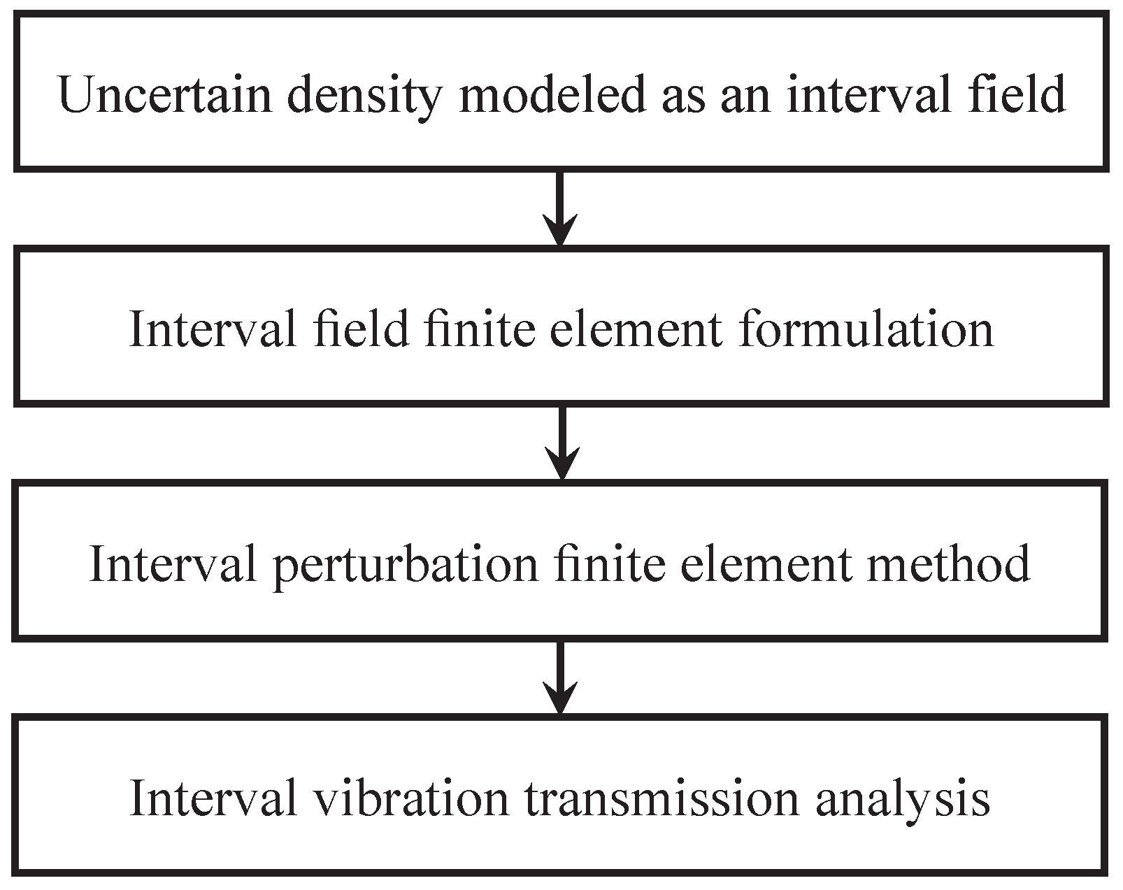
Figure 2.
Conventional MB structure.
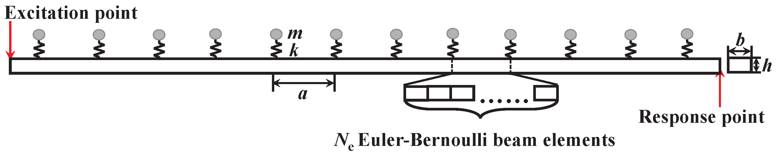
Figure 3.
Coordinate diagram of the basic beam’s finite element meshing.

Figure 4.
Vibration transmission of a finite MB.
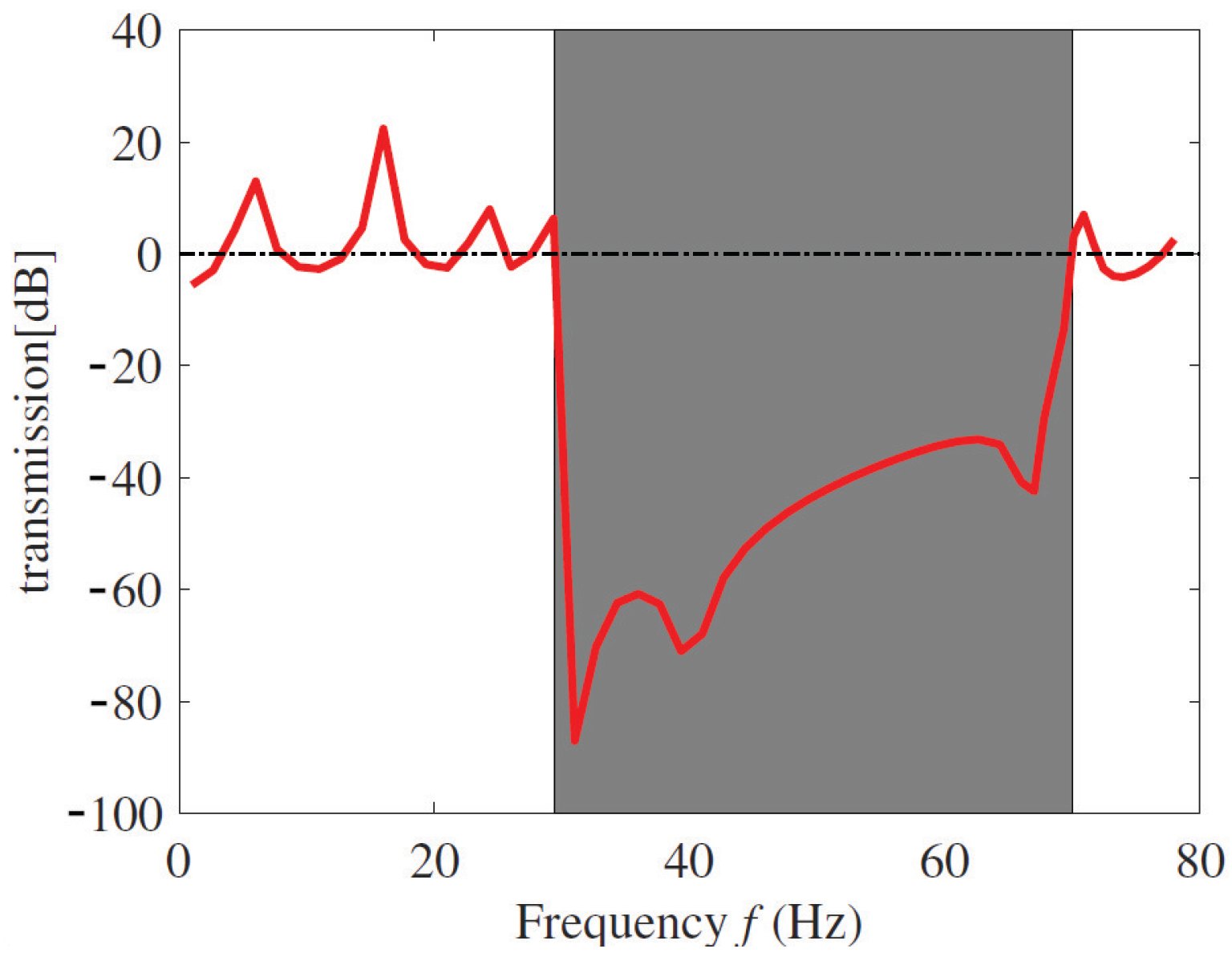
Figure 5.
IVTA of MB with interval density field ().
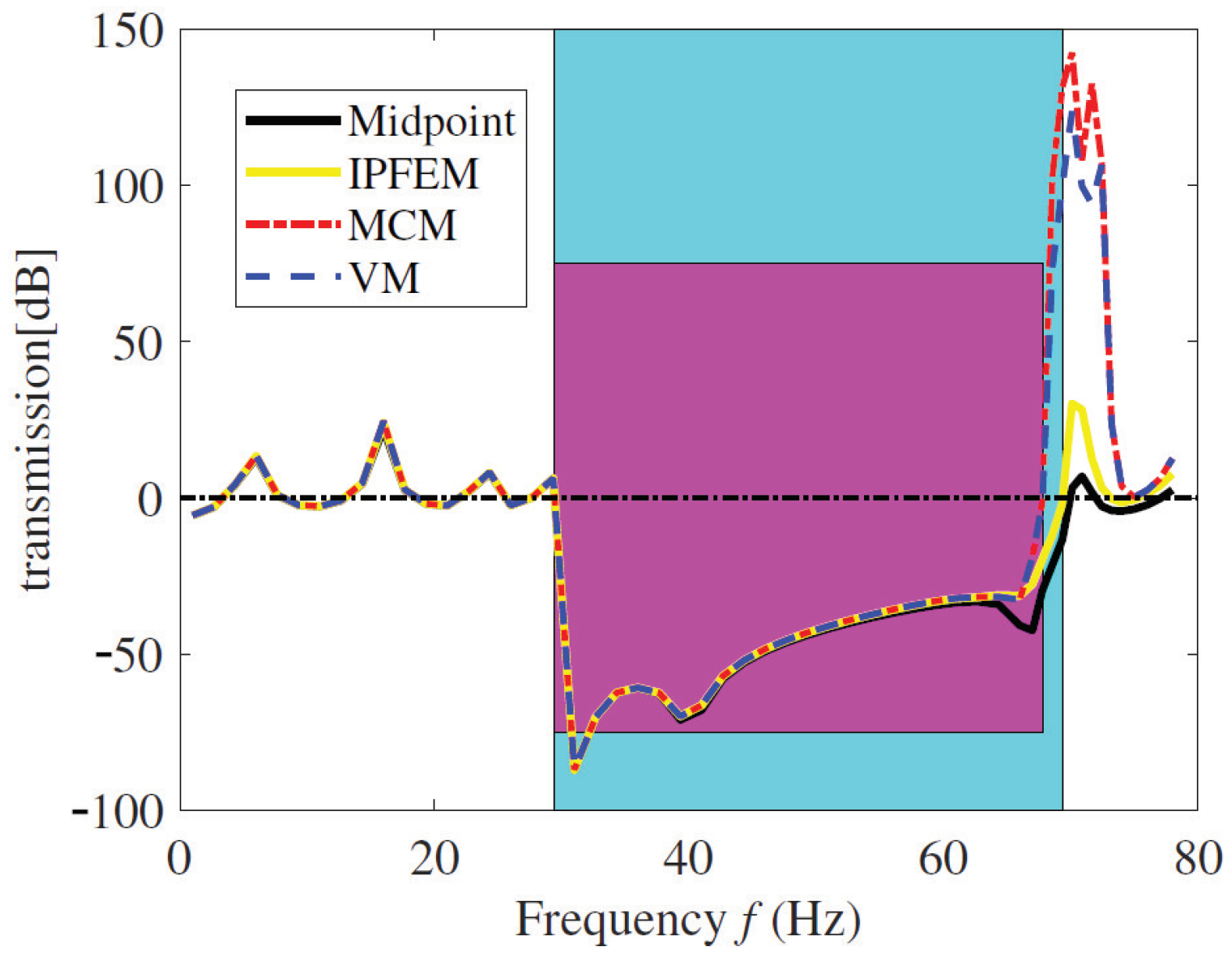
Figure 6.
Influences of the number of terms in KL expansion N on the ending frequency of the safe band gap. (a) . (b) . (c) .
Figure 6.
Influences of the number of terms in KL expansion N on the ending frequency of the safe band gap. (a) . (b) . (c) .
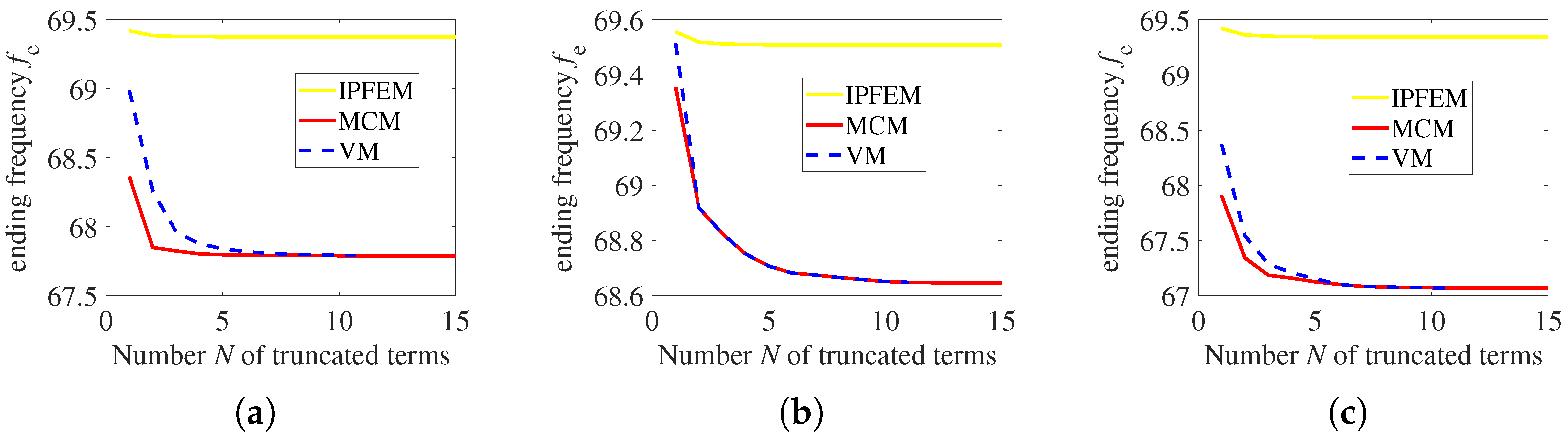
Figure 7.
Influences of interval field parameters on the ending frequency of the safe band gap. (a) Influences of . (b) Influences of .
Figure 7.
Influences of interval field parameters on the ending frequency of the safe band gap. (a) Influences of . (b) Influences of .
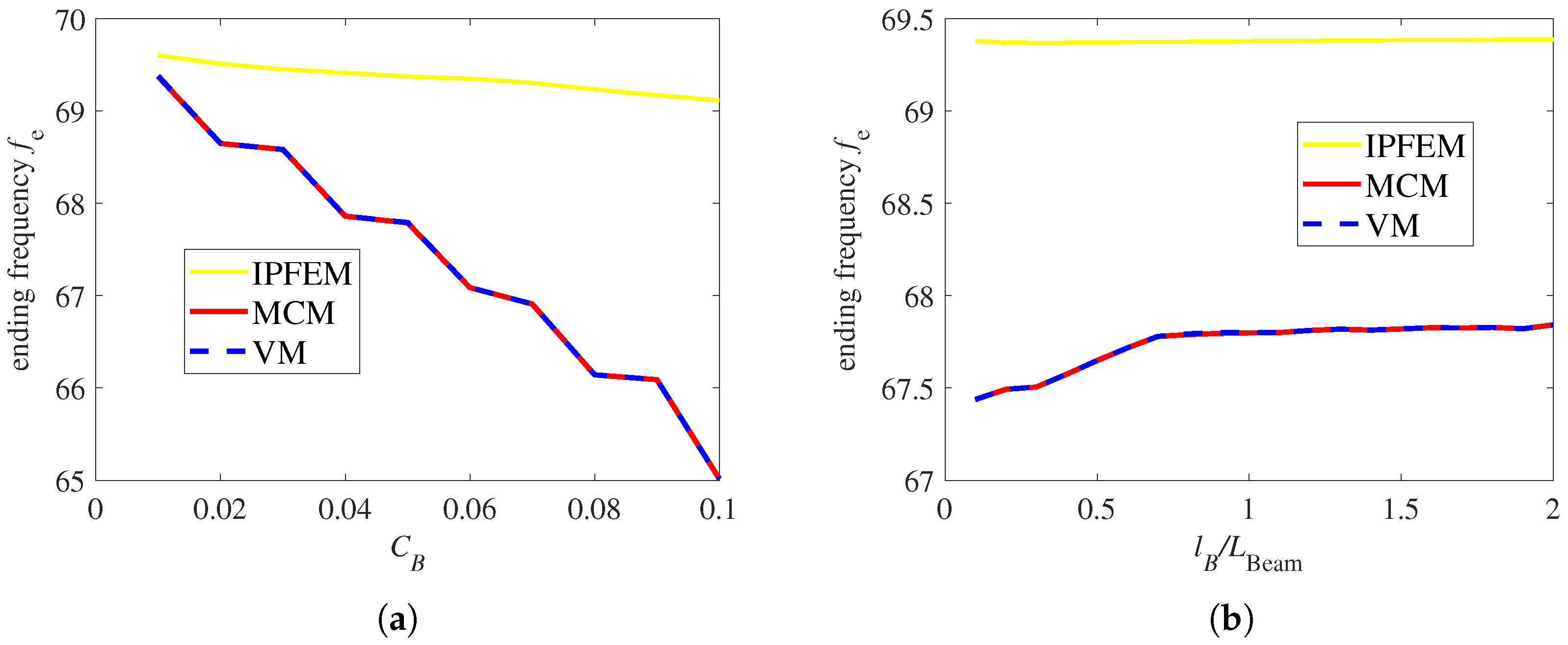
Figure 8.
Relative error of the ending frequency of the safe band gap according to IPFEM for different interval field parameters. (a) Different . (b) Different .
Figure 8.
Relative error of the ending frequency of the safe band gap according to IPFEM for different interval field parameters. (a) Different . (b) Different .
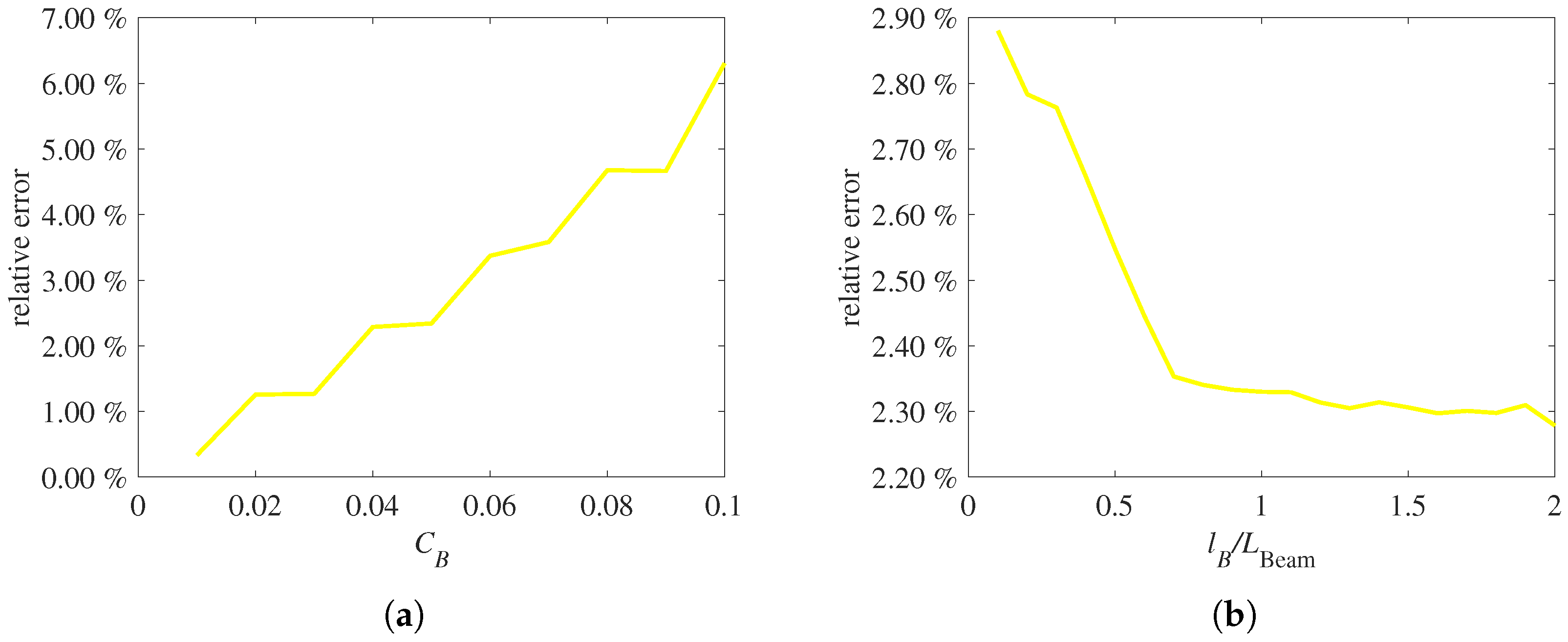
Figure 9.
IVTA of MB with interval density field () and interval resonator. (a) Interval resonator (). (b) Interval resonator ().
Figure 9.
IVTA of MB with interval density field () and interval resonator. (a) Interval resonator (). (b) Interval resonator ().

Disclaimer/Publisher’s Note: The statements, opinions and data contained in all publications are solely those of the individual author(s) and contributor(s) and not of MDPI and/or the editor(s). MDPI and/or the editor(s) disclaim responsibility for any injury to people or property resulting from any ideas, methods, instructions or products referred to in the content. |
© 2023 by the authors. Licensee MDPI, Basel, Switzerland. This article is an open access article distributed under the terms and conditions of the Creative Commons Attribution (CC BY) license (https://creativecommons.org/licenses/by/4.0/).
Share and Cite
MDPI and ACS Style
He, F.; Shi, Z.; Zhang, Z.; Qian, D.; Feng, X. Band Gap Properties in Metamaterial Beam with Spatially Varying Interval Uncertainties. Appl. Sci. 2023, 13, 8012. https://doi.org/10.3390/app13148012
AMA Style
He F, Shi Z, Zhang Z, Qian D, Feng X. Band Gap Properties in Metamaterial Beam with Spatially Varying Interval Uncertainties. Applied Sciences. 2023; 13(14):8012. https://doi.org/10.3390/app13148012
Chicago/Turabian StyleHe, Feiyang, Zhiyu Shi, Zexin Zhang, Denghui Qian, and Xuelei Feng. 2023. "Band Gap Properties in Metamaterial Beam with Spatially Varying Interval Uncertainties" Applied Sciences 13, no. 14: 8012. https://doi.org/10.3390/app13148012
Note that from the first issue of 2016, this journal uses article numbers instead of page numbers. See further details here.