The Statistical Error Optimization of Dye Sorption Equilibria for the Precise Prediction of Adsorption Isotherms on Activated Graphene

Abstract

The adsorption equilibrium of methyl blue (MB) at different temperatures was optimized using activated graphene (AG) as an adsorbent. The experimental data were compared using five linear and nonlinear adsorption isotherms, namely, Langmuir, Freundlich, Redlich–Peterson (R-P), Sips, and Toth, to estimate the best fit of the equilibrium data. Five distinct error functions were utilized to conduct nonlinear regression for the adsorption equilibrium: SSE, ARE, HYBRID, MPSD, and EABS. These functions offered a wide range of residuals for comparison. For a more accurate prediction of the isotherm model, two statistical techniques—SNE and CND—were applied. By using these techniques in conjunction, a more objective analysis of the error and deviation between the observed and predicted data was achieved, ultimately leading to improved accuracy in the error analysis. The sorption results demonstrated the highest MB removal of 691.89 mg g⁻¹, which amounted to 98.32% within 120 min. The error analysis findings indicated that the SSE and HYBRID functions produced the smallest error residuals. Based on the “goodness of fit” criterion, the models in this study were ranked as R-P > Toth > Langmuir > Sips > Freundlich. Among these models, the R-P isotherm demonstrated the best fit for the data, exhibiting the lowest variance in residuals. Its CND value ranged between 0.0025 and 0.0048, which further supports its superior fit compared to the other models. The combination of multiple error functions and statistical methods allowed for a comprehensive and objective assessment of the nonlinear regression models. The results highlight the importance of using various techniques to improve the accuracy of error analysis and identify the best-fitting isotherms for adsorption.

1. Introduction

Rapid civilization and industrial progress accelerate the continuous release of industrial waste into natural water streams. Waste from the cosmetics, paper making, food processing, and textile industries [1,2] is known to produce a number of hazards, with effluent dye pollution being one of the most significant [3,4]. Dyes are hazardous chemical constituents extensively used in the textile industry, and their discharge into water bodies can lead to the formation of toxic byproducts that persist for a long time and may cause respiratory problems, skin irritation, and even cancer [5,6]. Typically, MB has been identified as detrimental when released into water, affecting dissolved oxygen levels and harming aquatic life. Moreover, studies have demonstrated that MB dye can lead to various human health concerns due to its toxic nature, including skin irritation, allergic reactions, eye burns, and even cancer. Ingestion of the dye can also cause gastrointestinal distress, such as vomiting, diarrhea, and nausea. Given these risks, it is imperative to prioritize the complete removal or degradation of MB from discharge in open streams to promote sustainable ecology [7,8,9].

Diverse treatment techniques based on physical, chemical, and/or biological degradation have been developed to reduce the damaging effects of dyes on the environment [10,11,12,13]. Over the years, due to its low cost, straightforward operation, and effective remediation of pollutants, the adsorption process has been established as a well-recognized pollutant remediation technique. It has been widely used in various industries [14,15,16].

Activated carbon, zeolites, and agricultural wastes are being studied as adsorbents due to their moderate surface and porosity attributes, while graphene derivatives are emerging as promising alternatives due to their structural eminence, high efficiency, and low-cost feasibility. Moreover, graphene derivatives have exhibited excellent performance in removing heavy metals, organic pollutants, and dyes from wastewater [17,18,19,20]. They can also be easily modified to enhance their adsorption capacity and selectivity. However, to determine the sorption performance and capacity of an adsorption system under various experimental circumstances, the adsorption parameters must be understood and quantitatively compared. Since adsorption is a one-step process involving one or more physical and chemical phenomena of the adsorbate and adsorbent, an isotherm study is a straightforward approach to identifying the equilibrium conditions [21,22,23]. The isotherm study involves the determination of the type of isotherm model that best fits the experimental data to ensure an accurate prediction of the adsorption behavior. Additionally, understanding the equilibrium relationship between the adsorbent properties and the adsorption parameters is key for designing better adsorption systems for specific applications [9,24].

In most cases, the best-fit isotherm is determined using linear regression. However, researchers have concluded that linearizing adsorption isotherms usually changes the error structure of experimental data [24,25]. Moreover, the linearization of isotherms with three, four, and more parameters is not possible, as two or more unknown components limit simple linearization [26]. Nonlinear regression analysis provides a rigorous method of defining adsorption parameters using isotherm equations in their original form. It involves a stochastic distribution used to minimize the errors between experimental and simulated isotherm data [27]. Hence, a trial-and-error approach can be a solution used to minimize or maximize the objective function. However, this approach can be time-consuming and may not always guarantee the optimal solution. With the development of computer algorithms, this process has become faster, more reliable, and more efficient, allowing for quicker optimization of the objective function [28]. The statistical error functions are more reliable objective functions for the development and comparison of suitable nonlinear regression methods. To analyze the errors, a number of mathematically rigorous equations are used [28,29]. The sum of squared errors (SSE), the sum of absolute errors (SAE), the average relative error (ARE), the hybrid fractional error function (HYBRID), and Marquardt’s percent standard deviation (MPSD) are some of the most commonly cited regression functions used to search for best-fitting relationships in a solid–liquid adsorption system [30,31,32,33,34]. These regression functions yield different sets of residuals arising from different mechanisms [27]. To compare the residuals, numerous studies have reported on the standard normalizing process using the sum of normalized errors (SNE), as stated by Porter et al. [35,36,37,38]. In comparison, some other studies documented the selection of the optimal isotherm model based on the value of the highest R² and the lowest error function [4,39,40,41]. From a statistical perspective, although this proof of concept shows some quantitative relation among the error values, it cannot correlate with the variance of the residuals. Kumar et al. explained the accuracy of error analysis based on the coefficient of non-determination (CND) to identify the best-fit isotherm model [42]. The CND is a useful metric for measuring the proportion of variance in the dependent variable that is explained by the independent variables. Still, it does not provide information about the variability of the residuals around the fitted line. To fully improve the accuracy and reliability of model predictions, the combination of other statistical measures, such as the SNE, root mean square error (RMSE), average percentage error (APE), or mean absolute error (MAE), can be particularly useful for complex datasets, where feature selection is crucial for model performance.

In the present study, the equilibrium data of MB sorption on AG at four different test temperatures was computed using five linear and nonlinear adsorption isotherms, namely, Langmuir, Freundlich, Redlich–Peterson (R-P), Sips, and Toth. The underlying errors between the experimental and simulated isotherms were compared using five error functions, namely, the SSE, ARE, HYBRID, MPSD, and EABS. This offered a wide range of derived isotherm constants, making it challenging to determine the so-called optimal or the best-fitting relationship. Therefore, two different statistical methods, the SNE and CND, were used. The combination of these methods provided a more objective approach to quantifying the error and deviation between the observed and predicted data in different interpretations so as to compare the accuracy of the error analysis. Thus far, no studies combining ther SNE and CND to determine the best-fitting relationship with a detailed error analysis have been reported. Therefore, this study aims to fill this gap by proposing a novel approach that combines the SNE and CND methods to determine the best-fitting relationship with a comprehensive error analysis of dye sorption isotherms on various materials.

2. Experimental

2.1. Materials and Methods

The AG used as an adsorbent in this study is prepared from graphene oxide (GO). Typically, 10 mg of aqueous GO solution is successively stirred and ultrasonicated for 30 min and 1 h. Then, in an N₂ atmosphere, 5% NaBH₄ is slowly added and raised to a temperature of 200 °C for 12 h. Methyl blue (MB) is used as a sample pollutant adsorption indicator.

Table 1. Specifications of AG used as an adsorbent.

Particulars	Unit
Surface area	589.06 m2 g−1
Average pore size	4.49 nm
Pore volume	5.62 × 10−1 cm3 g−1
Crystal size	4.49 Å
Crystallite lattice sizes	15 nm
C	88.13%
O	11.5%
N	0.37%

lists the physical and chemical properties that were determined using standard procedures [9]. The details of the chemicals used are provided in Supplementary Table S1.

2.2. Batch Adsorption

The batch adsorption of MB is carried out by adding 0.005 g AG with 30 mL dye solution (conc. 50 mg/L) of a predefined primary concentration at four different solution temperatures of 303, 313, 323, and 333 K. After 12 h of the retention time, which is sufficient to reach equilibrium, 2 mL of the solution is systematically added to 3 mL of DI water before the UV-vis analysis. A 0.45 µm PVDF membrane is then used to filter the supernatant. The dye’s equilibrium concentration (C_e) is determined through spectral analysis. In contrast, the dye separation% is estimated using Equation (1), and the sorption capacity (q_e) of the adsorbent at equilibrium is measured using Equation (2):

$$S\%=\frac{C_0-C_e}{C_0}\times 100$$

(1)

$$q_e=\frac{C_0-C_e}{m}\times V$$

(2)

Here, C₀ and C_e denote the initial and equilibrium concentrations, respectively; m and V stand for the adsorbent mass and volume of the solute adsorbate, respectively.

2.3. Isotherm Model Fitting

Adsorption isotherm model fitting using either theoretical or empirical equations is a practical way to design and operate an adsorption system. MB dye sorption via AG was carried out by establishing a fitting correlation of the equilibrium curve. In this context, typical two-parameter isotherm models, namely, the Langmuir and Freundlich models, and three-parameter-based models, namely, the R-P, Sips, and Toth models, were tested linearly and non-linearly to construct a fitting correlation through comparison. We aimed to determine the least significant deviation from the model fitting to the experimental data for a best-fit equation of the isotherm parameters. The corresponding linear and nonlinear model forms, plotting techniques, and parameters are presented in

Table 2. The linear and nonlinear forms of isotherm models and their parameters.

Model	Nonlinear	Linear	Linear Plot	Parameters
Langmuir	$q_e=\frac{k_L{q}_m{C}_e}{1+k_L{C}_e}$	Type-1 $\frac{1}{q_e}=\frac{1}{K_L{q}_m{C}_e}+\frac{1}{q_m}$	$\frac{1}{q_e}$ vs. $\frac{1}{C_e}$	KL, qm
		Type-2 $\frac{1}{C_e}=\frac{K_L{q}_m}{q_e}-K_L$	$\frac{1}{C_e}$ vs. $\frac{1}{q_e}$
		Type-3 $q_e=q_m-\frac{q_e}{K_L{C}_e}$	qe vs. $\frac{q_e}{C_e}$
		Type-4 $\frac{q_e}{C_e}=K_L{q}_m-K_L{q}_e$	$\frac{q_e}{C_e}$ vs. $q_e$
		Type-5 $\frac{C_e}{q_e}=\frac{C_e}{q_m}+\frac{1}{K_L{q}_m}$	$\frac{C_e}{q_e}$$\mathrm{vs}.C_e$
		Type-6 $C_e=q_m\frac{C_e}{q_e}-\frac{1}{K_L}$	Ce vs. $\frac{C_e}{q_e}$
Freundlich	$q_e=k_f{C}_e^{\frac{1}{n}}$	$Ln{K}_f+\frac{1}{n}Ln{C}_e$	Lnqe vs. LnCe	KF, n
R-P	$q_e=\frac{A{C}_e}{1+B{C}_e^g}$	$ln\left(A\frac{C_e}{q_e}-1\right)=gln\left(C_e\right)-ln\left(B\right)$	$ln\left(A\frac{C_e}{q_e}-1\right)\mathrm{vs}. ln\left(C_e\right)$	A, B, g
Sips	$q_e=\frac{q_m{b}_s{c}_e^{\raisebox{1ex}{$1$}\!\left/ \!\raisebox{-1ex}{$n$}\right.}}{1+b_s{c}_e^{\raisebox{1ex}{$1$}\!\left/ \!\raisebox{-1ex}{$n$}\right.}}$	$ln\left(\frac{q_e}{q_m-q_e}\right)=\frac{1}{n}ln\left(C_e\right)+ln{\left(b_s\right)}^{\raisebox{1ex}{$1$}\!\left/ \!\raisebox{-1ex}{$n$}\right.}$	$ln\left(\frac{q_e}{q_m-q_e}\right)\mathrm{vs}.ln{c}_e$	qm, bs, n
Toth	$q_e=\frac{q_m{K}_T{C}_e}{\left[1+\left(K{C}_e\right)n\right]\raisebox{1ex}{$1$}\!\left/ \!\raisebox{-1ex}{$n$}\right.}$	$ln\left(\frac{q_e}{q_m-q_e}\right)=nln{K}_T+nln\left(C_e\right)$	$ln\left(\frac{q_e}{q_m-q_e}\right)\mathrm{vs}.ln\left(C_e\right)$	qm, KT, n

[6,43].

3. Results and Discussion

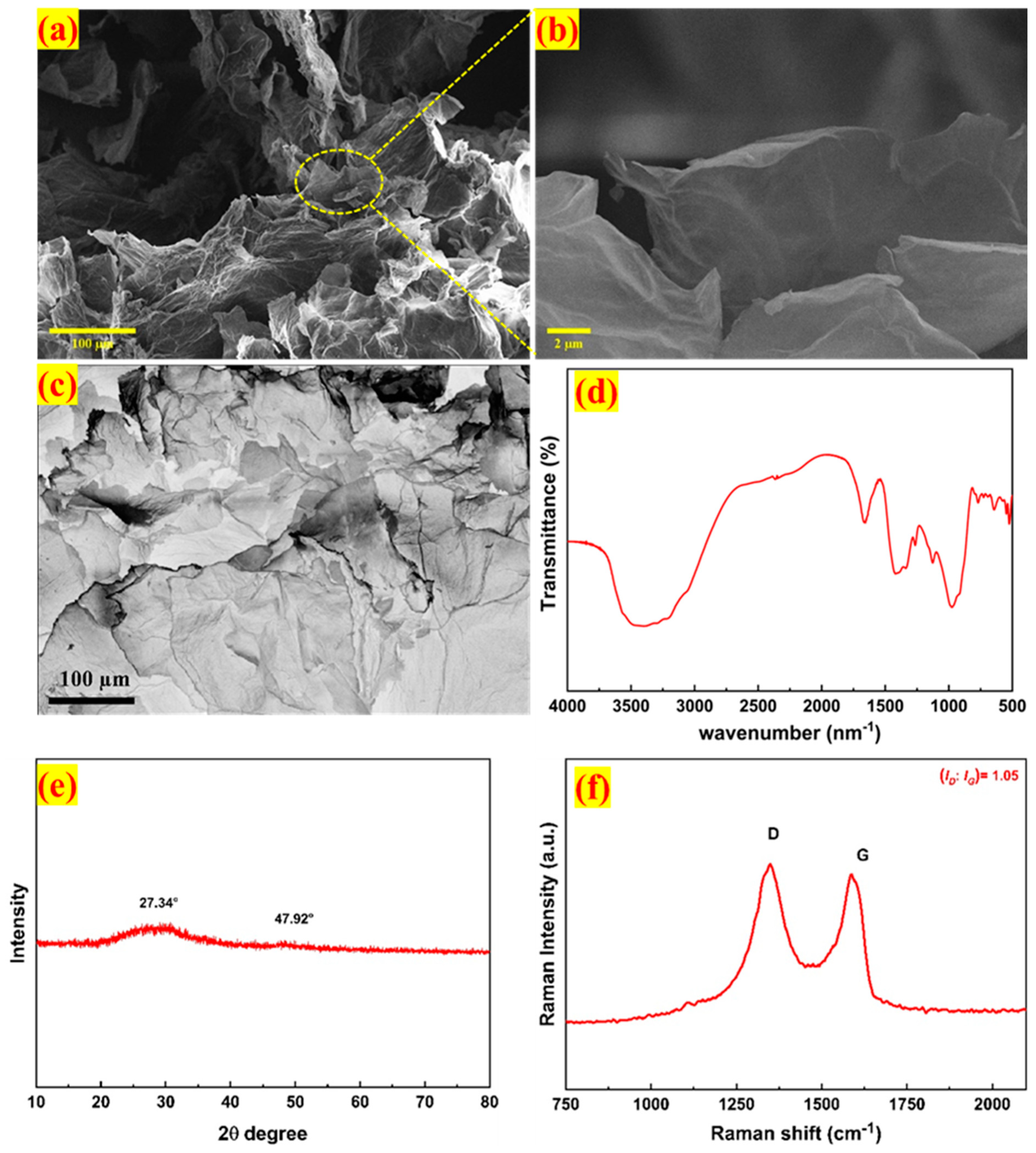
3.1. Material Characterization

Field-emission scanning electron microscopy (FE-SEM) using an ULTRA 55 instrument from Carl Zeiss AG, Germany, was employed to study the microstructures and morphology of the samples under vacuum conditions at an accelerating voltage of 20 kV. Before examination, the samples were mounted on carbon-based adhesive tape and coated with a 2 nm thick platinum layer. The SEM image (Figure 1a) displays a significant number of wrinkles and corrugations on the graphene’s basal plane, while its fluffy appearance indicates the expansion of inter-sheet packs within numerous carbon layers due to exfoliation [44,45,46]. At a higher magnification (Figure 1b), irregular flakes are observed, which are intertwined due to the cohesive force from the π–π stacking of sp3 hybridized carbon atoms. Additionally, the pseudo-color topographic contrast of the SEM image from Mountains^® surface profiling, Digital Surf, SA. Besançon, France https://www.digitalsurf.com/ (accessed on 10 September 2022) (Figure 1c), reveals that the combination of chemical and thermal treatments produced a thin, paper-like material with an extensive surface area and porous channels [47]. Fourier transform infrared (FTIR) spectroscopy (Nicolet IS-50, Thermo Scientific, Waltham, MA, USA) of the sample demonstrated the presence of several oxygen-containing functional groups, such as C-O, C-OH, and C-O-C, at 1658, 1415, and 1125 nm⁻¹, respectively (Figure 1d) [48]. The low intensity of these bands indicates that thermal treatment has induced graphitization within the carbon framework [49]. The strong, broad band at 3450 cm⁻¹ confirms the presence of carboxylic functional groups [50]. As expected, the sample has a high carbon content, which is crucial for determining the bonding nature. Furthermore, the combination of chemical and thermal treatments disrupts the structural arrangement and introduces defects, leading to the deconvolution of the C-O and O-C-O bonds [51]. X-ray diffraction (XRD) analysis (D8 Advance, Bruker Corp., Billerica, MA, USA) of the sample revealed a broad peak at 27.34°, indicative of graphitization, which corresponds to an interplanar spacing of 3.7 Å (Figure 1e) [52]. An additional peak at 47.92°, associated with the (100) plane, suggests the formation of flake-like structures with crystal sizes less than or equal to 1 nm. Raman spectroscopy (In-Via confocal, Renishaw plc., Wotton-under-Edge, UK) was further performed to investigate the samples’ structural features, such as their intrinsic structural disorder (I_D/I_G ratio) and crystallite lattice size (L_a) (Figure 1f) [53]. The typical D and G bands were observed at 1350 and 1586 cm⁻¹, respectively, as the defect-inducing chemical exfoliation provided reactive sites within the sample [54]. Consequently, the high I_D/I_G ratio of 1.05 is consistent with the chemical exfoliation process, yielding a crystallite lattice size (L_a) of 15 nm [55].

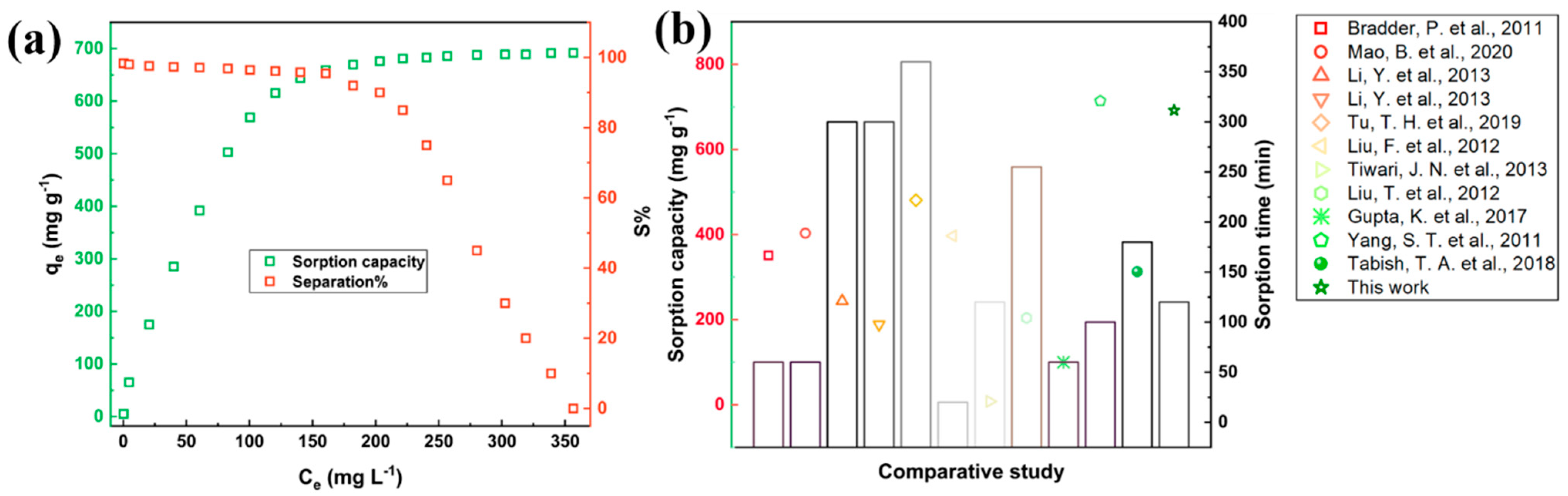
3.2. Adsorption Study

The adsorption of MB was assessed through UV-vis spectral analysis, with the maximum sorption capacity at equilibrium and the dye separation percentage being calculated as per Equations (1) and (2). The data obtained are plotted in Figure 2a. It is clear from Figure 2a that the adsorption capacity (q_e) increases rapidly at a lower equilibrium concentration (C_e). At a C_e of 150 mg L⁻¹, the maximum qe exceeded 650 mg g⁻¹, achieving a removal efficiency greater than 97% within 80 min. However, once a saturation peak was reached, the sorption process leveled off, with only minimal additional adsorption observed. The maximum sorption capacity attained was 691.89 mg g⁻¹, equating to a 98.32% removal rate within 120 min. It is anticipated that the microstructure morphology of the adsorbent drove the adsorption process. The presence of numerous reactive carbonaceous groups (epoxy, hydroxyl, carboxylic, and phenolic) in the AG facilitated an electrostatic interaction with the dye’s mass center. As a result, the AG demonstrated superior adsorption compared to the other similar graphene family materials (as shown in Figure 2b) (relevant data detailed in Supplementary Table S3). The skeleton structures of these materials are nearly identical and likely to exhibit some degree of π-π stacking interaction. However, higher levels of oxygen functionalities may result in a lower affinity for the dye molecules, leading to either reduced adsorption or an extended time needed to achieve equilibrium.

3.3. Linear Fitting

Linear regression is the most common isotherm fitting technique that uses the linear least-squares method. It provides structurally evolving isotherm equations for straightforward experimental data fitting using the coefficient of determinant. The linearization approach of the Langmuir isotherm model allows for data fitting through the six different forms of simple linear regression for various parameters. The plotting techniques of the linearized forms that are used to estimate q_m and K_L are given in Table 2. Interestingly, the linear models obtained have pairs due to the analogous iterative interexchange of variables (Table 2). The corresponding “Type-1 & 2, Type-3 & 4, and Type-5 & 6” result from the interchange of independent and dependent variables during the linearization of the governing equation (Figure S1) [22]. Theoretically, it is assumed that the independent variable is error-free, as it is the experimental entity. However, relocating the numerator and denominator for regression may alter the correlation results. Therefore, deviations in the different parameters of a fitted equation enable one to search for the best error distribution through comparison. All five models’ linear fit isotherm parameters, including the data obtained from the six linear-transformed Langmuir models, are documented in

Table 3. Data obtained from linear-fitted isotherm models (units, q_max: mg g⁻¹, K_L: L mg⁻¹, K_F: (mg g⁻¹) (L g⁻¹) ⁿ, b_s: L g⁻¹, B: L mg⁻¹, A: L g⁻¹).

Models	Parameters	Temperature (K)
		303	313	323	333
Langmuir Type-1	qmax	660.491	766.344	721.527	727.711
	KL	0.027	0.025	0.033	0.037
	R2	0.999	0.999	0.999	0.999
Langmuir Type-2	qmax	661.636	766.768	722.122	728.578
	KL	0.027	0.025	0.033	0.037
	R2	0.999	0.999	0.999	0.999
Langmuir Type-3	qmax	810.821	797.165	807.475	828.349
	KL	0.0194	0.023	0.026	0.029
	R2	0.889	0.915	0.888	0.884
Langmuir Type-4	qmax	844.915	820.192	837.234	858.515
	KL	0.017	0.021	0.023	0.025
	R2	0.889	0.915	0.888	0.884
Langmuir Type-5	qmax	820.772	801.373	816.299	851.26
	KL	0.019	0.023	0.026	0.026
	R2	0.990	0.993	0.991	0.993
Langmuir Type-6	qmax	812.614	796.02	855.012	845.473
	KL	0.019	0.024	0.021	0.027
	R2	0.990	0.993	0.991	0.993
Freundlich	1/n	0.666	0.642	0.623	0.612
	KF	19.509	22.705	26.035	28.779
	R2	0.956	0.942	0.943	0.944
Sips	qm	691.9	696.456	714.864	748.873
	n	0.996	0.991	0.99	1.001
	bs	0.019	0.023	0.026	0.027
	R2	0.985	0.986	0.977	0.982
R-P	g	0.737	1.073	0.837	0.814
	B	0.096	0.017	0.071	0.09
	A	18.67	19.09	23.9	27.39
	R2	0.987	0.98	0.99	0.991
Toth	qm	692.907	700.333	716.741	749.844
	n	1.004	1.009	1.01	0.999
	KT	0.019	0.023	0.026	0.027
	R2	0.985	0.986	0.977	0.982

, and the fitted curves are shown in Figure 3. Table 3 shows that the Langmuir isotherm parameters differ from each other in terms of the linear forms. Among the six Langmuir models, Type-1 and Type-2 give the highest R² values for all measured temperatures [25]. Meanwhile, these two forms have a lower maximum adsorption capacity (q_m) than the others. These effects result from the methods adopted for extrapolating the isotherm model’s linearization, where the error distribution either conforms or deflects.

On the other hand, the Type-4 Langmuir model form has the highest q_m, amounting to 844.9 mg g⁻¹, with a low R² value (the same as Type-3). From Table 2, we can see that at 333 K (Type-4), the highest q_m of 858.515 mg g⁻¹ for MB sorption was found. However, dissimilarity in the Langmuir constant (K_L) and a lower coefficient for particular temperatures are observed due to the equations with a structurally varying error distribution.

The low R² from the linear fitting of the Freundlich isotherm (Table 3) and scatter from the experimental data (Figure 3) for all temperatures show the poor fitting in the present study. Therefore, the equilibrium data obtained through MB adsorption on the AG were fitted in the linearized form of three-parameter isotherm models, namely, R-P, Sips, and Toth. Due to three unknown digits, the traditional linearization of this model was not possible. Hence, trial-and-error minimization based on computer operating techniques was applied.

The R-P isotherm, after linear transformation, was plotted against $ln\left(A\frac{C_e}{q_e}-1\right)\mathrm{vs}. ln\left(C_e\right)$. Since it is a hybrid isotherm generated by combining Langmuir and Freundlich models, each parameter, including A, B, and g, refers to an empirical condition. Here, the exponent g signifies the nature of the adsorbent and can explain the adsorption process to an extent. Within the boundary of 0–1, if the g value tends towards 0, one presumes that the heterogeneous surface nature of the adsorbent is related to Freundlich-type adsorption and vice versa. The calculation of the unknown parameters is simplified by maximizing the coefficient R² between the maximum adsorption data q_e and the values calculated from the linearized R-P isotherm equation. In Table 2, the R² value for all four temperatures is 0.987–0.991, which is higher than the data obtained for the Freundlich isotherm’s linear fitting. Consequently, the g values for all four temperatures are close to 1 in the R-P equation, implying a Langmuir-type mechanism.

Similar to the R-P isotherm, the Sips and Toth isotherm models combine the Langmuir and Freundlich models. However, each model has distinctive characteristic features. Typically, the Sips model predicts heterogeneous surface adsorption and circumvents the limitation observed at a high adsorbate concentration in the Freundlich model. Thus, the model predicts heterogeneous surface adsorption at low adsorbate concentrations, while it assumes monolayer adsorption at higher concentrations. The model’s parameters are also subject to pH, temperature, and concentration.

In comparison, the Toth isotherm model is suitable for identifying heterogeneous adsorption systems in an adsorbate’s low- and high-concentration boundary conditions. Additionally, it considers the adsorbent surface’s heterogeneity, and the exponent n characterizes the heterogenicity of the adsorption system. If n is between 0 and 1, the model follows the Langmuir equation; however, in the heterogeneous adsorption system, n deviates from unity (1). The data obtained from the Sips and Toth models based on linear fitting at all four temperatures are presented in Table 3. The empirical data tend to have an identical coefficient for every testing temperature, indicating the Toth model’s superiority over the Sips model [6]. Table 3 shows that the R² values of the two models are the same for a particular temperature. Except for 333 K, the values of n for the AG are slightly higher than 1 in all of the studied temperatures for MB adsorption, suggesting the systems’ heterogeneity and providing support for the Freundlich model. Similar to the Sips model, the Toth isotherm equation also implies the involvement of heterogeneous adsorption for the consecutively lower temperatures of 303–323 K as n ≤ 1.

Meanwhile, the monolayer adsorption capacity predicted with the Sips and Toth models follows similar trends to the Langmuir equation. Thus, the comparison of the values of R² and the other parameters of all six linearized Langmuir equations with those of the Freundlich, R-P, Sips, and Toth isotherms shows different outcomes. Figure 3a–d shows the linear regression of the predicted isotherms against the experimental equilibrium data at 305, 313, 323, and 333 K, respectively. From Figure 3, it is evident that the linearized isotherms do not fit well with the experimental equilibrium data. This results from the data transformations that violate least-squares normality assumptions and indirectly change the error structure and the error variance [66].

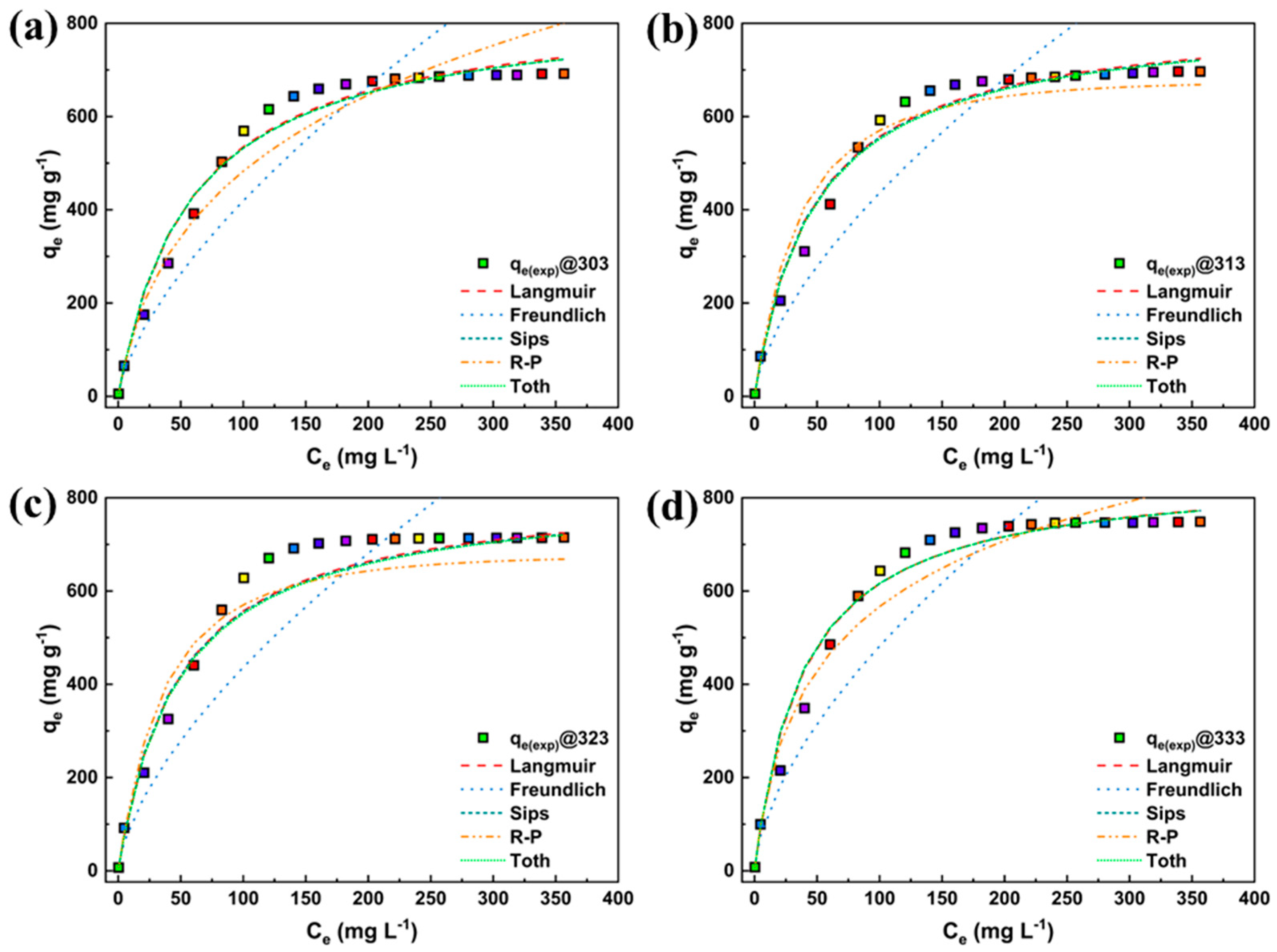
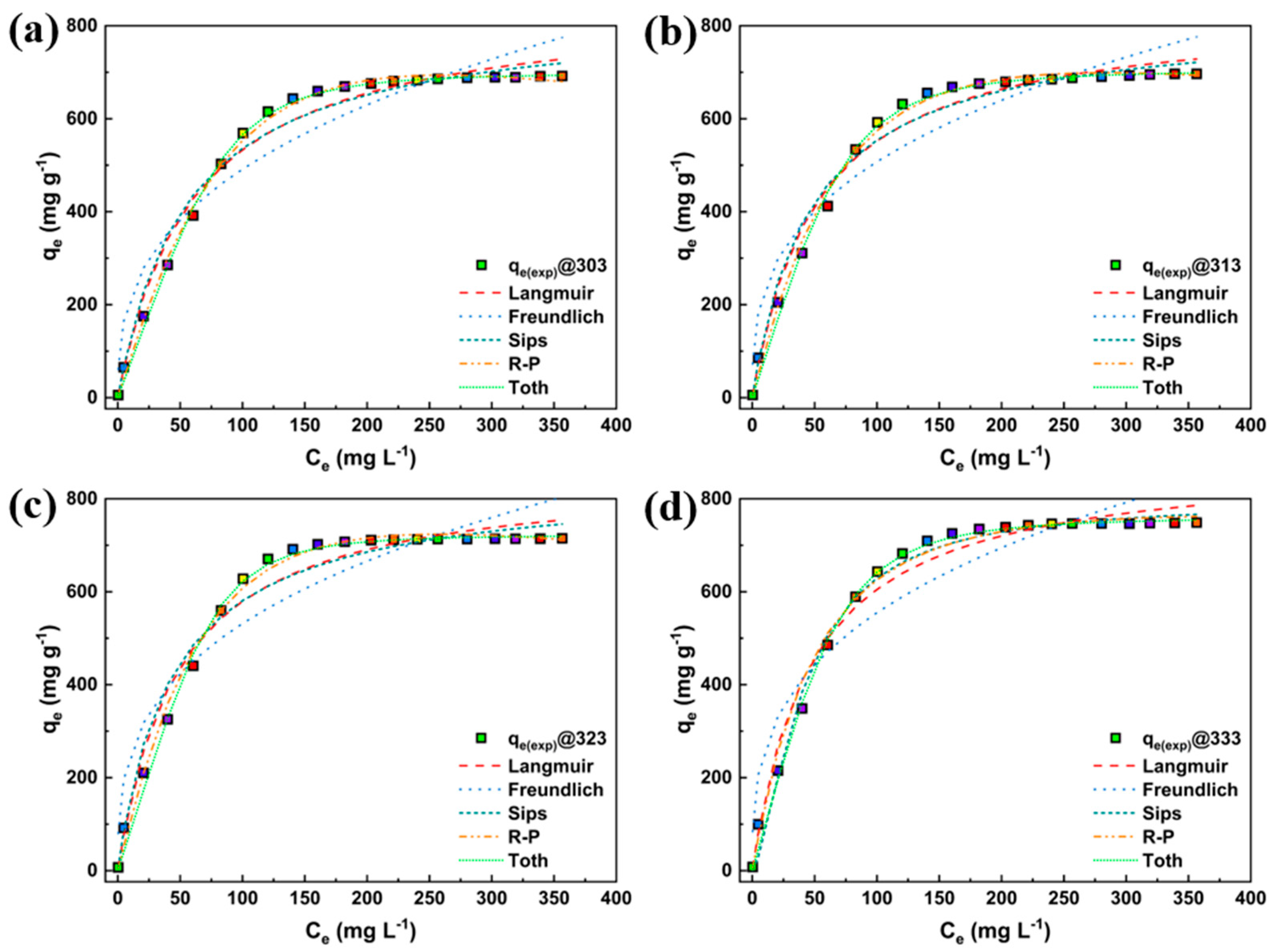
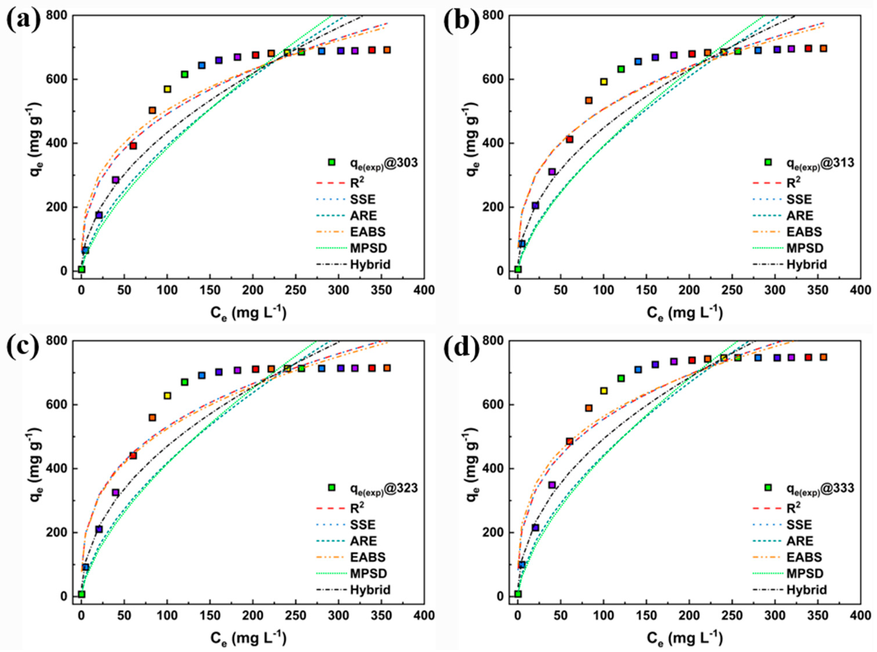
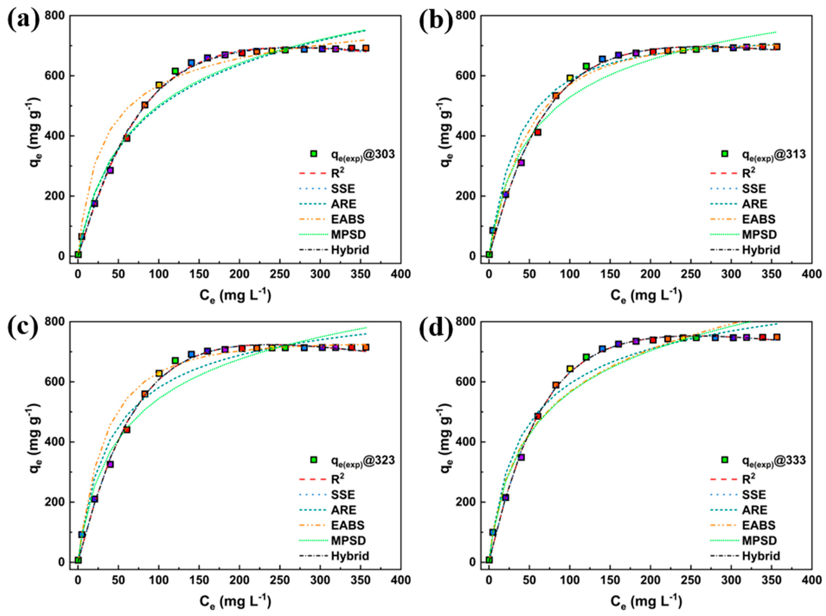
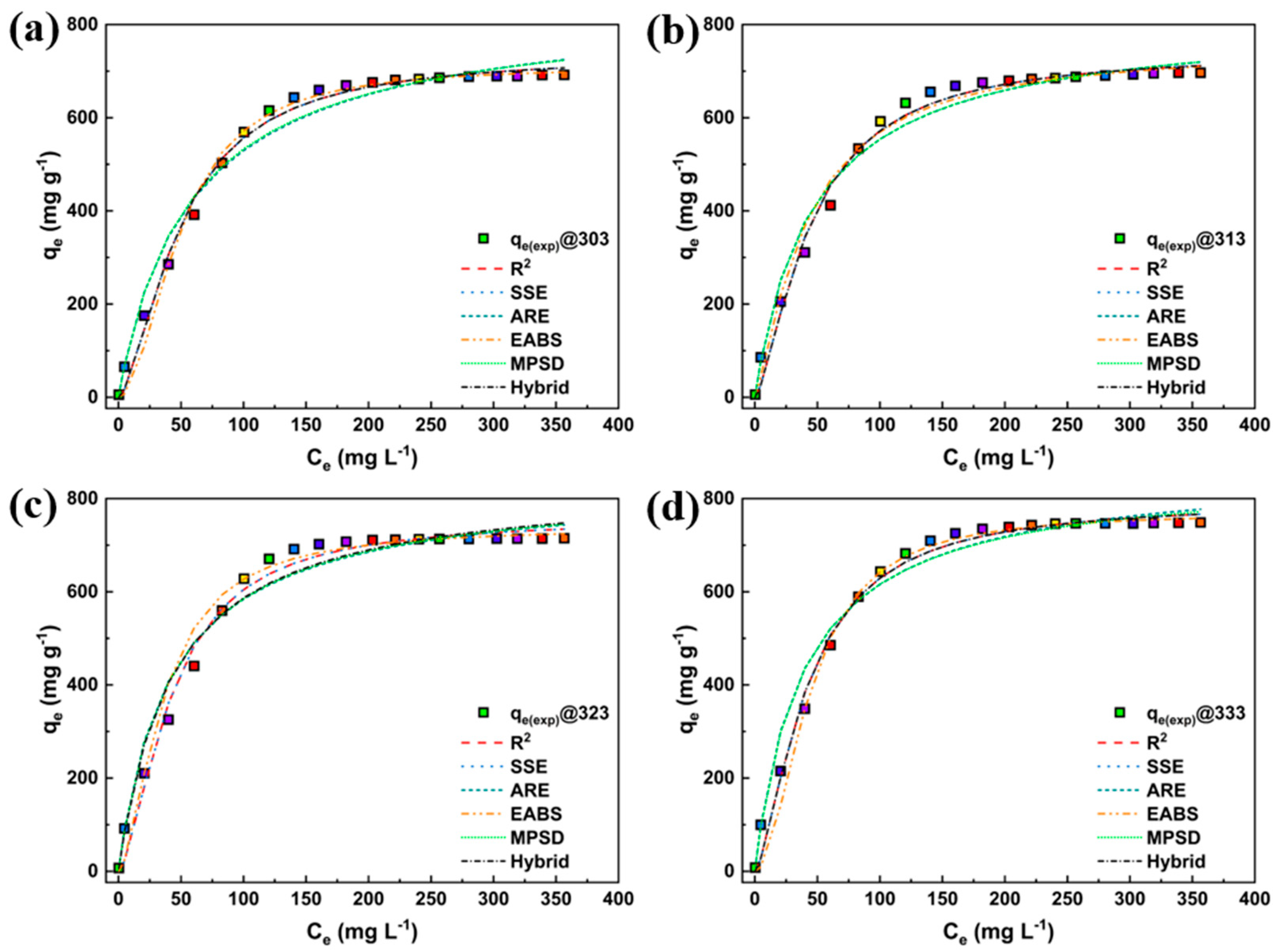
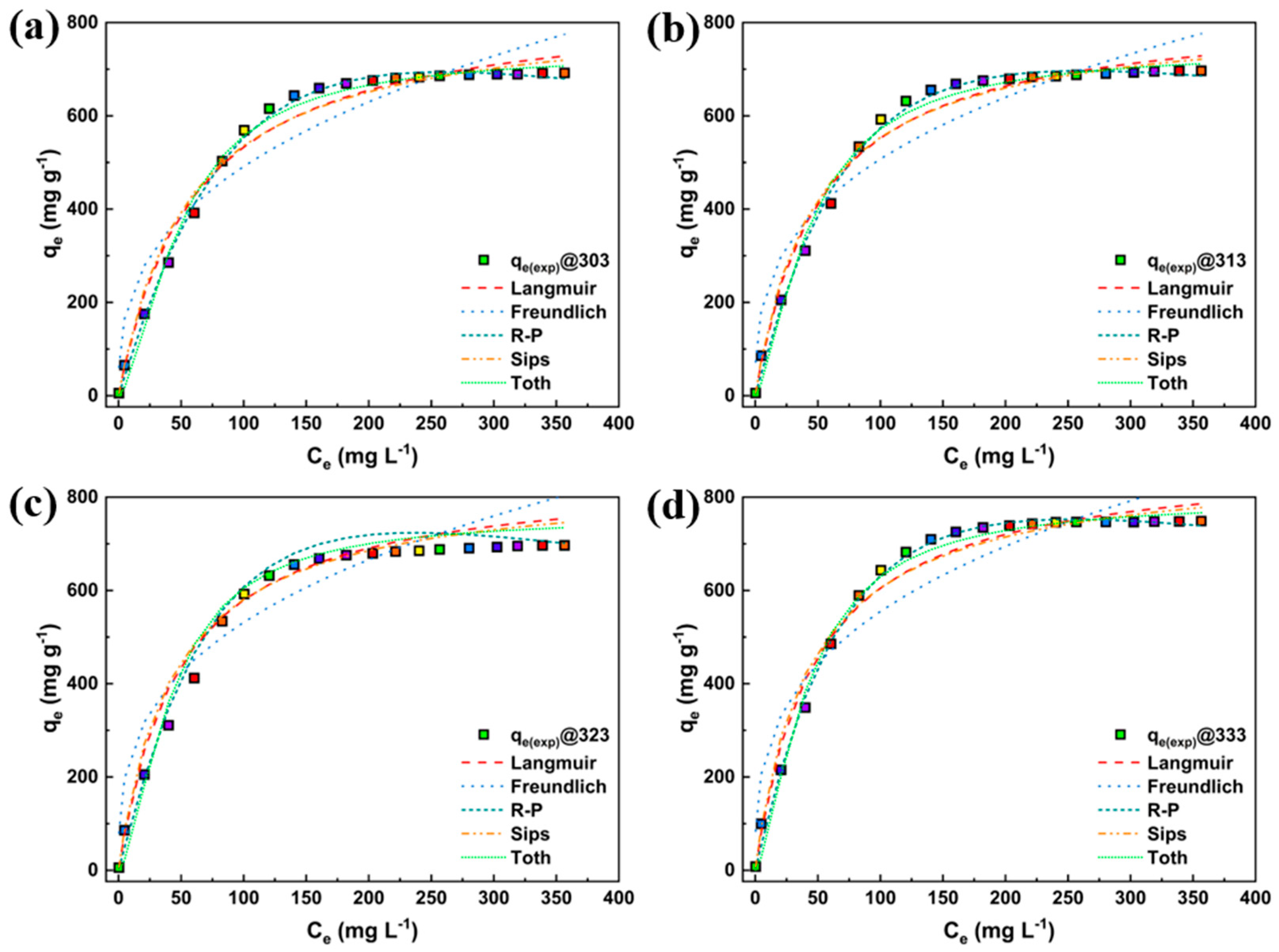
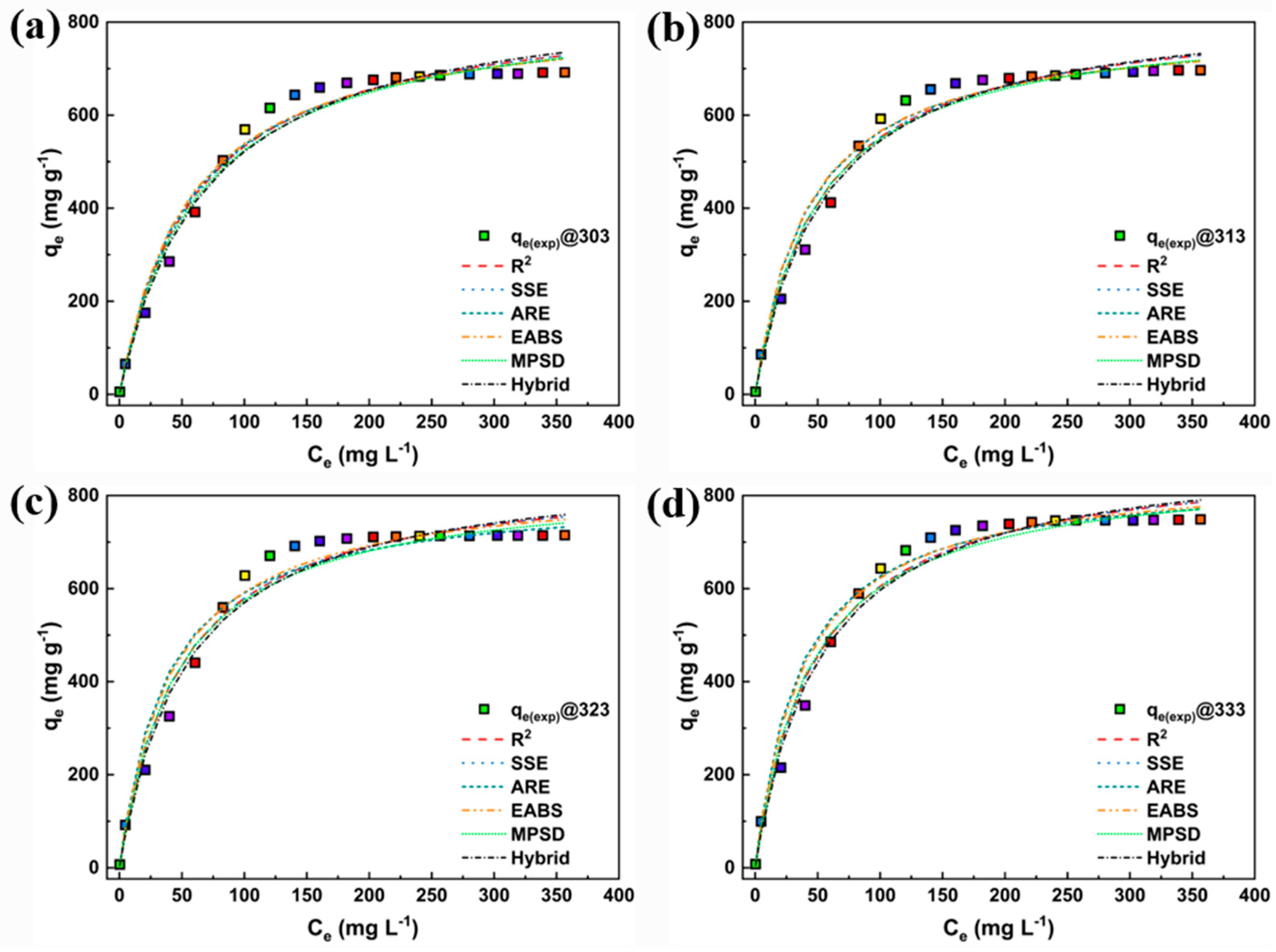
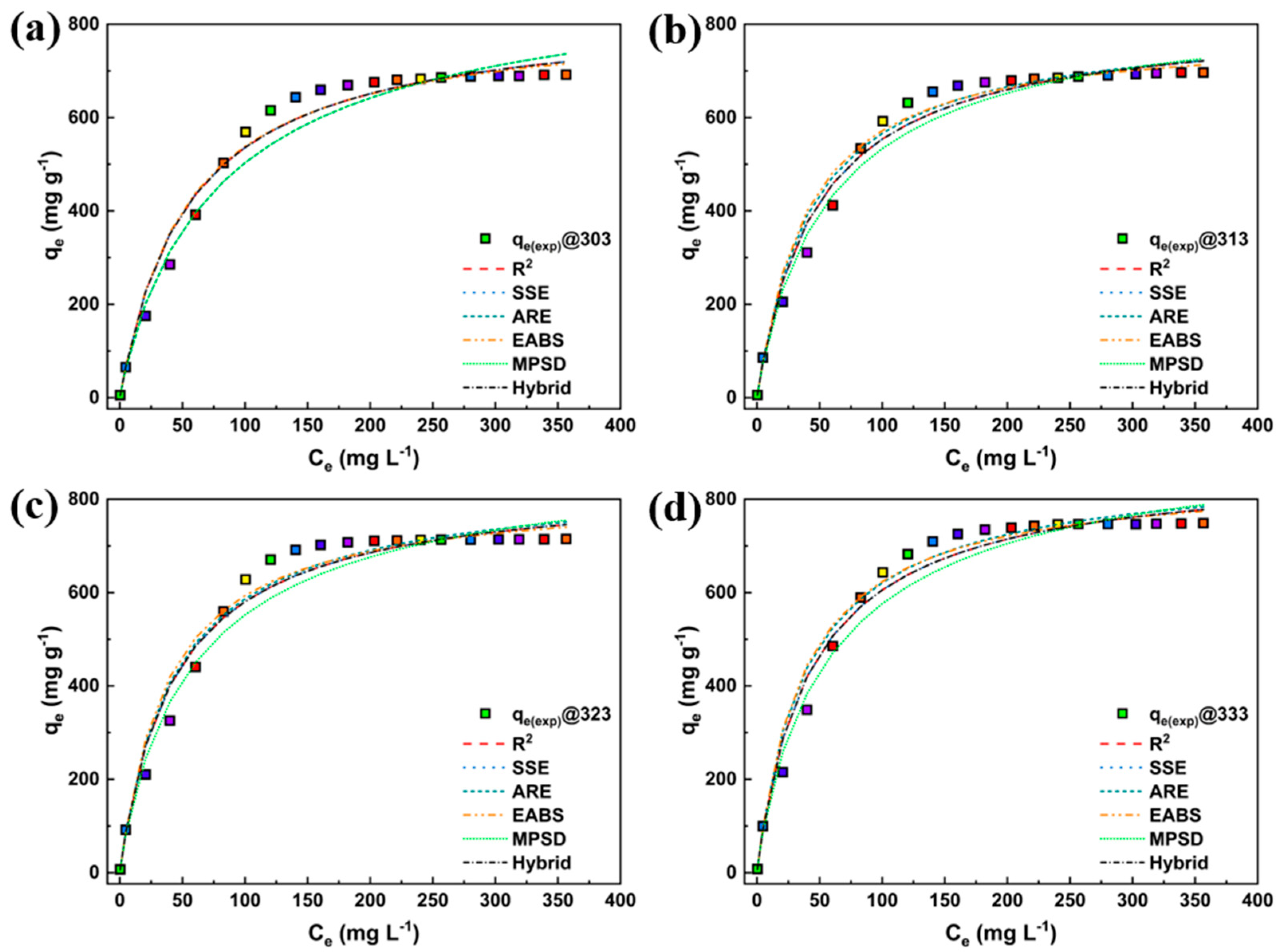
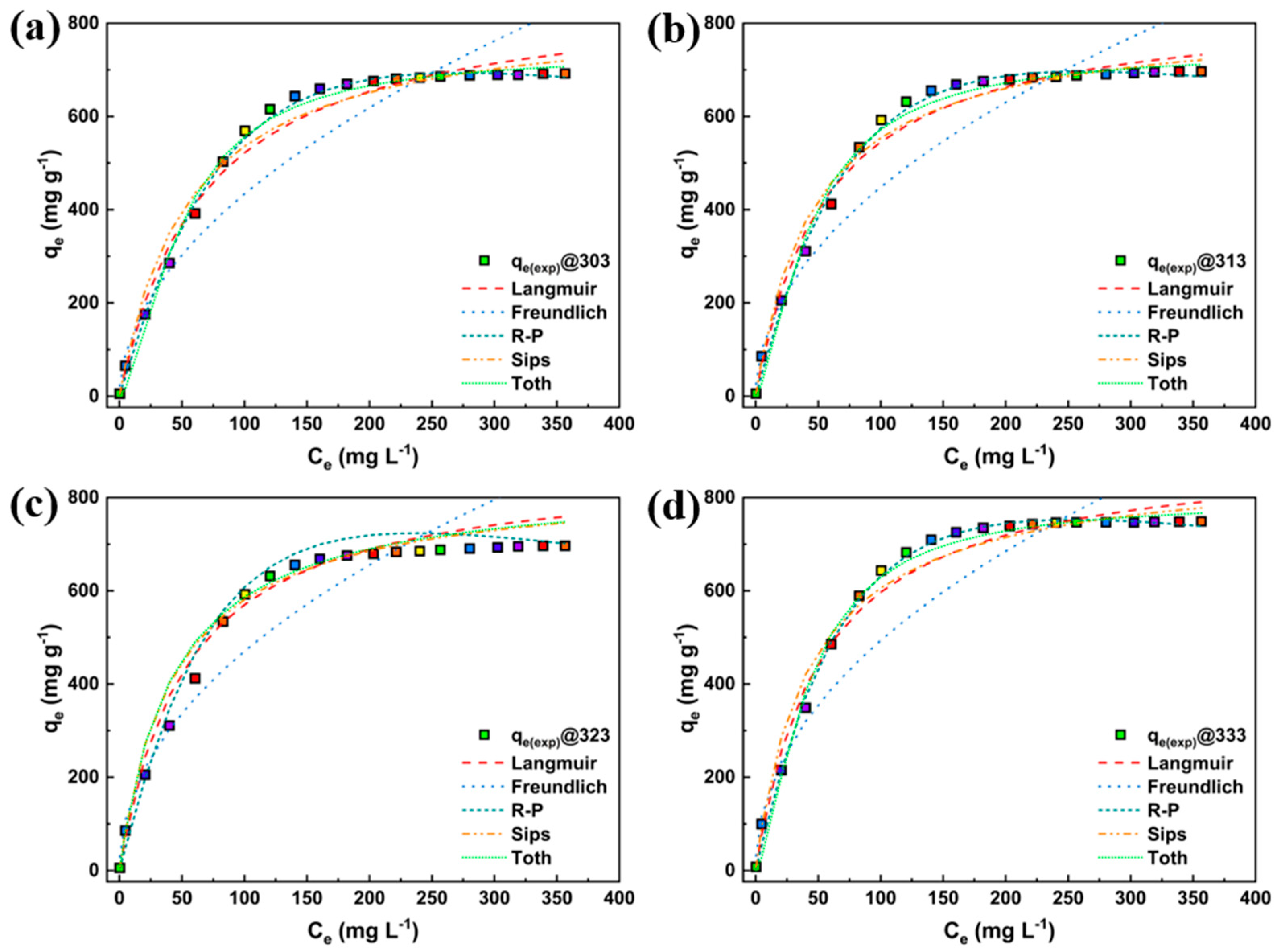
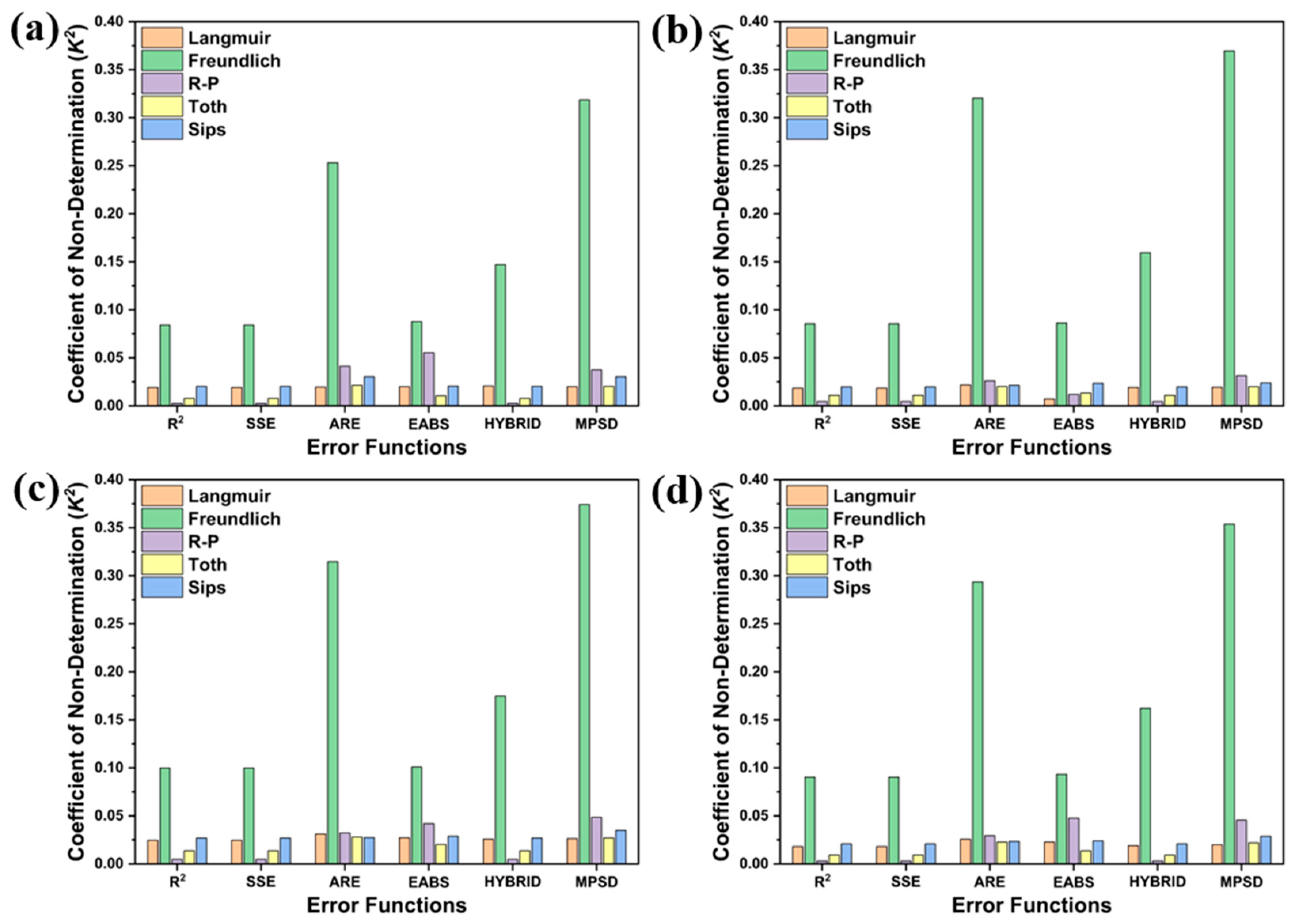
3.4. Nonlinear Fitting

The nonlinear method is a draft process in which a trial-and-error action is functional under the testing conditions. With contemporary technological progress, the processing of nonlinear regression has become effective using computer-based solving features. The present study was carried out to perform nonlinear data fitting through Microsoft Excel’s solver add-in with a spreadsheet. The curve fitting results for the experimental and predicted equilibrium data of all five isotherm models using nonlinear methods at consecutive temperatures of 303–333 K are shown in Figure 4, and the parameters obtained from the nonlinear forms are included in

Table 4. Data obtained from nonlinear isotherm model fitting (units, q_max: mg g⁻¹, K_L: L mg⁻¹, K_F: (mg g⁻¹) (L g⁻¹) ⁿ, b_s: L g⁻¹, B: L mg⁻¹, A: L g⁻¹).

Models	Parameters	Temperature (K)
		303	313	323	333
Langmuir	qmax	849.367	831.971	855.012	889.211
	KL	0.017	0.020	0.021	0.021
	R2	0.981	0.982	0.975	0.982
	RL	0.995	0.994	0.994	0.994
Freundlich	1/n	0.358	0.334	0.325	0.324
	KF	94.514	108.839	119.043	124.809
	R2	0.916	0.915	0.900	0.910
Sips	qm	832.966	821.569	844.092	795.438
	n	0.996	0.991	0.990	0.655
	bs	0.019	0.023	0.025	0.003
	R2	0.98	0.980	0.973	0.991
R-P	g	1.44	1.359	1.418	1.347
	B	7.33 × 10−4	1.44 × 10−3	1.02 × 10−3	1.66 × 10−3
	A	8.66	10.066	10.343	11.508
	R2	0.998	0.995	0.995	0.997
Toth	qm	697.951	704.157	721.800	760.118
	n	3.019	2.660	3.210	2.583
	KT	0.010	0.012	0.012	0.013
	R2	0.998	0.995	0.995	0.996

.

Since the nonlinear forms use identical x- and y-axes for the experimental and calculated equilibria, the data fitting for the nonlinear method eliminates the nonconformity that arisea from the iteration of linear transformation [23]. However, statistically nonlinear regression is not error-free either, as the variables of an isotherm equation do not possess the same error structures [30,67]. The constructed fitted curves have distinctive features due to their dissimilarity based on the model principles and empirical predictions (Figure 4a–d). The present study showed comparable data fitting for the Langmuir and Sips models, as they overlapped each other for almost every testing temperature, and the value of R² remained in the range of 0.973–0.982. A lower coefficient value was observed for the Freundlich isotherm. In contrast, for the R-P and Toth models, with the highest coefficients among all the models, the curves over-imposed and traversed the experimental entity. These anomalies in isotherm model fitting violate an ideal fitting relationship. Moreover, nonlinear regression using R² cannot represent nonlinear interactions, as the regression coefficient R describes the intensity and direction of linear relationships between two numerical variables [27]. Thus, the statistical error functions are more reliable for the development and comparison of suitable nonlinear regression methods.

In a single-component isotherm system, statistical error functions evaluate the equilibrium data fitting of the isotherm by minimizing or maximizing the errors distributed based on the data convergences. In the present study, for all the isotherm models studied at the tested temperatures (303–333 K), we carried out nonlinear curve fitting along with five error functions to analyze the adsorption systems. The interpretation of the functions and the method of data regression are presented in Supplementary Table S3.

Figure 5 compiles the trends of the experimental and derived isotherms for all four solution temperatures, minimizing the error distribution using the error functions depicted in Table S3. It can be seen from the figures (Figure 5, Figure 6, Figure 7, Figure 8 and Figure 9) that the curve fitting for a particular isotherm varies depending on the chosen error functions. This is because the fitted curves have distinct characteristics based on the model principles and empirical predictions. It can be noted for the Langmuir isotherm (Figure 5) that the lower variance of this theoretical isotherm derived using the error function indicates a better fit, while the Freundlich isotherm (Figure 6) shows poor fitting compared to the other models.

In comparison, the data trends of the R-P and Toth isotherms (Figure 7 and Figure 9) showed better fitting that complies with the experimental data. However, the nonlinear regression functions yielded different residuals, generated from diverse error mechanisms, making it challenging to determine the so-called optimal or best set of isotherm constants [33]. To overcome this complication and enable a meaningful comparison of the error values, a statistical normalizing process called the sum of the normalized errors (SNE) is used, being a well-established approach among academics [26,27]. The detailed method for SNE calculation is presented in the Supplementary Materials. The results obtained from the error analysis and normalized error values are presented in Supplementary Tables S4–S8. The bold numbers represent the dataset’s minimum error values and minimum SNE.

From the error analysis, we can see that the Freundlich and R-P isotherms have the lowest SNE values for all the error functions among all the temperatures (Tables S5 and S6, respectively). The lowest SNE value for the nonlinear regression of the Langmuir (Table S4) and Freundlich (Table S5) isotherms is observed for SSE and HYBRID, respectively, while for the R-P, Toth, and Sips models, both SSE and HYBRID were identical in most of the corresponding datasets (Tables S6–S8). Hence, it can be concluded that the SSE and HYBRID regression functions better represent the curve fitting and residual analysis for MB adsorption on AG. However, the curve fitting accuracy can be explained by examining the model’s principle. To speculate the goodness of fit that satisfies the theory of isotherm models based on optimized error functions (SSE and HYBRID), the curves fitted to the experimental observation were plotted for all the studied models, as shown in Figure 10 and Figure 11.

In particular, the parameter sets of the Freundlich model for all the error functions (Table S5) are significantly high, and the fitted curves (Figure 10 and Figure 11) do not converge with the experimental data for all the error functions. A much higher A value (A >> 1) associated with a small B value (B << 1) of the R-P isotherm parameter (Table S6) suggests that the isotherms tend to follow the Langmuir model more than the Freundlich model [68,69]. Meanwhile, the error analysis of the Toth isotherm showed a slightly high SNE value compared to Freundlich and R-P. The obtained parameters provide meaningful information about the model’s effectiveness for the present study. A high heterogeneity factor n_T (n_T > 1) for the optimal SNE functions signifies the wide distribution of binding energy, with a sufficient availability of adsorption sites on the adsorbent surface, so that chemisorption is the progressive action. Moreover, an n_T value greater than 1 also indicates that the curvature of the isotherm behaves more like the Freundlich type [69]. Additionally, the calculated Toth constant, k_T, for all the error functions is close to the experimental data and meets the fitting criteria. Interestingly, the curve fitting to both error functions shows that the R-P and Toth models overlap each other at almost every test temperature (Figure 10 and Figure 11). This shows that the model theories apparently show contrasting natures in selecting the most appropriate isotherm model based on the analysis of the SNE calculations. Therefore, to address this issue, combining more than one measuring technique provides information about the difference between the observed data and predicted data with different interpretations in order to compare the accuracy of error analysis. The use of multiple statistical processes provides a more complete picture of the model’s fit to the data and allows one to makes more informed decisions about model choice. The following section discusses the results of the CND analysis of the error functions.

Unlike the SNE, the CND is a measure of the variability in the outcome of a regression model that remains unexplained. Since the coefficient of determination (R²) is a real number between 0 and 1, 1-R² defines K² as having a value within 0 and 1. A value of K² close to 0 means a better alienation of the parameters that are well-explained by an isotherm model and, consequently, better fitted with the particular error function. Figure 10 presents the calculated K² values for the studied error functions for all the isotherm models at four different temperatures. Figure 12 shows that the R-P isotherm has the lowest K² (0.0025–0.0048) values for the SSE and HYBRID functions at all four of the temperatures, suggesting that this isotherm best fits the equilibrium data.

The Freundlich isotherm shows an exponential-type curve that diverges from the experimental data and thereby fails to meet the equilibrium and saturation point of the present study. This suggests that the sorption of MB progressed by covering the monolayer surface of the adsorbent AG. In the CND analysis, a much lower K², excepting R-P (0.00776–0.01362), was found for the Toth isotherm, but according to a similar trend in some cases, this overlapped the R-P isotherm, indicating that this isotherm can also be considered for the ideal fit in the present study. Hence, the goodness-of-fit order of the adsorption isotherm models in the present study is as follows: R-P > Toth > Langmuir > Sips > Freundlich. According to the present study, an important step to note before deciding on a best-fit isotherm model is to analyze whether the experimental data are consistent with the chosen isotherm theory. Additionally, both the theoretical basis of the model parameters and the residuals obtained from the error functions should be appropriately compared to investigate the accuracy of a good isotherm model.

4. Conclusions

This study aimed to statistically establish the “Goodness of fit” using adsorption isotherm models for MB adsorption on AG. Five different isotherm models were employed in this investigation to analyze the equilibrium adsorption data. A comprehensive set of isotherm parameters and residuals were optimized using five distinct error functions.

The statistical optimization of the residuals, carried out using the SNE and CND, revealed that the R-P model provided the most accurate representation of the experimental data. Furthermore, the isotherm parameters were consistent with the magnitude of the error analysis. According to the data analysis, the variation margin in the residuals ranged from 0.0025 to 0.0048, and the lowest SNE value was generated by the SSE and HYBRID functions for the R-P isotherm. This suggests that the isotherm model prediction was accurate.

The results of this research indicate that the prediction of the best-fitting isotherm model depends on the correlation between the errors and the theoretical basis of the isotherm parameters. This conclusion was drawn from the findings of the present investigation. It is important to note that applying various statistical approaches and isotherm models can enhance our understanding of the adsorption process and increase our confidence in the accuracy and reliability of model predictions.

A deeper understanding of the interaction between the adsorbate and the adsorbent can be achieved by employing a range of statistical techniques and isotherm models. This is crucial for the development of efficient adsorption systems. Additionally, using multiple statistical methods and isotherm models can aid in the optimization of the operating parameters, such as the determination of the ideal adsorbent dosage and contact time. These factors can contribute to an increase in the effectiveness of the adsorption process, ultimately leading to sustainable and cost-effective solutions for water treatment and environmental remediation.

References

1. Chen, C.; Zhang, X.; Deb, H.; Liang, F.; Zhu, H.; Cui, K.; Zhang, Y.; Yao, J. Synthesis of an Eco-friendly Bamboo Cellulose-grafted-ployacrylamide Flocculant and Its Flocculation Performance on Papermaking Wastewater. Fibers Polym. 2021, 22, 1518–1525. [Google Scholar] [CrossRef]
2. Ranau, R.; Steinhart, H. Identification and evaluation of volatile odor-active pollutants from different odor emission sources in the food industry. Eur. Food Res. Technol. 2005, 220, 226–231. [Google Scholar] [CrossRef]
3. Holkar, C.R.; Jadhav, A.J.; Pinjari, D.V.; Mahamuni, N.M.; Pandit, A.B. A critical review on textile wastewater treatments: Possible approaches. J. Environ. Manag. 2016, 182, 351–366. [Google Scholar] [CrossRef] [PubMed]
4. Paluri, P.; Ahmad, K.A.; Durbha, K.S. Importance of estimation of optimum isotherm model parameters for adsorption of methylene blue onto biomass derived activated carbons: Comparison between linear and non-linear methods. Biomass Convers. Biorefinery 2022, 12, 4031–4048. [Google Scholar] [CrossRef]
5. Xie, H.; Xiong, X. A porous molybdenum disulfide and reduced graphene oxide nanocomposite (MoS2-rGO) with high adsorption capacity for fast and preferential adsorption towards Congo red. J. Environ. Chem. Eng. 2017, 5, 1150–1158. [Google Scholar] [CrossRef]
6. Tanzifi, M.; Tavakkoli Yaraki, M.; Karami, M.; Karimi, S.; Dehghani Kiadehi, A.; Karimipour, K.; Wang, S. Modelling of dye adsorption from aqueous solution on polyaniline/carboxymethyl cellulose/TiO2 nanocomposites. J. Colloid Interface Sci. 2018, 519, 154–173. [Google Scholar] [CrossRef]
7. Deb, H.; Xiao, S.; Morshed, M.N.; Al Azad, S. Immobilization of Cationic Titanium Dioxide (TiO2+) on Electrospun Nanofibrous Mat: Synthesis, Characterization, and Potential Environmental Application. Fibers Polym. 2018, 19, 1715–1725. [Google Scholar] [CrossRef]
8. Raffi, M.; Batool, Z.; Ahmad, M.; Zakria, M.; Shakoor, R.I.; Mirza, M.A.; Mahmood, A. Synthesis of Ag-Loaded TiO2 Electrospun Nanofibers for Photocatalytic Decolorization of Methylene Blue. Fibers Polym. 2018, 19, 1930–1939. [Google Scholar] [CrossRef]
9. Deb, H.; Islam, M.Z.; Ahmed, A.; Hasan, M.K.; Hossain, M.K.; Hu, H.; Chen, C.; Yang, S.; Zhang, Y.; Yao, J. Kinetics & dynamic studies of dye adsorption by porous graphene nano-adsorbent for facile toxic wastewater remediation. J. Water Process Eng. 2022, 47, 102818. [Google Scholar] [CrossRef]
10. Deb, H.; Morshed, M.N.; Xiao, S.; Azad, S.A.; Cai, Z.; Ahmed, A. Design and development of TiO2-Fe0 nanoparticle-immobilized nanofibrous mat for photocatalytic degradation of hazardous water pollutants. J. Mater. Sci. Mater. Electron. 2019, 30, 4842–4854. [Google Scholar] [CrossRef]
11. Morshed, M.N.; Al Azad, S.; Deb, H.; Shaun, B.B.; Shen, X.L. Titania-loaded cellulose-based functional hybrid nanomaterial for photocatalytic degradation of toxic aromatic dye in water. J. Water Process Eng. 2020, 33, 101062. [Google Scholar] [CrossRef]
12. Yang, Y.; Xu, P.; Chen, J.; Zhang, R.; Huang, J.; Xu, W.; Xiao, S. Immobilization of nZVI particles on cotton fibers for rapid decolorization of organic dyes. Cellulose 2021, 28, 7925–7940. [Google Scholar] [CrossRef]
13. Mia, M.S.; Yao, P.; Zhu, X.; Lei, X.; Xing, T.; Chen, G. Degradation of textile dyes from aqueous solution using tea-polyphenol/Fe loaded waste silk fabrics as Fenton-like catalysts. RSC Adv. 2021, 11, 8290–8305. [Google Scholar] [CrossRef] [PubMed]
14. Chowdhury, S.; Misra, R.; Kushwaha, P.; Das, P. Optimum Sorption Isotherm by Linear and Nonlinear Methods for Safranin onto Alkali-Treated Rice Husk. Bioremediation J. 2011, 15, 77–89. [Google Scholar] [CrossRef]
15. Saad, M.; Tahir, H.; Mustafa, S.; Attala, O.A.; El-Saoud, W.A.; Attia, K.A.; Filfilan, W.M.; Zeb, J. Polyvinyl Alcohol Assisted Iron&ndash;Zinc Nanocomposite for Enhanced Optimized Rapid Removal of Malachite Green Dye. Nanomaterials 2023, 13, 1747. [Google Scholar]
16. Tahir, H.; Saad, M.; Attala, O.A.; El-Saoud, W.A.; Attia, K.A.; Jabeen, S.; Zeb, J. Sustainable Synthesis of Iron—Zinc Nanocomposites by Azadirachta indica Leaves Extract for RSM-Optimized Sono-Adsorptive Removal of Crystal Violet Dye. Materials 2023, 16, 1023. [Google Scholar] [CrossRef]
17. Gaber, D.; Abu Haija, M.; Eskhan, A.; Banat, F. Graphene as an Efficient and Reusable Adsorbent Compared to Activated Carbons for the Removal of Phenol from Aqueous Solutions. Water Air Soil Pollut. 2017, 228, 320. [Google Scholar] [CrossRef]
18. Wang, J.; Chen, Z.; Chen, B. Adsorption of Polycyclic Aromatic Hydrocarbons by Graphene and Graphene Oxide Nanosheets. Environ. Sci. Technol. 2014, 48, 4817–4825. [Google Scholar] [CrossRef]
19. Jiao, X.; Zhang, L.; Qiu, Y.; Guan, J. Comparison of the adsorption of cationic blue onto graphene oxides prepared from natural graphites with different graphitization degrees. Colloids Surf. A Physicochem. Eng. Asp. 2017, 529, 292–301. [Google Scholar] [CrossRef]
20. Kong, Q.; Preis, S.; Li, L.; Luo, P.; Wei, C.; Li, Z.; Hu, Y.; Wei, C. Relations between metal ion characteristics and adsorption performance of graphene oxide: A comprehensive experimental and theoretical study. Sep. Purif. Technol. 2020, 232, 115956. [Google Scholar] [CrossRef]
21. Wang, J.; Guo, X. Adsorption kinetic models: Physical meanings, applications, and solving methods. J. Hazard. Mater. 2020, 390, 122156. [Google Scholar] [CrossRef] [PubMed]
22. Osmari, T.A.; Gallon, R.; Schwaab, M.; Barbosa-Coutinho, E.; Severo, J.B.; Pinto, J.C. Statistical Analysis of Linear and Non-Linear Regression for the Estimation of Adsorption Isotherm Parameters. Adsorpt. Sci. Technol. 2013, 31, 433–458. [Google Scholar] [CrossRef]
23. El-Khaiary, M.I. Least-squares regression of adsorption equilibrium data: Comparing the options. J. Hazard. Mater. 2008, 158, 73–87. [Google Scholar] [CrossRef] [PubMed]
24. Brdar, M.; Takaci, A.; Šćiban, M.; Rakić, D. Isotherms for the adsorption of Cu(II) onto lignin—Comparison of linear and non-linear methods. Hem. Ind. 2012, 66, 497–503. [Google Scholar] [CrossRef] [Green Version]
25. Sahin, R.; Tapadia, K. Comparison of linear and non-linear models for the adsorption of fluoride onto geo-material: Limonite. Water Sci. Technol. 2015, 72, 2262–2269. [Google Scholar] [CrossRef]
26. Watwe, V.; Bandal, G.; Kulkarni, P. Source-normalized error analysis method for accurate prediction of adsorption isotherm: Application to Cu(II) adsorption on PVA-blended alginate beads. J. Iran. Chem. Soc. 2023, 20, 949–959. [Google Scholar] [CrossRef]
27. Sreńscek-Nazzal, J.; Narkiewicz, U.; Morawski, A.W.; Wróbel, R.J.; Michalkiewicz, B. Comparison of Optimized Isotherm Models and Error Functions for Carbon Dioxide Adsorption on Activated Carbon. J. Chem. Eng. Data 2015, 60, 3148–3158. [Google Scholar] [CrossRef]
28. Ayawei, N.; Ebelegi, A.N.; Wankasi, D. Modelling and Interpretation of Adsorption Isotherms. J. Chem. 2017, 2017, 3039817. [Google Scholar] [CrossRef] [Green Version]
29. Foo, K.Y.; Hameed, B.H. Insights into the modeling of adsorption isotherm systems. Chem. Eng. J. 2010, 156, 2–10. [Google Scholar] [CrossRef]
30. Ng, J.C.Y.; Cheung, W.H.; McKay, G. Equilibrium Studies of the Sorption of Cu(II) Ions onto Chitosan. J. Colloid Interface Sci. 2002, 255, 64–74. [Google Scholar] [CrossRef]
31. Ng, J.C.Y.; Cheung, W.H.; McKay, G. Equilibrium studies for the sorption of lead from effluents using chitosan. Chemosphere 2003, 52, 1021–1030. [Google Scholar] [CrossRef] [PubMed]
32. Khan, A.R.; Al-Bahri, T.A.; Al-Haddad, A. Adsorption of phenol based organic pollutants on activated carbon from multi-component dilute aqueous solutions. Water Res. 1997, 31, 2102–2112. [Google Scholar] [CrossRef]
33. Chan, L.S.; Cheung, W.H.; Allen, S.J.; McKay, G. Error Analysis of Adsorption Isotherm Models for Acid Dyes onto Bamboo Derived Activated Carbon. Chin. J. Chem. Eng. 2012, 20, 535–542. [Google Scholar] [CrossRef]
34. Marquardt, D.W. An Algorithm for Least-Squares Estimation of Nonlinear Parameters. J. Soc. Ind. Appl. Math. 1963, 11, 431–441. [Google Scholar] [CrossRef]
35. Porter, J.F.; McKay, G.; Choy, K.H. The prediction of sorption from a binary mixture of acidic dyes using single- and mixed-isotherm variants of the ideal adsorbed solute theory. Chem. Eng. Sci. 1999, 54, 5863–5885. [Google Scholar] [CrossRef]
36. Lai, K.C.; Lee, L.Y.; Hiew, B.Y.Z.; Yang, T.C.-K.; Pan, G.-T.; Thangalazhy-Gopakumar, S.; Gan, S. Utilisation of eco-friendly and low cost 3D graphene-based composite for treatment of aqueous Reactive Black 5 dye: Characterisation, adsorption mechanism and recyclability studies. J. Taiwan Inst. Chem. Eng. 2020, 114, 57–66. [Google Scholar] [CrossRef]
37. Nazar de Souza, A.P.; Licea, Y.E.; Colaço, M.V.; Senra, J.D.; Carvalho, N.M.F. Green iron oxides/amino-functionalized MCM-41 composites as adsorbent for anionic azo dye: Kinetic and isotherm studies. J. Environ. Chem. Eng. 2021, 9, 105062. [Google Scholar] [CrossRef]
38. Lai, K.C.; Hiew, B.Y.Z.; Lee, L.Y.; Gan, S.; Thangalazhy-Gopakumar, S.; Chiu, W.S.; Khiew, P.S. Ice-templated graphene oxide/chitosan aerogel as an effective adsorbent for sequestration of metanil yellow dye. Bioresour. Technol. 2019, 274, 134–144. [Google Scholar] [CrossRef]
39. Mallakpour, S.; Tabesh, F. Tragacanth gum based hydrogel nanocomposites for the adsorption of methylene blue: Comparison of linear and non-linear forms of different adsorption isotherm and kinetics models. Int. J. Biol. Macromol. 2019, 133, 754–766. [Google Scholar] [CrossRef]
40. Nebaghe, K.C.; El Boundati, Y.; Ziat, K.; Naji, A.; Rghioui, L.; Saidi, M. Comparison of linear and non-linear method for determination of optimum equilibrium isotherm for adsorption of copper(II) onto treated Martil sand. Fluid Phase Equilibria 2016, 430, 188–194. [Google Scholar] [CrossRef]
41. Vilardi, G.; Di Palma, L.; Verdone, N. Heavy metals adsorption by banana peels micro-powder: Equilibrium modeling by non-linear models. Chin. J. Chem. Eng. 2018, 26, 455–464. [Google Scholar] [CrossRef]
42. Kumar, K.V.; Porkodi, K.; Rocha, F. Isotherms and thermodynamics by linear and non-linear regression analysis for the sorption of methylene blue onto activated carbon: Comparison of various error functions. J. Hazard. Mater. 2008, 151, 794–804. [Google Scholar] [CrossRef]
43. Ahmad, A.A.; Din, A.T.M.; Yahaya, N.K.E.M.; Khasri, A.; Ahmad, M.A. Adsorption of basic green 4 onto gasified Glyricidia sepium woodchip based activated carbon: Optimization, characterization, batch and column study. Arab. J. Chem. 2020, 13, 6887–6903. [Google Scholar] [CrossRef]
44. Pacakova, B.; Verhagen, T.; Bousa, M.; Hübner, U.; Vejpravova, J.; Kalbac, M.; Frank, O. Mastering the Wrinkling of Self-supported Graphene. Sci. Rep. 2017, 7, 10003. [Google Scholar] [CrossRef] [PubMed]
45. Rethinasabapathy, M.; Kang, S.-M.; Jang, S.-C.; Huh, Y.S. Three-dimensional porous graphene materials for environmental applications. Carbon Lett. 2017, 22, 1–13. [Google Scholar] [CrossRef]
46. Huang, X.; Yin, Z.; Wu, S.; Qi, X.; He, Q.; Zhang, Q.; Yan, Q.; Boey, F.; Zhang, H. Graphene-Based Materials: Synthesis, Characterization, Properties, and Applications. Small 2011, 7, 1876–1902. [Google Scholar] [CrossRef]
47. Dikin, D.A.; Stankovich, S.; Zimney, E.J.; Piner, R.D.; Dommett, G.H.B.; Evmenenko, G.; Nguyen, S.T.; Ruoff, R.S. Preparation and characterization of graphene oxide paper. Nature 2007, 448, 457–460. [Google Scholar] [CrossRef]
48. Marcano, D.C.; Kosynkin, D.V.; Berlin, J.M.; Sinitskii, A.; Sun, Z.; Slesarev, A.; Alemany, L.B.; Lu, W.; Tour, J.M. Improved Synthesis of Graphene Oxide. ACS Nano 2010, 4, 4806–4814. [Google Scholar] [CrossRef]
49. Li, D.; Müller, M.B.; Gilje, S.; Kaner, R.B.; Wallace, G.G. Processable aqueous dispersions of graphene nanosheets. Nat. Nanotechnol. 2008, 3, 101–105. [Google Scholar] [CrossRef]
50. Shin, H.-J.; Kim, K.K.; Benayad, A.; Yoon, S.-M.; Park, H.K.; Jung, I.-S.; Jin, M.H.; Jeong, H.-K.; Kim, J.M.; Choi, J.-Y.; et al. Efficient Reduction of Graphite Oxide by Sodium Borohydride and Its Effect on Electrical Conductance. Adv. Funct. Mater. 2009, 19, 1987–1992. [Google Scholar] [CrossRef]
51. Wang, G.; Yang, J.; Park, J.; Gou, X.; Wang, B.; Liu, H.; Yao, J. Facile Synthesis and Characterization of Graphene Nanosheets. J. Phys. Chem. C 2008, 112, 8192–8195. [Google Scholar] [CrossRef]
52. Jeong, H.K.; Noh, H.J.; Kim, J.Y.; Jin, M.H.; Park, C.Y.; Lee, Y.H. X-ray absorption spectroscopy of graphite oxide. Europhys. Lett. 2008, 82, 67004. [Google Scholar] [CrossRef] [Green Version]
53. Ferrari, A.C.; Meyer, J.C.; Scardaci, V.; Casiraghi, C.; Lazzeri, M.; Mauri, F.; Piscanec, S.; Jiang, D.; Novoselov, K.S.; Roth, S.; et al. Raman Spectrum of Graphene and Graphene Layers. Phys. Rev. Lett. 2006, 97, 187401. [Google Scholar] [CrossRef] [PubMed] [Green Version]
54. Malard, L.M.; Pimenta, M.A.; Dresselhaus, G.; Dresselhaus, M.S. Raman spectroscopy in graphene. Phys. Rep. 2009, 473, 51–87. [Google Scholar] [CrossRef]
55. Reina, A.; Jia, X.; Ho, J.; Nezich, D.; Son, H.; Bulovic, V.; Dresselhaus, M.S.; Kong, J. Large Area, Few-Layer Graphene Films on Arbitrary Substrates by Chemical Vapor Deposition. Nano Lett. 2009, 9, 30–35. [Google Scholar] [CrossRef] [PubMed]
56. Bradder, P.; Ling, S.K.; Wang, S.; Liu, S. Dye Adsorption on Layered Graphite Oxide. J. Chem. Eng. Data 2011, 56, 138–141. [Google Scholar] [CrossRef]
57. Mao, B.; Sidhureddy, B.; Thiruppathi, A.R.; Wood, P.C.; Chen, A. Efficient dye removal and separation based on graphene oxide nanomaterials. New J. Chem. 2020, 44, 4519–4528. [Google Scholar] [CrossRef]
58. Li, Y.; Du, Q.; Liu, T.; Peng, X.; Wang, J.; Sun, J.; Wang, Y.; Wu, S.; Wang, Z.; Xia, Y.; et al. Comparative study of methylene blue dye adsorption onto activated carbon, graphene oxide, and carbon nanotubes. Chem. Eng. Res. Des. 2013, 91, 361–368. [Google Scholar] [CrossRef]
59. Tu, T.H.; Cam, P.T.N.; Huy, L.V.T.; Phong, M.T.; Nam, H.M.; Hieu, N.H. Synthesis and application of graphene oxide aerogel as an adsorbent for removal of dyes from water. Mater. Lett. 2019, 238, 134–137. [Google Scholar] [CrossRef]
60. Liu, F.; Chung, S.; Oh, G.; Seo, T.S. Three-Dimensional Graphene Oxide Nanostructure for Fast and Efficient Water-Soluble Dye Removal. ACS Appl. Mater. Interfaces 2012, 4, 922–927. [Google Scholar] [CrossRef]
61. Tiwari, J.N.; Mahesh, K.; Le, N.H.; Kemp, K.C.; Timilsina, R.; Tiwari, R.N.; Kim, K.S. Reduced graphene oxide-based hydrogels for the efficient capture of dye pollutants from aqueous solutions. Carbon 2013, 56, 173–182. [Google Scholar] [CrossRef]
62. Liu, T.; Li, Y.; Du, Q.; Sun, J.; Jiao, Y.; Yang, G.; Wang, Z.; Xia, Y.; Zhang, W.; Wang, K.; et al. Adsorption of methylene blue from aqueous solution by graphene. Colloids Surf. B Biointerfaces 2012, 90, 197–203. [Google Scholar] [CrossRef]
63. Gupta, K.; Khatri, O.P. Reduced graphene oxide as an effective adsorbent for removal of malachite green dye: Plausible adsorption pathways. J. Colloid Interface Sci. 2017, 501, 11–21. [Google Scholar] [CrossRef]
64. Yang, S.-T.; Chen, S.; Chang, Y.; Cao, A.; Liu, Y.; Wang, H. Removal of methylene blue from aqueous solution by graphene oxide. J. Colloid Interface Sci. 2011, 359, 24–29. [Google Scholar] [CrossRef]
65. Tabish, T.A.; Memon, F.A.; Gomez, D.E.; Horsell, D.W.; Zhang, S. A facile synthesis of porous graphene for efficient water and wastewater treatment. Sci. Rep. 2018, 8, 1817. [Google Scholar] [CrossRef] [Green Version]
66. Allen, S.J.; Gan, Q.; Matthews, R.; Johnson, P.A. Comparison of optimised isotherm models for basic dye adsorption by kudzu. Bioresour. Technol. 2003, 88, 143–152. [Google Scholar] [CrossRef] [PubMed]
67. Wong, Y.C.; Szeto, Y.S.; Cheung, W.H.; McKay, G. Adsorption of acid dyes on chitosan—Equilibrium isotherm analyses. Process Biochem. 2004, 39, 695–704. [Google Scholar] [CrossRef]
68. Rahbari, M.; Goharrizi, A.S. Adsorption of Lead(II) from Water by Carbon Nanotubes: Equilibrium, Kinetics, and Thermodynamics. Water Environ. Res. 2009, 81, 598–607. [Google Scholar] [CrossRef] [PubMed]
69. Wang, J.; Guo, X. Adsorption isotherm models: Classification, physical meaning, application and solving method. Chemosphere 2020, 258, 127279. [Google Scholar] [CrossRef] [PubMed]
Figure 1. (a) FESEM micrograph of AG, (b) higher-magnification FESEM, (c) pseudo-color topographic contrast of SEM image, (d) FTIR, (e) XRD, (f) Raman spectra of AG.
Applsci 13 08106 g001
Figure 2. (a) MB adsorption capacity and dye separation efficiency. (b) Sorption performance comparison of the present work with other reported graphene adsorbents [56,57,58,59,60,61,62,63,64,65].
Applsci 13 08106 g002
Figure 3. Sorption equilibrium data and linear-fitted isotherm models of MB with AG at (a) 303, (b) 313, (c) 323, and (d) 333 K.
Applsci 13 08106 g003
Figure 4. Nonlinear curve fitting of isotherm models at (a) 303, (b) 313, (c) 323, and (d) 333 K.
Applsci 13 08106 g004
Figure 5. Experimental data and calculated error functions for Langmuir isotherm fitting at (a) 303, (b) 313, (c) 323, and (d) 333 K.
Applsci 13 08106 g005
Figure 6. Experimental data and calculated error functions for Freundlich isotherm fitting at (a) 303, (b) 313, (c) 323, and (d) 333 K.
Applsci 13 08106 g006
Figure 7. Experimental data and calculated error functions for R-P isotherm fitting at (a) 303, (b) 313, (c) 323, and (d) 333 K.
Applsci 13 08106 g007
Figure 8. Experimental data and calculated error function for Sips isotherm fitting at (a) 303, (b) 313, (c) 323, and (d) 333 K.
Applsci 13 08106 g008
Figure 9. Experimental data and calculated error functions for Toth isotherm fitting at (a) 303, (b) 313, (c) 323, and (d) 333 K.
Applsci 13 08106 g009
Figure 10. Experimental and isotherm model data predicted by minimizing the SSE error function at (a) 303, (b) 313, (c) 323, and (d) 333 K.
Applsci 13 08106 g010
Figure 11. Experimental and isotherm model data predicted by minimizing the HYBRID error function at (a) 303, (b) 313, (c) 323, and (d) 333 K.
Applsci 13 08106 g011
Figure 12. CND outcomes of MB sorption for the studied isotherms on AG at: (a) 303, (b) 313, (c) 323, and (d) 333 K.
Applsci 13 08106 g012