Dynamic Analysis of Non-Uniform Functionally Graded Beams on Inhomogeneous Foundations Subjected to Moving Distributed Loads

Abstract

Inhomogeneous materials, variable foundations, non-uniform cross-sections, and non-uniformly distributed loads are common in engineering structures and typically complicate their mechanical analysis considerably. This paper presents an accurate and efficient numerical method for the dynamic analysis of non-uniform functionally graded beams resting on inhomogeneous viscoelastic foundations subjected to non-uniformly distributed moving load and investigates the effects of non-uniformities and inhomogeneities on material, foundation, and load. Based on the Timoshenko beam theory and a Chebyshev spectral method, a consistent discrete dynamic model is derived, which can deal with all axially varying properties. A series of numerical experiments are carried out to validate the convergence and accuracy of the proposed method. The results are compared with those obtained through finite element analysis or in the literature, and excellent agreement is observed. Then, the dynamic response of an axially functionally graded beam resting on an inhomogeneous viscoelastic foundation and subjected to a non-uniformly distributed moving load is investigated. The results show that the material gradient and the inhomogeneous foundation can alter the vibration amplitudes and critical speeds of the beam significantly. Compared with more realistic non-uniformly distributed moving load models, idealized concentrated and uniformly distributed moving load models produce apparent computation errors in vibration amplitudes.

1. Introduction

The dynamic analysis of beams on elastic foundations is a fundamental problem of great theoretical and practical significance in many engineering fields, such as railways [1], web processing and laminating lines [2], airport pavements [3], etc. Numerous researchers have carried out various studies on different aspects of this problem, ranging from material, foundation, geometry, and loading.

Some of them are interested in beams made of new materials, represented by functionally graded materials (FGMs), and are concerned with the effects of material gradients on the static and dynamic responses of beams. For example, Fallah and Aghdam [4] investigated the bending and free vibration of three-dimensional functionally graded porous beams resting on elastic foundations. Ermis et al. [5] studied the free vibration of an axially functionally graded (AFG) curved beam on orthotropic Pasternak. Vu et al. [6] researched the dynamic behaviour of bidirectional functionally graded sandwich beams under a moving mass with partial foundation supporting effect. Jena et al. [7] applied a shifted Chebyshev polynomial-based Rayleigh–Ritz method and Navier’s technique to the analysis of the free vibration of FGM beams embedded in Kerr elastic foundations. Nguyen et al. [8] proposed an improved first-order beam theory by separating the variables for bending and buckling analysis of thin-walled functionally graded sandwich I-beams resting on a two-parameter elastic foundation. Calim [9] analyzed the free and forced vibrations of AFG Timoshenko beams on a two-parameter foundation using a complementary functions method. Yas and Samadi [10] found that the functionally graded distributions of carbon nanotubes through the thickness can increase the fundamental frequencies as well as critical buckling loads of beams on elastic foundations.

Another interesting topic in this area is the effect of foundation inhomogeneities and non-uniform cross-sections on beam dynamics. Beam structures resting on viscoelastic foundations are often encountered in engineering practice. Compared with uniform-cross-section beams, beams with variable cross-sections are widely applied in various engineering fields due to their preferable mechanical, structural, functional, and economical characteristics. The dynamic analysis of FGM beams with variable cross-sections resting on a viscoelastic foundation will provide help for the application of functionally graded materials in engineering. Li et al. [11] proposed an analytical solution for the free vibration of FGM beams with variable cross-sections resting on Pasternak elastic foundations and discussed the effect of variable cross-sections on vibration frequencies and mode shapes. Nayak et al. [12] carried out a stability analysis of an exponentially tapered beam on a variable Pasternak foundation. Nayak et al. [13] investigated the free and forced vibration of coupled beam systems resting on variable viscoelastic foundations. Coskun et al. [14] analyzed the elastic stability of variable cross-section columns by means of some analytical approximation techniques. Kumar [15] analysed the dynamic behaviour of axially functionally graded beams resting on variable elastic foundations. Jorge et al. [16] developed a FEM program to analyze the dynamic response of simply supported beams on a non-uniform nonlinear foundation subjected to moving loads. Zarfam et al. [17] gave an optimal control algorithm for suppressing the vibration of beams on elastic foundations under a moving vehicle and random lateral excitations.

In addition, the dynamic response of beams under different types of loads, especially moving loads, has also been extensively studied. Esen [18] discussed the dynamic response of an FGM Timoshenko beam on two-parameter elastic foundations subjected to a variable-velocity moving mass. Li et al. [19] analysed the dynamic response of Euler–Bernoulli beams with discrete viscoelastic supports under sinusoidal loadings. Çalım [20] studied the dynamic behavior of beams on Pasternak-type viscoelastic foundations subjected to time-dependent loads. Younesian et al. [21] investigated the vibration responses of a Timoshenko beam on a random viscoelastic foundation subjected to a harmonic moving load. Kargarnovin and Younesian [22] researched the response of a uniform Timoshenko beam supported by a Pasternak-type viscoelastic foundation subjected to an arbitrarily distributed harmonic moving load. Wang et al. [23] developed a high-order shear deformable beam model and investigated the transient response of a sandwich porous beam acted upon a non-uniformly distributed moving mass. Zhang [24] analyzed the steady response of an infinite beam on a viscoelastic foundation with a uniformly distributed mass moving along it. Nguyen et al. [25] investigated the dynamic behavior of a bidirectional functionally graded sandwich beam under the moving point load. Wang et al. [26] proposed a novel material parameter-dependent model to investigate the nonlinear vibration of a beam under a moving load within a finite deformation framework. Assie et al. [27] investigated the dynamic responses of thick Timoshenko perforated beams under a moving load using the Ritz method.

However, there are rarely are works considering the inhomogeneities and non-uniformities in material, foundation, cross-section, and loading simultaneously. The works on beams under moving loads mostly model the loads as concentrated point loads or uniformly distributed loads, except for a few works which consider non-uniformly distributed loads. To the best of the authors’ knowledge, works on the dynamic analysis of FGM beams on inhomogeneous viscoelastic foundations subjected to arbitrary non-uniformly distributed loads are nearly unreported.

Thus, the objective of this paper is to compare the modeling accuracy of different load models and to analyze the influence of inhomogeneous foundations and material gradient on vibration amplitude and critical velocity. First, given that the inhomogeneities or non-uniformities in material, foundation, cross-section, and load are so common, the paper is going to propose a consistent dynamic model to tackle all the axially varying properties, including foundations, moving distributed loads, functionally graded materials, and cross-sections, based on the Timoshenko beam theory and a Chebyshev spectral method. A series of examples are given to validate the convergence and accuracy of the proposed method. After that, the dynamics of a square AFG beam resting on an axially inhomogeneous foundation subjected to a non-uniformly distributed load are discussed. The effects of non-uniformly distributed moving loads, axially varying foundations, and AFG materials are investigated, including the variations in the maximum displacement and the critical velocity of the beam, etc.

2. Problem Description

Consider a beam resting on a viscoelastic foundation, as shown in Figure 1. Its cross-section, material properties, as well as the foundation’s parameters, all vary along the beam’s axial direction. That is to say, they are all functions of the coordinate x.

$$k_f=k_f\left(x\right),c_f=c_f\left(x\right),\rho =\rho \left(x\right),E=E\left(x\right),G=G\left(x\right),A=A\left(x\right),I=I\left(x\right)$$

(1)

where $k_f$ and $c_f$ are the foundation stiffness and damping coefficient, respectively. $\rho$ is the material density, E is the Young’s modulus, G is the shear modulus, A is the area of the cross-section, and I is the area moment of inertia.

The first problem is to give a general and simple numerical method for the dynamic analysis of this kind of beam and to derive its discrete governing equation of motion. The second problem is to investigate the dynamic response of the beam under a non-uniformly distributed moving load and analyze the key factors affecting the maximum displacement, critical speed, vibration amplitude, etc.

3. Theoretical Formulation

In this section, firstly, the kinetic energy and potential energy of the beam are given. Then, a Chebyshev spectral approximation, proposed by Yagci et al. [28] and modified by the authors [29], is briefly reviewed, which is employed to approximate all the spatially varying parameters. By using the Chebyshev spectral method, the discretization of a system of partial differential equations with variable coefficients can be more easily performed and implemented. Moreover, compared with the finite element method and finite difference method, the Chebyshev spectral method adopts high-order shape functions, and can give a better approximation of the gradually varying material properties by setting fewer nodes, so it is accurate and has fast convergence compared to the FEM [30,31,32]. Finally, the discrete equations governing the bending and vibration of the beams are derived from Lagrange’s equation, and a projection matrix method is introduced to apply boundary conditions.

3.1. Kinetic Energy and Potential Energy of the System

Denote the transverse displacement of the Timoshenko beam as $w(x,t)$, the bending angle is $\alpha (x,t)$, and the length is L, the kinetic and the strain energy of the beam are given by

$$\begin{array}{cc}\hfill T& =\frac{1}{2}{\int }_0^L\left[\rho \left(x\right)A\left(x\right){\dot{w}}^2+\rho \left(x\right)I\left(x\right){\dot{\alpha }}^2\right]\mathrm{d}x\hfill \end{array}$$

(2)

$$\begin{array}{cc}\hfill U_b& =\frac{1}{2}{\int }_0^L\left[E\left(x\right)I\left(x\right){\left(\frac{\partial \alpha }{\partial x}\right)}^2+\kappa G\left(x\right)A\left(x\right){\left(\frac{\partial w}{\partial x}-\alpha \right)}^2\right]\mathrm{d}x\hfill \end{array}$$

(3)

where $\dot{w}=\partial w/\partial t$, $\dot{\alpha }=\partial \alpha /\partial t$.

The reaction of the viscoelastic foundation is assumed to be

$$p\left(x\right)=-k_f\left(x\right)w\left(x\right)-c_f\left(x\right)\dot{w}\left(x\right)$$

(4)

The elastic potential energy of the foundation is

$$U_f=\frac{1}{2}{\int }_0^L{k}_f\left(x\right)w^2\mathrm{d}x$$

(5)

The Rayleigh dissipation function of the reaction of the viscoelastic foundation is given by

$$D=\frac{1}{2}{\int }_0^L{c}_f\left(x\right){\dot{w}}^2\mathrm{d}x$$

(6)

The work carried out by the non-uniformly distributed load is

$$W_q={\int }_{x_q\left(t\right)}^{x_q\left(t\right)+\tilde{l}}q(x,t)w(x,t)\mathrm{d}t$$

(7)

where $\tilde{l}$ is the span of the applied load.

The Lagrangian function of the system is

$$\mathcal{L}=T-(U_b+U_f)$$

(8)

3.2. Chebyshev Spectral Approximation

One of the core problems of computational mechanics is the discretization and approximation of structural displacement fields. Another core problem for the beam in Figure 1 is the discretization and approximation of the spatial variation law of the material, cross-section, foundation, and load parameters. A Chebyshev spectral approximation method is used to solve these two problems. This method is described as follows.

The Chebyshev spectral approximation is based on the Chebyshev polynomials of the first kind. The Chebyshev polynomials are a group of recursive orthogonal polynomials defined by

$$T_0\left(x\right)=1,T_1\left(x\right)=x,T_{k+1}=2x{T}_k\left(x\right)-T_{k-1}\left(x\right),k\ge 1$$

(9)

where k is an integer and $x\in [-1,1]$. For the sake of approximating functions defined on an arbitrary interval $[{\ell }_1,{\ell }_2]$, define the scaled Chebyshev polynomials as

$${\mathcal{T}}_k\left(x\right)=T_k\left(\xi \left(x\right)\right),\xi \left(x\right)=\frac{2}{{\ell }_2-{\ell }_1}x-\frac{{\ell }_2+{\ell }_1}{{\ell }_2-{\ell }_1}$$

(10)

Then, an infinitely differentiable and square-integrable function $y(x,t)$ in the interval $[{\ell }_1,{\ell }_2]$ can be approximated uing a truncated Chebyshev series expansion as follows:

$$y(x,t)=\sum _{k=0}^{N-1}{a}_k\left(t\right){\mathcal{T}}_k\left(x\right)$$

(11)

Adopting Gauss–Lobatto sampling,

$$x_k=\frac{{\ell }_1+{\ell }_2}{2}-\frac{{\ell }_2-{\ell }_1}{2}cos[k\pi /(N-1)],y_k=y(x_k,t)$$

(12)

where $k=0,1,\cdots ,N-1$. There exists a one-to-one mapping between the expansion coefficients vector $\mathit{a}=\left\{a_k\right\}$ and the sampling value vector $\mathit{y}=\left\{y_k\right\}$, which can be expressed as in reference [28]:

$$\mathit{a}={\mathsf{\Gamma }}_{\mathrm{F}}\mathit{y},\mathit{y}={\mathsf{\Gamma }}_{\mathrm{B}}\mathit{a}$$

(13)

where ${\mathsf{\Gamma }}_{\mathrm{F}}$ is an $N\times N$ forward transformation matrix, and ${\mathsf{\Gamma }}_B$ is its inverse matrix.

The n-th spatial derivative of $y(x,t)$ can be obtained by the following [28]:

$${\mathit{y}}^{\left(n\right)}={\mathit{Q}}_n\mathit{y}$$

(14)

where ${\mathit{Q}}_n$ is the n-th derivative matrix, a $N\times N$ matrix with constant elements determined by the interval $[{\ell }_1,{\ell }_2]$, and the number of the Chebyshev polynomials used, i.e., N.

The inner product of two functions $f\left(x\right)$ and $g\left(x\right)$, both of which are infinitely differentiable and square-integrable, can be calculated by the following [29]:

$${\int }_{l_1}^{l_2}f\left(x\right)g\left(x\right)\mathrm{d}x={\mathit{f}}^{\mathrm{T}}\mathit{V}\mathit{g}$$

(15)

where $\mathit{V}$ is called the Chebyshev inner product matrix, a diagonal constant matrix determined by N and $[{\ell }_1,{\ell }_2]$.

Likewise, the weighted inner product between $f\left(x\right)$ and $g\left(x\right)$ about a weight function $h\left(x\right)$ can be given by the following [29]:

$${\int }_{{\ell }_1}^{{\ell }_2}f\left(x\right)h\left(x\right)g\left(x\right)\mathrm{d}x={\mathit{f}}^{\mathrm{T}}{\mathit{V}}_h\mathit{g}$$

(16)

where ${\mathit{V}}_h$ is the weighted inner product matrix about the weight function $h\left(x\right)$, which is also a diagonal constant matrix determined by N, $[{\ell }_1,{\ell }_2]$, and the values of $h\left(x\right)$ at the Gauss–Lobatto sampling points.

Based on the Chebyshev polynomial approximation and the discrete point sampling in Equations (11) and (12), the calculation formulas of the derivative, inner product, and weighted inner product of the functions in Equations (14)–(16) can be obtained, and the calculus calculation of functions is transformed into matrix operations between discrete vectors. Since ${\mathit{Q}}_n$, $\mathit{V}$, and ${\mathit{V}}_h$ are all constant matrices, the calculation efficiency is greatly improved.

3.3. Discrete Dynamic Equation

In this section, according to the kinetic energy and potential energy of the system in Section 3.1 and the Chebyshev spectral approximation in Section 3.2, the discrete dynamic equation of the AFG beam with a variable cross-section on an inhomogeneous foundation subjected to a non-uniformly distributed moving load is derived.

The displacement fields $w(x,t)$ and $\alpha (x,t)$ can be approximated using Chebyshev expansions:

$$w(x,t)=\sum _{k=0}^{N-1}{a}_{1k}\left(t\right){\mathcal{T}}_k\left(x\right),\alpha (x,t)=\sum _{k=0}^{N-1}{a}_{2k}\left(t\right){\mathcal{T}}_k\left(x\right)$$

(17)

and be discretized by sampling points

$$x_k=\frac{L}{2}-\frac{L}{2}cos[k\pi /(N-1)],w_k=w(x_k,t),{\alpha }_k=\alpha (x_k,t).$$

(18)

where $k=0,1,2,\cdots ,N-1$.

Define

$$\begin{array}{cc}\hfill & h_1\left(x\right)=\rho \left(x\right)A\left(x\right),h_2\left(x\right)=\rho \left(x\right)I\left(x\right),h_3\left(x\right)=E\left(x\right)I\left(x\right),\hfill \\ \hfill & h_4\left(x\right)=\kappa G\left(x\right)A\left(x\right),h_5\left(x\right)=k_f\left(x\right),h_6=c_f\left(x\right)\hfill \end{array}$$

(19)

Denote the vector $\left\{w_k\right\}$ as $\mathit{w}$, $\left\{{\alpha }_k\right\}$ as $\mathsf{\alpha }$. According to Equations (2) and (16), the kinetic energy of the system can be computed as

$$T=\frac{1}{2}{\dot{\mathit{w}}}^{\mathrm{T}}{\mathit{V}}_{h_1}\dot{\mathit{w}}+\frac{1}{2}{\dot{\mathsf{\alpha }}}^{\mathrm{T}}{\mathit{V}}_{h_2}\dot{\mathsf{\alpha }}$$

(20)

where $\dot{\mathit{w}}$ and $\dot{\mathsf{\alpha }}$ are the sampled vectors of $\dot{w}$ and $\dot{\alpha }$ at the Gauss–Lobatto points, respectively.

According to Equations (3) and (16), the potential energy of the beam can be computed as

$$U_b=\frac{1}{2}{\mathsf{\alpha }}^{\mathrm{T}}\left({\mathit{Q}}_1^{\mathrm{T}}{\mathit{V}}_{h_3}{\mathit{Q}}_1\right)\mathsf{\alpha }+\frac{1}{2}{\mathit{w}}^{\mathrm{T}}\left({\mathit{Q}}_1^{\mathrm{T}}{\mathit{V}}_{h_4}{\mathit{Q}}_1\right)\mathit{w}-{\mathit{w}}^{\mathrm{T}}\left({\mathit{Q}}_1^{\mathrm{T}}{\mathit{V}}_{h_4}\right)\mathsf{\alpha }+\frac{1}{2}{\mathsf{\alpha }}^{\mathrm{T}}{\mathit{V}}_{h_4}\mathsf{\alpha }$$

(21)

Similarly, the formula for calculating the elastic potential energy of the foundation and the Rayleigh dissipation function of the viscoelastic foundation reaction can be obtained:

$$U_f=\frac{1}{2}{\mathit{w}}^{\mathrm{T}}{\mathit{V}}_{h_5}\mathit{w},D=\frac{1}{2}{\dot{\mathit{w}}}^{\mathrm{T}}{\mathit{V}}_{h_6}\dot{\mathit{w}}$$

(22)

where ${\mathit{V}}_{h_i}$ is the weighted inner product matrix about the weight function $h_i,i=1,2,\cdots ,6$, ${\mathit{Q}}_1$ is the first derivative matrix, as shown in Equation (14).

To calculate the work done by the non-uniformly distributed moving load q, define a moving frame $\tilde{o}-\tilde{x}\tilde{y}$, as shown in Figure 2. The range of the moving load is indicated by the red dotted line, which is denoted as $\tilde{w}\left(\tilde{x},t\right)$. Appling the Chebyshev spectral approximation and the Gauss–Lobatto sampling on the interval $[0,\tilde{l}]$, the work can be computed by

$$W_q={\int }_0^{\tilde{l}}q\left(\tilde{x},t\right)\tilde{w}\left(\tilde{x},t\right)\mathrm{d}\tilde{x}={\tilde{\mathit{q}}}^{\mathrm{T}}\tilde{\mathit{V}}\tilde{\mathit{w}}$$

(23)

where $\tilde{\mathit{V}}$ is the Chebyshev inner product matrix defined in Equation (15) and where the superscript $\tilde{}$ is used to indicate its integral domain $[0,\tilde{l}]$. $\tilde{\mathit{q}}$ and $\tilde{\mathit{w}}$, respectively, are the Gauss–Lobatto sampling vectors of functions $q(\tilde{x},t)$ and $\tilde{w}(\tilde{x},t)$ on the interval $[0,\tilde{l}]$ in the coordinate system $\tilde{o}-\tilde{x}\tilde{y}$. Denote the coordinates of these sampling points in the coordinate system $o-xy$ as

$$\left\{x_0,x_1,x_2,\cdots ,x_{N-1}\right\}$$

(24)

The value of elements of $\tilde{\mathit{w}}$ can be calculated using Equation (17)

$$\tilde{\mathit{w}}=\left[\begin{array}{c}w(x_0,t)\\ w(x_1,t)\\ w(x_2,t)\\ ⋮\\ w(x_{N-1},t)\end{array}\right]=\left[\begin{array}{ccccc}{\mathcal{T}}_0\left(x_0\right)& {\mathcal{T}}_1\left(x_0\right)& {\mathcal{T}}_2\left(x_0\right)& \cdots & {\mathcal{T}}_{N-1}\left(x_0\right)\\ {\mathcal{T}}_0\left(x_1\right)& {\mathcal{T}}_1\left(x_1\right)& {\mathcal{T}}_2\left(x_1\right)& \cdots & {\mathcal{T}}_{N-1}\left(x_1\right)\\ {\mathcal{T}}_0\left(x_2\right)& {\mathcal{T}}_1\left(x_2\right)& {\mathcal{T}}_2\left(x_2\right)& \cdots & {\mathcal{T}}_{N-1}\left(x_2\right)\\ ⋮& ⋮& ⋮& \cdots ⋮\\ {\mathcal{T}}_0\left(x_{N-1}\right)& {\mathcal{T}}_1\left(x_{N-1}\right)& {\mathcal{T}}_2\left(x_{N-1}\right)& \cdots & {\mathcal{T}}_{N-1}\left(x_{N-1}\right)\end{array}\right]\left[\begin{array}{c}{a}_{10}\\ a_{11}\\ a_{12}\\ ⋮\\ a_{1N-1}\end{array}\right]$$

(25)

The above equation can be abbreviated as $\tilde{\mathit{w}}={\mathcal{T}}_q{\mathit{a}}_1$. Considering Equations (13) and (23), it holds that

$$W_q={\tilde{\mathit{q}}}^{\mathrm{T}}\tilde{\mathit{V}}\tilde{\mathit{w}}={\tilde{\mathit{q}}}^{\mathrm{T}}\tilde{\mathit{V}}{\mathcal{T}}_q{\mathit{a}}_1={\tilde{\mathit{q}}}^{\mathrm{T}}\tilde{\mathit{V}}{\mathcal{T}}_q{\mathsf{\Gamma }}_{\mathrm{F}1}\mathit{w}={\mathit{F}}_{\mathrm{equal}}^{\mathrm{T}}\mathit{w}$$

(26)

where ${\mathit{F}}_{\mathrm{equal}}={\left({\tilde{\mathit{q}}}^{\mathrm{T}}\tilde{\mathit{V}}{\mathcal{T}}_q{\mathsf{\Gamma }}_{\mathrm{F}1}\right)}^{\mathrm{T}}$ is the equivalent point load applied at the points $(x_k,w_k)$.

Define the generalized coordinates for the beam system as follows $\mathsf{\eta }$:

$${\mathsf{\eta }}^{\mathrm{T}}=\left[{\mathit{w}}^{\mathrm{T}},{\mathsf{\alpha }}^{\mathrm{T}}\right]$$

(27)

The governing equation of motion can be derived by employing Lagrange’s equation

$$\frac{\mathrm{d}}{\mathrm{d}t}\frac{\partial \mathcal{L}}{\partial \dot{{\eta }_i}}-\frac{\partial \mathcal{L}}{\partial {\eta }_i}+\frac{\partial D}{\partial {\dot{\eta }}_i}={{\mathit{F}}_{\mathrm{equal}}}_i,i=1,2,\cdots ,2N$$

(28)

where ${\eta }_i$ is the i-th entry of the column vector $\mathsf{\eta }$, and the obtained discrete governing equation is given by

$$\mathcal{M}\ddot{\mathsf{\eta }}+\mathcal{C}\dot{\mathsf{\eta }}+\mathcal{K}\mathsf{\eta }=\mathcal{F}$$

(29)

$$\begin{array}{cc}\hfill & \mathcal{M}=\left[\begin{array}{cc}{\mathit{V}}_{h_1}& \mathbf{0}\\ \mathbf{0}& {\mathit{V}}_{h_2}\end{array}\right],\mathcal{C}=\left[\begin{array}{cc}{\mathit{V}}_{h_6}& \mathbf{0}\\ \mathbf{0}& \mathbf{0}\end{array}\right],\mathcal{F}=\left[\begin{array}{c}{\mathit{F}}_{\mathrm{equal}}\\ \mathbf{0}\end{array}\right]\hfill \\ \hfill & \mathcal{K}=\left[\begin{array}{cc}{{\mathit{Q}}_1}^{\mathrm{T}}{\mathit{V}}_{h_4}{\mathit{Q}}_1+{\mathit{V}}_{h_5}& -{{\mathit{Q}}_1}^{\mathrm{T}}{\mathit{V}}_{h_4}\\ -{\mathit{V}}_{h_4}{\mathit{Q}}_1& {{\mathit{Q}}_1}^{\mathrm{T}}{\mathit{V}}_{h_3}{\mathit{Q}}_1+{\mathit{V}}_{h_4}\end{array}\right]\hfill \end{array}$$

(30)

Boundary conditions, such as pinned-pinned (PP), clamped-clamped (CC), clamped-pinned (CP), and clamped-free (CF), are handled by a projection matrix method in reference [28]. All linear boundary conditions can be written in the following form:

$${\mathsf{\beta }}^{\mathrm{T}}\mathsf{\eta }=\mathbf{0}$$

(31)

where $\mathsf{\beta }$ is a $2N$ column vector. For example, for a beam clamped at the left end, both the displacement and the slope must be zero, i.e.,

$${\left.w\right|}_{x=0}=0,{\left.\alpha \right|}_{x=0}=0$$

(32)

This can be written in a discrete form as

$$\left[\begin{array}{c}{{\mathit{e}}_1}^{\mathrm{T}}\\ {{\mathit{e}}_{N+1}}^{\mathrm{T}}\end{array}\right]\mathsf{\eta }=\mathbf{0}$$

(33)

where ${\mathit{e}}_i$ is a $2N$ column vector whose i-th element is unity and all other elements are zero, i.e., ${\mathsf{\beta }}_1={\mathit{e}}_1,{\mathsf{\beta }}_2={\mathit{e}}_{N+1}$. Similarly, for a beam pinned at the right end, the displacement must be zero, i.e.,

$${{\mathit{e}}_N}^{\mathrm{T}}\mathsf{\eta }=\mathbf{0}$$

(34)

This equation indicates that the N-th element of $\mathsf{\eta }$, which is the value of the displacement w at the right end, is zero.

If there are m boundary conditions in the form of Equation (31), they can be written in a matrix form, as follows:

$$\left[\begin{array}{c}{{\mathsf{\beta }}_1}^{\mathrm{T}}\\ ⋮\\ {{\mathsf{\beta }}_m}^{\mathrm{T}}\end{array}\right]\mathsf{\eta }=\mathit{B}\mathsf{\eta }=\mathbf{0}$$

(35)

Every row of the matrix $\mathit{B}$ represents a boundary condition.

Now, the problem evolves into solving the equation $\mathcal{M}\ddot{\mathsf{\eta }}+\mathcal{C}\dot{\mathsf{\eta }}+\mathcal{K}\mathsf{\eta }=\mathcal{F}$ which satisfies $\mathit{B}\mathsf{\eta }=\mathbf{0}$. The projection matrix method introduced in reference [28] is an effective way to impose these boundary conditions. The solution can be expressed as

$$\mathsf{\eta }=\mathit{P}\widehat{\mathsf{\eta }}$$

(36)

where $\mathit{P}$ is a $2N\times (2N-m)$ projection matrix.

Multiplying both sides of Equation (29) by ${\mathit{P}}^{\mathrm{T}}$, the global governing equation becomes

$$\widehat{\mathcal{M}}\ddot{\widehat{\mathsf{\eta }}}+\widehat{\mathcal{C}}\dot{\widehat{\mathsf{\eta }}}+\widehat{\mathcal{K}}\widehat{\mathsf{\eta }}=\widehat{\mathcal{F}}$$

(37)

where

$$\widehat{\mathcal{M}}={\mathit{P}}^{\mathrm{T}}\mathcal{M}\mathit{P},\widehat{\mathcal{C}}={\mathit{P}}^{\mathrm{T}}\mathcal{C}\mathit{P},\widehat{\mathcal{K}}={\mathit{P}}^{\mathrm{T}}\mathcal{K}\mathit{P},\widehat{\mathcal{F}}={\mathit{P}}^{\mathrm{T}}\mathcal{F}$$

(38)

Solving the above equation, the static and dynamic response of non-uniform AFG beams resting on variable foundations and subjected to non-uniformly distributed loads can be obtained. The standard implicit Newmark time integration method is chosen to solve the differential dynamic equilibrium equations. Therefore, the dynamic equilibrium equation can be discretized as

$$\begin{array}{cc}\hfill \left(\widehat{\mathcal{M}}+\gamma \Delta t\widehat{\mathcal{C}}+\delta \Delta t^2\widehat{\mathcal{K}}\right)\ddot{\widehat{\mathsf{\eta }}}& {}_{t+\Delta t}=\hfill \\ \hfill {\widehat{\mathcal{F}}}_{t+\Delta t}-\widehat{\mathcal{C}}& \left({\dot{\widehat{\mathsf{\eta }}}}_t+\Delta t\left(1-\gamma \right){\ddot{\widehat{\mathsf{\eta }}}}_t\right)-\widehat{\mathcal{K}}\left({\widehat{\mathsf{\eta }}}_t+\Delta t{\dot{\widehat{\mathsf{\eta }}}}_t+\left(0.5-\delta \right)\Delta t^2{\ddot{\widehat{\mathsf{\eta }}}}_t\right)\hfill \end{array}$$

(39)

The values of displacements ${\widehat{\mathsf{\eta }}}_{t+\Delta t}$ and velocities ${\dot{\widehat{\mathsf{\eta }}}}_{t+\Delta t}$ at the time $t+\Delta t$ can be gradually deduced according to the time step $\Delta t$, respectively, as

$${\widehat{\mathsf{\eta }}}_{t+\Delta t}={\widehat{\mathsf{\eta }}}_t+\Delta t{\dot{\widehat{\mathsf{\eta }}}}_t+\left(0.5-\delta \right)\Delta t^2{\ddot{\widehat{\mathsf{\eta }}}}_t+\delta \Delta t^2{\ddot{\widehat{\mathsf{\eta }}}}_{t+\Delta t}$$

(40)

$${\dot{\widehat{\mathsf{\eta }}}}_{t+\Delta t}={\dot{\widehat{\mathsf{\eta }}}}_t+\Delta t\left(1-\gamma \right){\ddot{\widehat{\mathsf{\eta }}}}_t+\gamma \Delta t{\ddot{\widehat{\mathsf{\eta }}}}_{t+\Delta t}$$

(41)

The coefficients $\delta =0.25$ and $\gamma =0.5$ provide the weight of the contribution of acceleration to the change in velocity and displacement.

4. Method Validation

In this section, the convergence and accuracy of the proposed method are validated. The numerical model and method are implemented in the Julia programming language. Two numerical experiments are performed. The current results, including natural frequencies and dynamic responses, are compared with those obtained by FEM or in the literature.

4.1. A Uniform Beam Resting on a Homogeneous Viscoelastic Foundation

The first example is a uniform beam on a homogeneous viscoelastic foundation. The parameters of the beam include a length $L=25\mathrm{m}$, a cross-sectional area $A=1{\mathrm{m}}^2$, and a second moment of area $I=1{\mathrm{m}}^4$. Its material density $\rho =2700\mathrm{kg}/{\mathrm{m}}^3$, the Young’s modulus $E=70\mathrm{GPa}$, the shear correction factor $\kappa =2/3$, the Poisson’s ration $\mu =1/3$, and the shear modulus $G=E/2(1+\mu )$. The two ends of the beam are simply supported. Define the dimensionless natural frequency and foundation parameters as follows:

$$\overline{\omega }=\sqrt{\omega L^2\sqrt{\rho A/\left(EI\right)}},{\overline{k}}_f=k_f{L}^4/\left(EI\right),{\overline{c}}_f=c_f{L}^2/\sqrt{\rho A/\left(EI\right)}$$

(42)

where ${\overline{k}}_f$ and ${\overline{c}}_f$ are the dimensionless foundation stiffness and damping coefficient, respectively.

The convergence of the proposed method is first considered. Two foundation stiffness coefficients are considered, i.e., ${\overline{k}}_f=1$ and ${\overline{k}}_f={10}^4$. The damping coefficient ${\overline{c}}_f$ is set to zero. The results are shown in Figure 3, where 1st, 2nd, and 3rd denote the first three modes. It can be seen that a rapid convergence is observed, and the values stabilize in a very small range when more than eight Chebyshev polynomials are used.

Then, the accuracy of the proposed method is validated by comparing the results with those found in the literature or obtained by the FEM. When ${\overline{c}}_f=0$, the viscoelastic foundation reduces to a Winkler foundation,

Table 1. Dimensionless natural frequency $\overline{\omega }$ of the uniform beam on a Winkler foundation.

${\overline{\mathit{k}}}_{\mathit{f}}$	Mode	FEM [34]	Exact [33]	Chebyshev
				$\mathit{N}=\mathbf{8}$	$\mathit{N}=\mathbf{12}$	$\mathit{N}=\mathbf{16}$
1	1	3.092	3.092	3.092	3.092	3.092
	2	5.882	5.881	5.881	5.881	5.881
	3	8.305	8.301	8.300	8.301	8.301
${10}^4$	1	9.984	9.984	9.984	9.984	9.984
	2	10.187	10.187	10.187	10.187	10.187
	3	10.905	10.903	10.901	10.903	10.903

compares the first three frequency parameters calculated here with the exact solutions computed from the frequency equations reported in reference [33] and the results presented by Hou [34]. The exact solutions were obtained from the coupling differential equations for the transverse vibrations of uniform Timoshenko beams on constant elastic foundations. Hou presented approximate solutions obtained from FEM, where five cubic elements were used. It should be noted that, although the three kinds of results agree well, the present results approach the exact results more closely in mode 3 when compared with the FEM results.

When ${\overline{c}}_f\ne 0$, complex mode analysis is performed to investigate the transverse vibration of the beam. Assume the solutions of the system’s characteristic equation are as follows:

$${\lambda }_n=-{\delta }_n+v_{n}i$$

(43)

then, the damped natural frequency ${\omega }_n=\sqrt{{\delta }_n^2+v_n^2}$. Define the dimensionless parameters

$${\overline{\omega }}_n=\sqrt{{\omega }_n{L}^2\sqrt{\rho A/\left(EI\right)}},{\overline{\delta }}_n={\delta }_n{L}^2\sqrt{\rho A/\left(EI\right)}.$$

(44)

Table 2. Dimensionless natural frequency ${\overline{\omega }}_n$ and decrement coefficient ${\overline{\delta }}_n$ of the uniform beam on a viscoelastic foundation.

B.C.	Mode	${\overline{\mathit{k}}}_{\mathit{f}}=1,{\overline{\mathit{c}}}_{\mathit{f}}=1$				${\overline{\mathit{k}}}_{\mathit{f}}={10}^4,{\overline{\mathit{c}}}_{\mathit{f}}=1$
		${\mathsf{\omega }}_{\mathit{n}}$		${\mathsf{\delta }}_{\mathit{n}}$		${\mathsf{\omega }}_{\mathit{n}}$		${\mathsf{\delta }}_{\mathit{n}}$
		Present	FEM	Present	FEM	Present	FEM	Present	FEM
PP	1	3.0915	3.0915	0.4931	0.4931	9.9845	9.9845	0.4916	0.4916
	2	5.8815	5.8816	0.4803	0.4803	10.1869	10.1869	0.4769	0.4769
	3	8.3011	8.3016	0.4710	0.4710	10.9029	10.9029	0.4672	0.4672
CC	1	4.4046	4.4047	0.4944	0.4944	10.0619	10.0619	0.4930	0.4930
	2	6.8241	6.8243	0.4847	0.4847	10.4307	10.4307	0.4821	0.4821
	3	8.9414	8.9422	0.4776	0.4776	11.2323	11.2327	0.4750	0.4750

tabulates the results computed using the Chebyshev spectral method, along with those obtained by the FEM. The finite element analysis is carried out by the COMSOL Multiphysics 6.0 simulation software, using 100 Timoshenko beam elements. Excellent agreement is observed between the two sets of results, which demonstrates the validity of the proposed method.

Finally, the dynamic response of the beam under a distributed step load is also investigated.

$$q(x,t)=\left\{\begin{array}{cc}\hfill q_0,& t<0.6\mathrm{s}\hfill \\ \hfill 0,& t\ge 0.6\mathrm{s}\hfill \end{array}\right.$$

(45)

where $q_0=100\mathrm{kN}/\mathrm{m}$. The foundation parameters are assumed to be ${\overline{k}}_f=1$, ${\overline{c}}_f=1$. Figure 4 depicts the displacement responses at the point $x=L/4$ and the point $x=L/2$. The black lines and the red dashed lines are the results obtained using the Chebyshev spectral method and the FEM, respectively. The former uses 16 Chebyshev polynomials, and the latter uses 100 finite elements. It can be seen that the two sets of lines almost overlap, indicating their excellent agreement. The accuracy of the proposed method is demonstrated again.

4.2. A Non-Uniform AFG Beam on an Inhomogeneous Viscoelastic Foundation

The second example is a non-uniform AFG beam resting on a variable viscoelastic foundation, as shown in Figure 1. Its material, cross-section, foundation, and load are all non-uniform or inhomogeneous. The beam is of a length $L=2\mathrm{m}$, and its cross-section varies along the longitudinal direction.

$$b\left(x\right)=b_0{e}^{-{\left(x-L/2\right)}^2/2},h\left(x\right)=h_0{e}^{-{\left(x-L/2\right)}^2/2}$$

(46)

where the width and the height $b_0=h_0=0.05\mathrm{m}$. The material parameters also vary axially, following the laws

$$\rho \left(x\right)={\rho }_1+\left({\rho }_2-{\rho }_1\right){\left(x/L\right)}^n,E\left(x\right)=E_1+\left(E_2-E_1\right){\left(x/L\right)}^n$$

(47)

where the material gradient index $n=2$. The material properties of the Zirconia component are $E_1=200\mathrm{GPa}$, ${\rho }_1=5700\mathrm{kg}/{\mathrm{m}}^3$, ${\mu }_1=1/3$, and those of the Aluminum component are $E_2=70\mathrm{GPa}$, ${\rho }_2=2702\mathrm{kg}/{\mathrm{m}}^3$, ${\mu }_2=1/3$.

The varying foundation stiffness and damping coefficient can be given by:

$$k_f\left(x\right)=k_{f1}+\left(k_{f2}-k_{f1}\right)\left(x/L\right),c_f\left(x\right)=c_{f1}+\left(c_{f2}-c_{f1}\right)\left(x/L\right)$$

(48)

where

$$k_{f1}={\overline{k}}_f{E}_1{I}_0/L^4,k_{f2}=2{\overline{k}}_f{E}_1{I}_0/L^4,$$

(49)

$$c_{f1}={\overline{c}}_f\sqrt{{\rho }_1{A}_0{E}_1{I}_0}/L^2,c_{f2}=2{\overline{c}}_f\sqrt{{\rho }_1{A}_0{E}_1{I}_0}/L^2$$

(50)

where ${\overline{k}}_f=0.6{\pi }^4$ is the dimensionless foundation stiffness, ${\overline{c}}_f=1$ is the dimensionless foundation damping coefficient, and $A_0=b_0{h}_0$, $I_0=b_0{h_0}^3/12$.

Define the dimensionless natural frequency and decrement coefficient as follows:

$${\tilde{\omega }}_n=\sqrt{{\omega }_n{L}^2\sqrt{{\rho }_1{A}_0/\left(E_1{I}_0\right)}},{\tilde{\delta }}_n={\delta }_n{L}^2\sqrt{{\rho }_1{A}_0/\left(E_1{I}_0\right)},$$

(51)

A total of 16 Chebyshev polynomials are used in the Chebyshev spectral method, and 100 Timoshenko beam elements are used in the FEM. Both of their results are shown in

Table 3. First three modes of the non-uniform AFG beam on an inhomogeneous viscoelastic foundation.

B.C.	${\tilde{\mathsf{\omega }}}_{\mathit{n}1}$		${\tilde{\mathsf{\omega }}}_{\mathit{n}2}$		${\tilde{\mathsf{\omega }}}_{\mathit{n}3}$		${\tilde{\mathsf{\delta }}}_{\mathit{n}1}$		${\tilde{\mathsf{\delta }}}_{\mathit{n}2}$		${\tilde{\mathsf{\delta }}}_{\mathit{n}3}$
	Present	FEM	Present	FEM	Present	FEM	Present	FEM	Present	FEM	Present	FEM
PP	3.7578	3.7578	5.8360	5.8361	8.5965	8.5967	1.2124	1.2124	1.0052	1.0052	1.1484	1.1484
PC	3.8772	3.8773	6.2037	6.2041	9.0365	9.0368	0.9753	0.9753	1.1004	1.1004	1.1662	1.1662
CP	3.9899	3.9901	6.3003	6.3006	9.1046	9.1052	1.0360	1.0360	1.1571	1.1571	1.2148	1.2148
CC	4.1898	4.1901	6.6886	6.6893	9.5596	9.5605	0.9974	0.9974	1.1082	1.1082	1.1697	1.1697

. It can be found that, under all kinds of boundary conditions, the complex mode results are in good agreement with the finite element results, and the difference between the two sets of results is rarely small.

The dynamic response of the non-uniform AFG beam under three types of uniformly distributed loads is also studied. They are given by

$$\begin{array}{cc}\hfill \mathrm{Sin}\mathrm{usoidal}:q(x,t)& =q_{0}sin\left(2\pi \omega t\right)\hfill \end{array}$$

(52a)

$$\begin{array}{cc}\hfill \mathrm{Pulse}:q(x,t)& =q_0\frac{1}{\sqrt{2\pi }\sigma }{e}^{\frac{x}{L}-\frac{{(t-t_1)}^2}{2{\sigma }^2}}\hfill \end{array}$$

(52b)

$$\begin{array}{cc}\hfill \mathrm{Moving}:q(x,t)& =q_1\delta (x-v_{\mathrm{load}}t)\hfill \end{array}$$

(52c)

where $q_0=1\mathrm{kN}/\mathrm{m}$, $q_1=1\mathrm{kN}$, $\omega =60\mathrm{Hz}$, $t_1=5\mathrm{ms}$, $\sigma =0.5$, $\delta (·)$ is the Dirac delta function, and $v_{\mathrm{load}}$ is the moving velocity of the load. The left end of the beam is simply supported and the right end is clamped.

Figure 5 shows the displacement responses of the beam at three points, i.e., $x=L/4$, $x=L/2$, and $x=3L/4$, under sinusoidal and pulse loads. A total of 100 Timoshenko beam elements are used in the FEM, and 16 polynomials are used in the Chebyshev spectral method. In the case of the moving load, the number of finite elements increases from 100 to 250, while the number of polynomials of the Chebyshev spectral method remains unchanged. The results of the moving load case are shown in Figure 6, where two speeds of the moving load and two values of the foundation damping coefficient are considered. By comparing the calculation results, it can be seen that the calculation results of the Chebyshev spectral method agree very well with those of the finite element method for all types of varying cross-sections, material properties, foundation parameters, and loads.

5. Results and Discussion

Using the validated method, this section focuses on investigating the effects of non-uniformly distributed loads, inhomogeneous foundations, and axially functionally graded materials on the dynamic response of beams. Consider the square AFG beam resting on an inhomogeneous viscoelastic foundation and simply supported, as shown in Figure 7, with length $L=2\mathrm{m}$, and width and height $b=h=0.1\mathrm{m}$. Different types of FGMs, foundations, and loads are considered in order to gain a deeper insight into these effects. They are given by the following formulations.

Two types of axially functionally graded materials are taken into account, including:

• Power:

  $$\rho \left(x\right)={\rho }_1+({\rho }_2-{\rho }_1){\left(\frac{x}{L}\right)}^n,E\left(x\right)=E_1+(E_2-E_1){\left(\frac{x}{L}\right)}^n,G\left(x\right)=\frac{E\left(x\right)}{2(1+\mu )}$$

  (53)
• Exponential:

  $$\rho \left(x\right)={\rho }_{1}exp\left[ln\left(\frac{{\rho }_2}{{\rho }_1}\right){\left(\frac{x}{L}\right)}^n\right],E\left(x\right)=E_{1}exp\left[ln\left(\frac{E_2}{E_1}\right){\left(\frac{x}{L}\right)}^n\right],G\left(x\right)=\frac{E\left(x\right)}{2(1+\mu )}$$

  (54)

  where the subscripts 1 and 2 represent the aluminum and zirconia components, respectively. Their properties ${\rho }_1=5700\mathrm{kg}/{\mathrm{m}}^3$, ${\rho }_2=2702\mathrm{kg}/{\mathrm{m}}^3$, $E_1=200\mathrm{GPa}$, $E_2=70\mathrm{GPa}$, the Poisson’s ration $\mu =1/3$. The shear correction factor $\kappa =2/3$. n is the material gradient index, which determines the variation of the material properties along the x direction, as shown in Figure 8.

Two kinds of inhomogeneous viscoelastic foundations are considered, whose foundation parameters are given by the following:

• Linear:

  $$k_f\left(x\right)=2k_{f1}\left(1-{\lambda }_1\frac{L-x}{L}\right),c_f\left(x\right)=2c_{f1}\left(1-{\lambda }_2\frac{L-x}{L}\right)$$

  (55)
• Parabolic:

  $$k_f\left(x\right)=2k_{f1}\left[1-{\lambda }_1{\left(\frac{L-x}{L}\right)}^2\right],c_f\left(x\right)=2c_{f1}\left[1-{\lambda }_2{\left(\frac{L-x}{L}\right)}^2\right]$$

  (56)

  where ${\lambda }_1$, ${\lambda }_2$ are the variation coefficients of the foundation, and

  $$k_{f1}={\overline{k}}_f{E}_{1}I/L^4,c_{f1}={\overline{c}}_f\sqrt{{\rho }_{1}A{E}_{1}I}/L^2,$$

  (57)

  the dimensionless parameters ${\overline{k}}_f=0.6{\pi }^4$, ${\overline{c}}_f=1$. The moment of inertia $I=b{h}^3/12$, and the area of the cross-section $A=bh$. The variation of the foundation properties with variation coefficients ${\lambda }_1$ and ${\lambda }_2$ is shown in Figure 9.

To model the moving load, three load models are employed, including the realistic non-uniformly distributed load, the idealized uniformly distributed load, and the idealized concentrated load, as shown in Figure 10.

The non-uniformly distributed moving load can be expressed in the moving coordinate system $\tilde{o}-\tilde{x}\tilde{y}$ as

$$q\left(\tilde{x}\right)=\frac{q_0}{\sqrt{2\pi }\sigma }{e}^{-{(\tilde{x}-\tilde{l}/2)}^2/\left(2{\sigma }^2\right)}$$

(58)

where $\tilde{l}$ is the span of the distributed load, $\sigma =\tilde{l}/6$. Both the concentrated load model and the uniformly distributed load model are commonly used as simplified models for simulating loads that are actually non-uniformly distributed. The relationships between them can be expressed as

$${\int }_0^{\tilde{l}}q\left(\tilde{x}\right)\mathrm{d}\tilde{x}=q_u\tilde{l}=q_c=q_0=10\mathrm{kN}$$

(59)

The errors resulting from the simplification of the concentrated and uniformly distributed load models are investigated in order to confirm their available situations.

5.1. Comparison of Moving Load Models

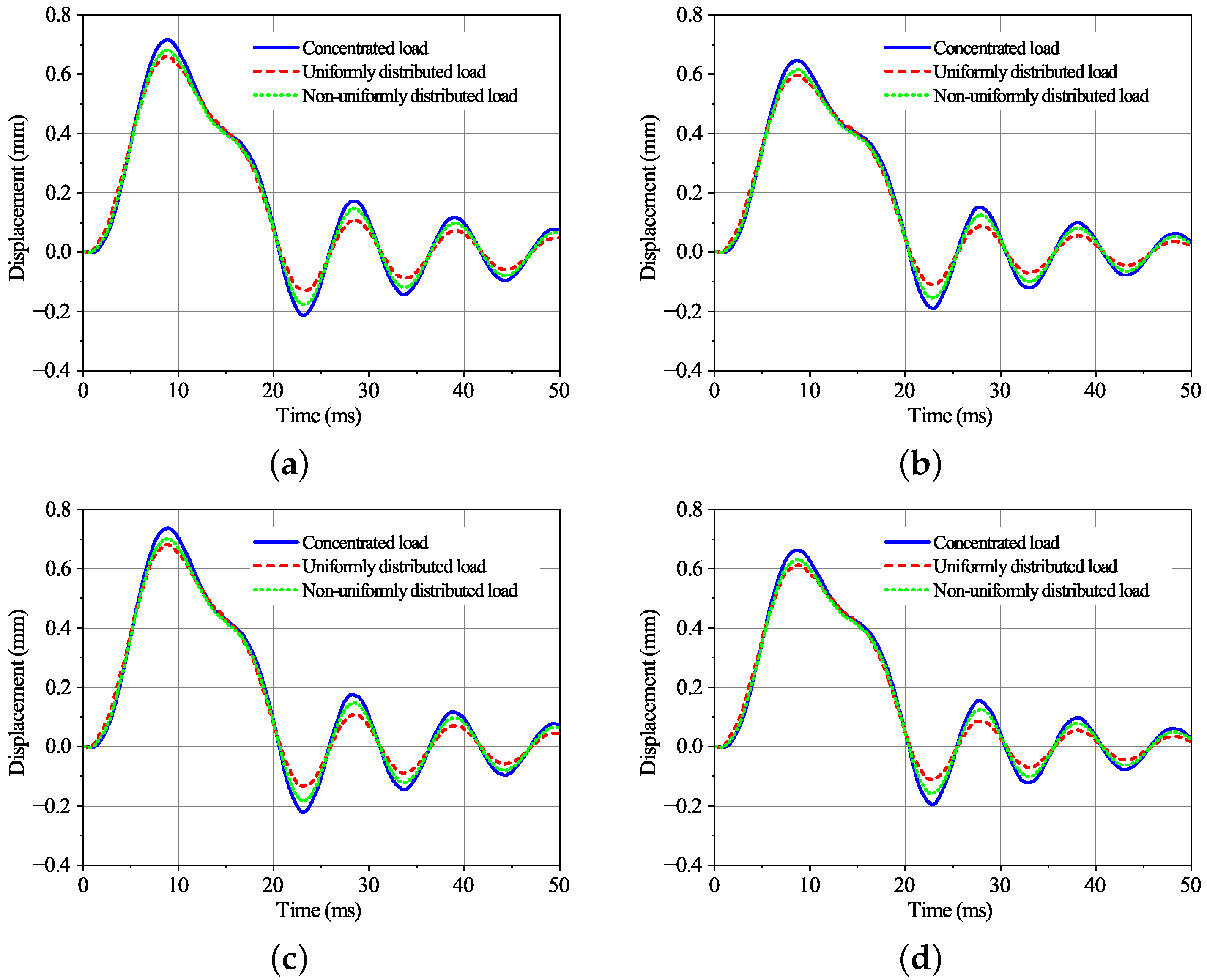
It is assumed that $v_{\mathrm{load}}=100\mathrm{m}/\mathrm{s}$, $\tilde{l}/L=0.3$, ${\lambda }_1={\lambda }_2=0.5$, $n=2$. Figure 11 compares the displacement histories of the midpoint of the beam under the three kinds of loads in different situations. It can be seen that there are apparent differences between the dynamic responses computed by the three load models in all cases. For example, in the case of power material gradient and a linear varying foundation, as Figure 11a shows, compared with the first peak displacement under the non-uniformly distributed load, that under the concentrated load is 4.82% higher, while that under the uniformly distributed load is 3.33% lower. For another example, in the case of exponential material gradient and parabolic varying foundation, the first peak displacement under the concentrated load is 4.70% higher than that under the non-uniformly distributed load, while the one under the uniformly distributed load is 3.17% lower than that. In the other two cases, as shown in Figure 11b,c, similar phenomena are also observed.

The load models also affect the calculated results of the maximum displacement $W_{\max }=max\left(\right|w(x,t)\left|\right)$ as the loads travel through the beam, as shown in Figure 12. Compared with the maximum displacement computed by the non-uniformly distributed load model, the results computed by the concentrated load model are greater, while the results calculated by the uniformly distributed load model are smaller, regardless of the travel speed. The maximum difference between the results obtained by the non-uniformly distributed load model and the concentrated load model is 5.41% in the case of the power-graded material and linearly varying foundation, as shown in Figure 12a. In the other three cases, this value is respectively 5.45%, 5.46%, and 5.39%. The maximum difference between the results obtained by the non-uniformly distributed load model and the uniformly distributed load model in the four cases are respectively 3.33%, 3.24%, 3.20%, and 3.17%. It should be pointed out that these differences increase as the ratio of the load span to the length of the beam ($\tilde{l}/L$) increases, as shown in Figure 13. For non-uniformly and uniformly distributed loads, the increase in the load span reduces the maximum displacement, which is more obvious for the uniform one. This can be concluded by comparing the downward trend of the green and red lines in Figure 13.

Although the total work of the concentrated moving load is equivalent to that of the non-uniformly distributed moving load, the concentrated load model makes the external force act on the concentrated point, which is difficult to make appear in practice, and the concentrated load will increase the local displacement, resulting in the distortion of the calculation results. In addition, the load is simplified to a uniformly distributed load, resulting in a difference between the distribution of the load and the actual load, so that the calculated displacement is less than the actual displacement, also resulting in a distortion of the calculation results. In addition, the variable local characteristics of non-uniform cross-section functionally graded beams also lead to errors in different load models. The above results indicate that, although the concentrated load model and the uniformly distributed load model are usable idealized models of realistic non-uniformly distributed loads in some situations, their errors cannot be ignored. The concentrated load model can produce values larger than the real results. The uniformly distributed load, on the contrary, produces smaller results.

5.2. Effects of the Inhomogeneous Viscoelastic Foundation

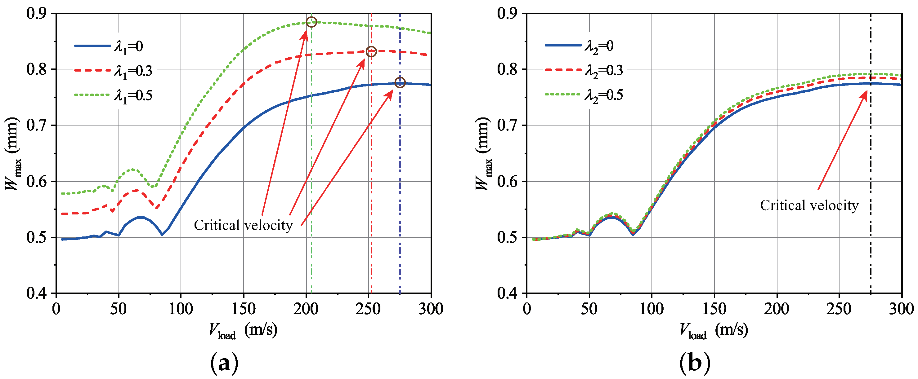
To investigate the effects of the inhomogeneous foundations on the dynamic responses of the beam, the displacement histories of the midpoint for various foundations are computed and plotted in Figure 14. The following parameters are used, including $v_{\mathrm{load}}=100\mathrm{m}/\mathrm{s}$, $\tilde{l}=0.2L$, and $n=2$. It can be seen that, compared with the dynamic responses in the homogeneous foundation case, where ${\lambda }_1={\lambda }_2=0$, those in the inhomogeneous foundation cases are higher, especially the peak values. Their oscillation periods are also longer than those of the homogeneous foundation case. The differences are more obvious in the case of linear foundations. Furthermore, the velocity of moving load also affects the maximum displacement of the beam when the magnitude is unchanged. Figure 15a indicates that the maximum displacement of the beam increases with the increase of the moving velocity initially and then decreases slowly. There exist critical velocities which result in maximum vibration amplitudes, as the circles show. A valuable discovery is that the variation of ${\lambda }_1$ results in remarkable changes in the critical velocity. On the other hand, the variation of ${\lambda }_2$ has almost no influence on the critical velocity, as shown in Figure 15b. These results indicate that the inhomogeneous foundation can significantly affect the dynamic response of beams under moving loads. The reason for the change in vibration amplitude is that the inhomogeneous foundation affects the stiffness and mode of the whole system. The influence on the critical velocity of the system is due to the fact that the critical velocity of the system is related to the wave velocity of the beam–foundation system because the occurrence of the inhomogeneous foundation reduces the wave velocity of the system and thus reduces the critical velocity.

5.3. Effects of the AFG Material

This section investigates the effects of the AFG materials on the dynamic response of the beam. In the analysis, the non-uniformly distributed load model and the parabolically varying foundation are adopted. The following parameters are used: $v_{\mathrm{load}}=100\mathrm{m}/\mathrm{s}$, $\tilde{l}=0.2L$, ${\lambda }_1={\lambda }_2=0.5$. The effects of the material gradient index n on the mid-point displacement of the beam are shown in Figure 16, considering both types of AFG materials. It shows that the AFG materials change the forced vibration response of the beam considerably. The maximum displacements of the mid-point and the value of the first peak, are reduced, compared with the case of homogeneous material (i.e., $n=0$). However, the values of the other peaks are increased. Furthermore, the vibration periods of the AFG beams are longer than those of the homogeneous beam. The variation of the maximum displacement of the whole beam as the material gradient index increases is shown in Figure 17. The maximum displacement decreases as the index increases, initially rapidly and then slowly. When $n>4$, its value is nearly unchanged as the index increases. These results indicate that the AFG materials can reduce the maximum displacement of the beam. This conclusion can be further confirmed by Figure 18, which shows the variation of the maximum displacement of the beam as the velocity of the moving load changes. Compared with the beam made of homogeneous material, i.e., $n=0$, the AFG beams made of the two components have smaller maximum displacements. The material gradient increases the overall stiffness of the system, so that the peak value of the vibration amplitude decreases, while the other peak values decrease because, under the same foundation, the material gradient reduces the amplitude of the first vibration and weakens the damping effect of the foundation. The above results inspire the idea that the FGMs can be used to optimize the dynamic response of beams under moving loads, especially to reduce the maximum displacement of the beams as the loads travel through.

6. Conclusions

This paper analyzes the dynamics of AFG beams resting on inhomogeneous viscoelastic foundations subjected to non-uniformly distributed moving loads. A consistent discrete governing equation that can tackle all the axially varying properties, including viscoelastic foundations, moving distributed loads, functionally graded materials, and cross-sections, is derived based on the Timoshenko beam theory and a Chebyshev spectral method. High-order Chebyshev expansions are employed to approximate the spatial variation of all these variable properties in a unified way and boundary conditions are imposed using a projection matrix method. Two numerical examples are given to evaluate the convergence and accuracy of the proposed method. The results, including natural frequencies and dynamic responses, are compared with those obtained by the FEM or in the literature. Good convergence and excellent accuracy are observed, demonstrating the validity of the proposed method.

The validated method is then used to investigate the effects of inhomogeneous viscoelastic foundations, AFG materials, and non-uniformly distributed moving loads on the dynamic response of beams. First, a comparison of three moving load models is carried out. They include the realistic non-uniformly distributed moving load model and two idealized equivalent models, i.e., the concentrated moving load model and the uniformly distributed load model. The results show that they are equivalent in most cases, but have some non-negligible differences in some cases. The calculated dynamic response, based on the idealized concentrated load model, including the peak displacements and the maximum displacement when moving loads travel through, will be greater than those based on the non-uniformly distributed moving load model. Conversely, the results obtained by the uniformly distributed load model will be smaller. Second, the effects of inhomogeneous viscoelastic foundations are studied. It can be found that the varying properties of the foundations can alter the maximum displacement and critical speed of beams under moving loads significantly. Finally, the dynamic responses of different AFG beams are compared with those of corresponding homogeneous beams. The results demonstrate that the AFG materials apparently affect vibration amplitudes and periods.

The proposed numerical method and computational model are available for beams with arbitrary axially varying properties, including AFG materials, inhomogeneous viscoelastic foundations, non-uniform cross-sections, and that are non-uniformly distributed, thus having a wide scope of application. The application of functionally graded materials in high-speed moving loads, such as electromagnetic rail guns and rocket sleds, will make it possible to reduce structural vibration and improve structural stability, thus further improving the limiting speed of the structure. The results of the analysis in this paper provide important support for the design and application of functionally graded materials in complex engineering structures.

References

- Lamprea-Pineda, A.C.; Connolly, D.P.; Hussein, M.F.M. Beams on elastic foundations—A review of railway applications and solutions. Transp. Geotech. 2022, 33, 100696. [Google Scholar] [CrossRef]
- Plaut, R.H.; Dillard, D.A. Rigid wheel/roller on infinite beam or plate attached to winkler, pasternak, or elastomeric foundation. Int. J. Solids Struct. 2023, 262–263, 112001. [Google Scholar] [CrossRef]
- Quzizi, A.; Abdoun, F.; Azrar, L. Nonlinear dynamics of beams on nonlinear fractional viscoelastic foundation subjected to moving load with variable speed. J. Sound Vib. 2022, 523, 116730. [Google Scholar]
- Fallah, A.; Aghdam, M.M. Physics-informed neural network for bending and free vibration analysis of three-dimensional functionally graded porous beam resting on elastic foundation. Eng. Comput. 2023. [Google Scholar] [CrossRef]
- Ermis, M.; Kutlu, A.; Omurtag, M.H. Free vibration of axially FG curved beam on orthotropic Pasternak foundation via mixed FEM. J. Braz. Soc. Mech. Sci. Eng. 2022, 44, 597. [Google Scholar] [CrossRef]
- Vu, A.N.T.; Le, N.A.T.; Nguyen, D.K. Dynamic behaviour of bidirectional functionally graded sandwich beams under a moving mass with partial foundation supporting effect. Acta Mech. 2021, 232, 2853–2875. [Google Scholar] [CrossRef]
- Jena, S.K.; Chakraverty, S.; Malikan, M. Application of shifted Chebyshev polynomial-based Rayleigh–Ritz method and Navier’s technique for vibration analysis of a functionally graded porous beam embedded in Kerr foundation. Eng. Comput. 2021, 37, 3569–3589. [Google Scholar] [CrossRef]
- Nguyen, N.D.; Vo, T.P.; Nguyen, T.K. An improved shear deformable theory for bending and buckling response of thin-walled FG sandwich I-beams resting on the elastic foundation. Compos. Struct. 2020, 254, 112823. [Google Scholar] [CrossRef]
- Calim, F.F. Free and forced vibration analysis of axially functionally graded Timoshenko beams on two-parameter viscoelastic foundation. Compos. Part B Eng. 2016, 103, 98–112. [Google Scholar] [CrossRef]
- Yas, M.H. Free vibrations and buckling analysis of carbon nanotube-reinforced composite Timoshenko beams on elastic foundation. Int. J. Press. Vessel. Pip. 2012, 98, 119–128. [Google Scholar] [CrossRef]
- Li, Z.; Xu, Y.; Huang, D. Analytical solution for vibration of functionally graded beams with variable cross-sections resting on Pasternak elastic foundations. Int. J. Mech. Sci. 2021, 191, 106084. [Google Scholar] [CrossRef]
- Nayak, D.K.; Dubey, A.; Nayak, C.R. Free and forced vibration of coupled beam systems resting on variable viscoelastic foundations. Int. J. Struct. Stab. Dyn. 2020, 42, 130. [Google Scholar]
- Nayak, D.K.; Dubey, A.; Nayak, C.R.; Dash, P.R. Stability analysis of an exponentially tapered, pre-twisted asymmetric sandwich beam on a variable Pasternak foundation with viscoelastic supports under temperature gradient. J. Braz. Soc. Mech. Sci. Eng. 2020, 42, 130. [Google Scholar] [CrossRef]
- Coskun, S.B.; Ozturk, B. Elastic Stability Analysis of Euler Columns Using Analytical Approximate Techniques. Adv. Comput. Stab. Anal. 2012, 6, 115–132. [Google Scholar]
- Kumar, S. Dynamic behaviour of axially functionally graded beam resting on variable elastic foundation. Arch. Mech. Eng. 2020, 67, 451–470. [Google Scholar]
- Jorge, P.C.; Simoes, F.M.F.; Costa, A.P.D. Dynamics of beams on non-uniform nonlinear foundations subjected to moving loads. Comput. Struct. 2015, 148, 26–34. [Google Scholar] [CrossRef]
- Zarfam, R.; Khaloo, A.R. Vibration control of beams on elastic foundation under a moving vehicle and random lateral excitations. J. Sound Vib. 2012, 331, 1217–1232. [Google Scholar] [CrossRef]
- Esen, I. Dynamic response of a functionally graded Timoshenko beam on two-parameter elastic foundations due to a variable velocity moving mass. Int. J. Mech. Sci. 2019, 153–154, 21–35. [Google Scholar] [CrossRef]
- Li, B.; Wang, S.; Wu, X.; Wang, B. Dynamic response of continuous beams with discrete viscoelastic supports under sinusoidal loading. Int. J. Mech. Sci. 2014, 86, 76–82. [Google Scholar] [CrossRef]
- Calim, F.F. Dynamic analysis of beams on viscoelastic foundation. Eur. J. Mech. A Solids 2009, 28, 469–476. [Google Scholar] [CrossRef]
- Younesian, D.; Kargarnovin, M.H.; Thompson, D.J.; Jones, C.J.C. Parametrically Excited Vibration of a Timoshenko Beam on Random Viscoelastic Foundation jected to a Harmonic Moving Load. Nonlinear Dyn. 2006, 45, 75–93. [Google Scholar] [CrossRef]
- Kargarnovin, M.H.; Younesian, D. Dynamics of Timoshenko beams on Pasternak foundation under moving load. Mech. Res. Commun. 2004, 31, 713–723. [Google Scholar] [CrossRef]
- Wang, Y.; Zhou, A.; Fu, T.; Zhang, W. Transient response of a sandwich beam with functionally graded porous core traversed by a non-uniformly distributed moving mass. Int. J. Mech. Mater. Des. 2020, 16, 519–540. [Google Scholar] [CrossRef]
- Zhang, Y. Steady state response of an infinite beam on a viscoelastic foundation with moving distributed mass and load. Sci. China Phys. Mech. Astron. 2020, 63, 284611. [Google Scholar] [CrossRef]
- Nguyen, D.K.; Vu, A.N.T.; Le, N.A.T.; Pham, V.N. Dynamic Behavior of a Bidirectional Functionally Graded Sandwich Beam under Nonuniform Motion of a Moving Load. Shock Vib. 2020, 2020, 8854076. [Google Scholar] [CrossRef]
- Wang, Y.; Zhu, X.; Lou, Z. Dynamic response of beams under moving loads with finite deformation. Nonlinear Dyn. 2019, 98, 167–184. [Google Scholar] [CrossRef]
- Assie, A.; Akbaş, Ş.D.; Bashiri, A.H.; Abdelrahman, A.A.; Eltaher, M.A. Vibration response of perforated thick beam under moving load. Shock Vib. 2021, 136, 283. [Google Scholar]
- Yagci, B.; Filiz, S.; Romero, L.; Ozdoganlar, O.B. A spectral-Tchebychev technique for solving linear and nonlinear beam equations. J. Sound Vib. 2020, 321, 375–404. [Google Scholar] [CrossRef]
- Zhao, Y.; Huang, Y.; Guo, M. A novel approach for free vibration of axially functionally graded beams with non-uniform cross-section based on Chebyshev polynomials theory. Compos. Struct. 2017, 168, 277–284. [Google Scholar] [CrossRef]
- Mashat, D.S.; Carrera, E.; Zenkour, A.M.; Khateeb, S.A.A.; Filippi, M. Free vibration of FGM layered beams by various theories and finite elements. Compos. Part B Eng. 2014, 59, 269–278. [Google Scholar] [CrossRef]
- Assaee, H.; Hasani, H. Forced vibration analysis of composite cylindrical shells using spline finite strip method. Thin-Walled Struct. 2015, 97, 207–214. [Google Scholar] [CrossRef]
- Pham, V.V.; Nguyen, V.C.; Hadji, L.; Mohamed-Ouejdi, B.; Ömer, C. A comprehensive analysis of in-plane functionally graded plates using improved first-order mixed finite element model. Mech. Based Des. Struct. Mach. 2023, 2245876. [Google Scholar] [CrossRef]
- Wang, T.M.; Stephens, J.E. Natural frequencies of Timoshenko beams on Pasternak foundations. J. Sound Vib. 1977, 51, 149–155. [Google Scholar] [CrossRef]
- Hou, Y.C.; Tseng, C.H.; Ling, S.F. A new high-order non-uniform timoshenko beam finite element on variable twoparameter foundations for vibration analysis. J. Sound Vib. 1996, 191, 91–106. [Google Scholar] [CrossRef]