
Concealed Conduit Routing in Building Slabs

Department of Computer Science and Engineering, National Taiwan Ocean University, No. 2, Peining Road, Keelung 202301, Taiwan
*
Author to whom correspondence should be addressed.
Appl. Sci. 2023, 13(19), 10847; https://doi.org/10.3390/app131910847
Submission received: 31 August 2023
/
Revised: 25 September 2023
/
Accepted: 26 September 2023
/
Published: 29 September 2023
(This article belongs to the Topic Innovation of Applied System)
Abstract
:Featured Application
The proposed piping algorithm and data structures can benefit the construction and manufacturing industries.
Abstract
Concealed pipes are vital facilities for transporting water, air, electricity, and natural gas in modern buildings. These pipes are constructed inside slabs of buildings, and thus conventional piping algorithms, dedicated to arranging exposed pipes in open spaces or on object surfaces, are not suitable for laying out their paths. In this article, an innovative method is presented for designing the concealed conduits of modern buildings. In the proposed piping procedure, the target building is regarded as a framework composed of beams, columns, and slabs. These substructures are encoded in a weighted graph, which serves as the top-level representation of the workspace. Then, these substructures are split into voxels and constitute the bottom-level representation of the workspace. Each concealed pipe is constructed by using a two-stage piping scheme to comply with the representation of the workspace. In the first stage, the slabs containing the terminals of the pipe are located in the top-level representation, and the shortest path connecting these slabs is calculated using Dijkstra’s algorithm. In the second stage, a feasible space is generated by collecting selective voxels in these slabs first. Then, the pipe path is routed inside the feasible space by a shortest-path-finding computation. Next, the pipe surface is generated and represented by using triangle meshes. Finally, the bottom-level representation is modified and the routing process is repeated to lay out the remaining concealed pipes. The experimental results show that the proposed piping procedure efficiently arranges concealed pipes inside buildings of various topologies and internal layouts. As it benefits from the two-level representation and the two-stage routing method, the piping process consumes reasonable computational costs. The paths of the resultant pipes are optimized, and their positions meet the geometrical constraints and safety regulations.
1. Introduction
Pipe systems are widely used in vehicles, engines, factories, and refineries to transport fuels, water, air, and raw materials. They are essential components in the manufacturing, chemical, and transportation industries. Many efficient algorithms have been proposed for routing them since the 1970s [1,2]. Since pipes are utilized in various applications [3,4,5,6], the paradigms, domain representation methods, and limitations of these published algorithms are different. However, they share a common aspect: The target pipes are exposed conduits. That is, they aim to lay out pipes in open spaces or on the surfaces of objects, and the resultant pipes are visible and accessible to the users.
In modern buildings, there are hoses, conduits, and wire harnesses inside the walls, floors, and ceilings. These pipes are invisible and inaccessible to us but we rely on them to deliver ventilation air, tap water, electrical power, digital signals, and natural gas such that decent living and working conditions can be maintained. In construction industries, these pipes are included in the Mechanical Electronic and Plumbing (MEP) systems and must be carefully planned prior to the construction of the buildings [6,7,8].
Figure 1 reveals the major difference between exposed conduit systems (left part) and concealed conduit systems (right part). The exposed conduits are routed in open spaces or on the surfaces of machinery. They may penetrate the walls to connect terminals residing in different rooms, but their paths do not reside below the surfaces of the walls and the machinery. On the other hand, the concealed pipes are built inside the walls, floors, and ceilings of the building. They wander in the walls, floors, and ceilings to connect terminals. Their paths are laid out within the slabs of the building.
Solely based on the functionality of transportation, concealed conduits can be replaced with exposed ones. However, concealed conduits possess at least the following advantages over exposed pipes: (1) They do not occupy valuable living space; (2) they do not hinder the operations of machinery and the movement of humans; (3) they do not need supporting racks; (4) they are resilient to intentional or unintentional collisions; (5) and for the sake of aesthetics, they do not produce unpleasant visual effects. Therefore, concealed conduits are widely installed in modern buildings, and routing them is an important issue in building design and construction.
The complexity and costs of a pipe-routing process are significantly influenced by the characteristics of the workspace [1]. Exposed pipes are laid in open spaces or on the surfaces of machinery [2,3,4,5]. Their workspaces are extensible and more flexible. On the other hand, concealed conduits are buried inside the walls, floors, ceilings, columns, and beams of buildings. Their workspaces are confined within these substructures only and are impossible to extend. Furthermore, staircases, windows, and doors in the buildings significantly reduce the usable portions of the workspace and increase the geometric complexity of the workspaces. To make matters worse, concealed pipes should be buried below the surfaces of these substructures at a certain distance such that they will not be damaged when the surfaces are hammered, decorated, or tiled. Hence, the workspace of a concealed conduit system is much thinner and more limited than expected. The examples shown in Figure 1 reveal the characteristics of the working domains of concealed pipes.
In addition to overcoming the above challenges, the transportation functionalities, construction costs, and safety regulations must be also taken into consideration when routing concealed conduits. These requirements make laying out concealed conduits more difficult. Conventional piping algorithms are not suitable for arranging concealed conduits. Specialized routing methods and new workspace representations have to be developed to fulfill the piping task.
1.1. Methodology Overview
In this article, we propose a piping algorithm for designing concealed conduits. To conquer the aforementioned challenges, we first invent an innovative representation method to encode the workspace. Then we design a two-stage routing algorithm to compute the pipe paths. As a result, the proposed method achieves the following goals: (1) The resultant pipes are confined inside the walls, floors, and ceilings and are at a safe distance from the open space; (2) the length and number of bends of the resultant pipes are optimized; (3) the functionalities and safety regulations of the resultant pipes are satisfied; and (4) the computations are efficiently carried out without performing exhaustive search in the workspace.
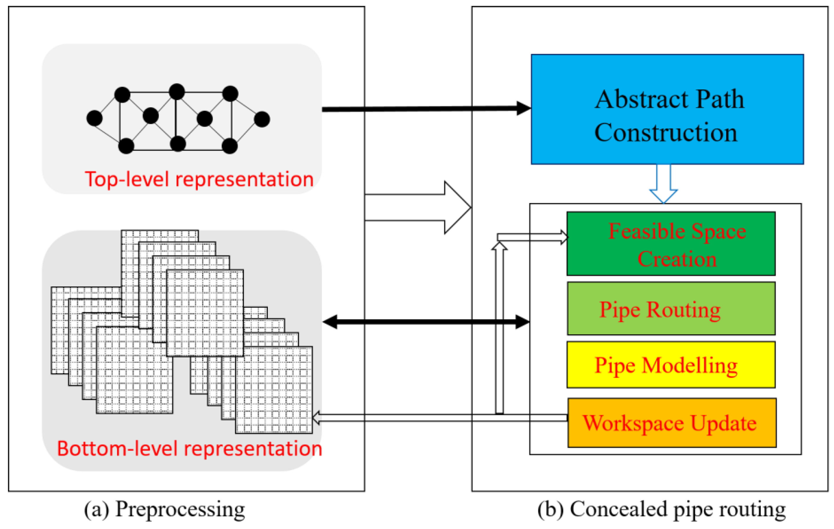
The proposed piping method is composed of two major tasks, the preprocessing and the pipe routing computations, as shown in Figure 2. The preprocessing builds a hierarchical representation of the workspace. The walls, ceiling, and floors of the target building are regarded as slabs. By representing the slabs as vertices and creating edges between them, the working environment (the target building) is converted into a weighted graph, which serves as the top level of the hierarchical representation. Then, each individual slab is decomposed into voxels and transformed into a 3D image. In the following step, the voxels of the slabs are labeled according to their positions and usability. For example, the voxels, occupied by windows, doors, and other openings, are marked as obstacle voxels, and the voxels within a predefined distance from the slab surfaces are labeled as infeasible voxels. As the labeling ends, the bottom level of the hierarchical representation is generated, as shown in Figure 2a.
The routing computation is comprised of two stages, as shown in Figure 2b. In the first stage, the proposed algorithm calculates an abstract path in the weighted graph for each pipe. Then, the pipes are routed one by one in the following computations. Before arranging a pipe, the proposed piping method creates a feasible space by using the abstract path of this pipe and the relevant slabs stored in the bottom-level representation. Next, the pipe path is calculated in the feasible space. Then, the geometric model of the pipe is generated. In the final step, the workspace is updated to reflect the existence of the pipe and the routing computations are repeated for the next pipe.
1.2. Related Work
Most piping methods treat pipe design as shortest-path-finding problems, as revealed by the investigation of [1]. In Refs. [3,6], the researchers proposed building a graph structure in the workspace. Then pipes are routed in this graph by using shortest-path-searching methods like Dijkstra’s algorithm [9] and the A* method. These two research studies adopted a widely used piping strategy, which encodes the workspace as a graph and finds the pipe paths by using A* or Dijkstra’s algorithm.
However, minimizing the costs of multiple pipes simultaneously is an NP-hard problem [1]. Using deterministic algorithms to optimize pipe routing is impractical. In Ref. [10], Qu et al. proposed routing pipes using ant colony optimization (ACO) methods. They employed swarms of artificial ants to search pipe paths and utilized pheromones to guide the ants such that good pipe paths were gradually constructed. In Ref. [11], a genetic algorithm was proposed by Ito to schedule and calculate pipes. In the method, the positions and directions of pipes are encoded in chromosomes and are revised by using cross-over, mutation, and duplication operators in the hope of generating optimal pipe routes. The domain knowledge, expertise, and experiences of engineers are valuable resources for solving piping problems. In Ref. [12], scientists designed expert systems, incorporating computational power and memory capacities of computers and human wisdom, to design optimal pipe routes. The above research utilizes artificial intelligence techniques to find optimal answers in the solution space such that an exhaustive search can be avoided.
Besides being economical, a pipe must also meet safety regulations such that potential hazards are avoided, and the operational and maintenance costs can be minimized. Ueng et al. proposed creating a distance field in the workspace to eliminate infeasible space before routing pipes [4]. Consequently, the resultant pipes possess minimum lengths and meet all safety regulations. In the work of [13], an ACO path-finding procedure is proposed to route a water distribution network. The researchers proposed utilizing geometrical information systems to adapt critical path analysis such that unwanted paths are removed and optimal water pipes are searched. In the studies of [10,11], the researchers rely on a fitness function or a cost function to direct the path-finding process. Hence, the costs of violating safety regulations are high and the resultant pipes will be routed away from hazards. This strategy prevents violations of safety regulations by penalizing the improper paths. However, it cannot eliminate the possibility of violating constraints, and the safe gaps between the pipes and the hazards are not guaranteed.
Pipe-routing algorithms have been widely used for designing MEP systems of buildings. In [6], Choi et al. devised a modified A* method for creating MEP paths. In their method, the workspace is imported from a Building Information Modeling (BIM) [7] system first. Then, nodes, sub-MEP, and main-MEP systems are created in the building’s space. In the following computation, a modified A* algorithm is employed to find the shortest paths for the MEP systems. Zhang et al. proposed a routing algorithm in [14] for the design of drainage systems of panelized residential buildings. The researchers employed a modified A* algorithm to arrange the paths of the drainage systems. Since the drainage and vent pipes must be cut at the edges of panels, they also developed an integer programming approach for optimizing the pipe-cutting process. They embedded their piping program into commercial software and demonstrated a successful experiment in a two-story townhouse of five identical units. As modularization and prefabrication are widely used for building construction, Samasinghe et al. proposed an optimization method for modular prefabrication of MEB systems [15]. Their approach combines fuzzy logic, a dependency structure matrix, and hierarchical clustering techniques. Their goal is to minimize installation costs by identifying the optimum number of modules and the best division points of the MEB systems. The goals of these studies are similar to ours. The resultant pipes are part of MEB systems. However, the workspace of our method is different from theirs. Our routing environment is confined within the slabs of buildings.
Electrical system design is vital for buildings and communities. Farooq et al. presented studies on the supportive roles of BIM tools in the design, analysis, planning, and construction of electrical trade systems [16]. They found that the combination of BIM and GIS is useful for smart electrical grid construction. Managing the construction of MEB systems is as important as the design work. In the paper of [17], Teo et al. expanded the functionalities of BIM systems and incorporated construction management techniques for building MEB systems. Their 3D MEB design system offers a visualization function such that the target MEB system can be visually explored before the installation. Their system reduces manual work and resolves conflicts by developing better workflows and management strategies. As a result, the productivity, accuracy, and efficiency of the construction works are increased while the building expense is reduced. These investigations verify that the BIM systems of buildings have become the de facto digital representation methods in modern construction industries, and the geometrical information of the resultant pipes of the MEB systems should be integrated into BIM systems. Piping is no longer a standalone process.
The representation of the workspace influences the efficiency of the routing process. In most published studies, the workspaces and the pipes were represented by a single layer of structures. In the work of [18], Yue et al. proposed a hierarchical layout of the subsea production control system in the 3D undersea working environment. In their approach, they used a multi-layer star-tree structure to create the layout of the control network. To find the optimal layout, they combined the construction costs of the control center, distribution units, control modules, and umbilical and fly lines to form an objective function. Then, they applied constraints upon the design such that the connection, terrain, position, and pipe route requirements could be met. Finally, they utilized A* and swarm-intelligence algorithms to solve the system and generate the resultant production control system. Their problem domain representation method is hierarchical. However, the representation is an abstract structure, a multi-layer star tree in the 3D undersea space. On the other hand, our workspace encoding scheme uses both an abstract graph and a set of solid 3D images (the slabs). Hence, ours is more suitable for the routing process inside the walls, floors, and ceilings of buildings.
The piping algorithms invented by these related research studies focused on routing exposed conduits in open spaces or on object surfaces. Their workspace representation schemes are not suitable for encoding the slabs of a building. Their path-finding methods cannot explore the internals of the slabs. Employing their piping algorithms to arrange concealed conduits would result in unqualified pipes or violations of safety regulations and geometric constraints. Thus, in this research, we propose a new piping algorithm dedicated to laying out concealed conduits in modern buildings.
The rest of this article is organized as follows: Our workspace-encoding strategy and path-finding scheme are described in Section 2. Test results are presented and explained in Section 3. The discussion, potential applications, and future work are contained in Section 4. This article ends with the conclusion part in Section 5.
2. Materials and Methods
The proposed piping method is composed of two computations, the preprocessing and the pipe routing computation. The first computation generates a digital representation of the workspace while the second one constructs the pipes. The digital representation encodes essential information about the workspace and ensures the efficiency of the path-finding computation. In turn, its contents will be altered by the routing process at the run-time. In this section, we first present the workspace encoding scheme. Then, we describe the path-finding procedure. The interdependence between these two computations will also be explained.
2.1. Workspace Representation
The framework of a modern building is composed of columns, beams, walls, floors, and ceilings as shown in Figure 3. The walls, ceilings, and floors are slabs, which are parallel to the xy-, yz-, and zx-planes of the world coordinate system. These slabs constitute the workspace for pipe-routing in this research. On the other hand, the columns and beams are regarded as connectors, and their spaces are shared by the slabs. In the proposed piping method, we design a hierarchical representation to encode the building such that the workspace can be fully explored and easily updated at the run time. Consequently, high-quality pipe paths can be produced, and exhaustive searching can be prevented. The encoding schemes are presented in the following sections.
2.1.1. The Top-level Representation
The top level of the hierarchical representation is a weighted graph G, which contains a vertex set V and an edge set E, i.e., G = {V, E}. We regard the slabs of the target building as vertices and keep them in V. Then, we check the adjacency relations among the slabs to create E. If two slabs are adjacent by sharing a beam or a column, then an edge is produced between them. This edge is associated with a positive weight.
Assuming that these two slabs are S1 and S2, their centers are C1 and C2, and the edge connecting S1 and S2 is E12, then the weight of E12 is decided as follows:
- If S1 and S2 are coplanar, the edge weight is equal to the Manhattan distance between C1 and C2.
- Otherwise, the edge weight is set to 1.5 times the Manhattan distance between C1 and C2.
The weight of E12 approximates the shortest path length from C1 to C2. If S1 and S2 are coplanar, a path from C1 to C2 contains no bend, and thus the weight of E12 is set to the Manhattan distance between C1 and C2. On the other hand, if S1 and S2 are not coplanar, this path must make a 90-degree turn inside a beam or a column. In this situation, we increase the edge weight to reflect the existence of the bend and give a penalty to the path. By adopting these two principles, we hope that the pipe path will make fewer turns and contain longer straight segments.
Figure 4 shows an example of the top-level representation. The left part contains a simple building composed of six slabs. The top-level representation of the simple building is shown in the right part. There are six vertices in the graph. Each vertex has four neighbors since each slab is adjacent to four slabs in this case. All the slabs are not coplanar. Thus, the edge weights are equal to 1.5 times the Manhattan distances of the centers of the neighboring slabs.
- Usage and limitation of the top-level representation
Graph G stores the connectivity and distances between the slabs. It also implicitly records the sizes of the slabs and their co-planarity relations. If we compute the shortest path from slab Sa to slab Sb, this path will prefer small and coplanar slabs because of the algorithm employed for computing the path and the way in which we define the edge weights. Graph G can be used to produce the target pipes only if all the terminals reside at the slab centers. However, the terminals of the target pipes could be at any position in the slabs. The pipes created upon G cannot correctly connect them. Secondly, there are openings in the slabs, the target pipes must bypass these obstacles. Thirdly, the target pipes must be buried inside the slabs at a safe distance from the surfaces of the slabs. Graph G does not record depth information about the workspace. These issues imply that the information stored in G is not enough for routing the target pipes, and hence a finer representation of the workspace is needed for the pipe-routing process.
2.1.2. The Bottom-level Representation
After creating the weight graph G, we split each slab into voxels by using a regular grid. The width of a voxel is decided by the users (for example 1 cm). Henceforth, the slabs become 3D images of voxels and the bottom-level representation of the building is initialized. An example is shown in Figure 5. In this example, each slab is decomposed into a layer of voxels. However, in a practical case, a slab will consist of more than ten layers of voxels.
- Obstacle voxel labelling
Since there are windows, doors, and stair openings inside the slabs, the 3D images have to be further processed to exclude these obstacles. First, the voxels that belong to doors, windows, and other openings are identified and given a special tag. Hereafter, they are inferred as obstacle voxels.
- Distance field computation
Then, a distance field is established in the slab by using the Chamfer transformation [13]. The algorithm can be briefly formulated as follows:
- The voxels adjacent to the open space or the obstacle voxels are identified. They form the boundaries of the distance field.
- The distance values in these boundary voxels are set to one-half of the voxel size.
- Then, the distance field is expanded by using a multiple-sweeping method until the distances of all the ordinary voxels have been computed.
The detailed steps of the sweeping can be found in [19]. We omit it here. Chamfer transform is known to be fast but inaccurate. In this study, the accuracy of the distance field is not crucial. If higher precision computations are required in the distance field computation, the methods presented in [20,21] are good choices.
- Peeling the slabs
After the distance field is calculated, the minimum distance from each non-obstacle voxel toward the workspace boundaries is known. Since the surface of each pipe must be at a safe distance from the open space, the voxels within this safe distance are found and excluded from the workspace. They are regarded as infeasible voxels. They are not used for routing pipe paths, but they can be used to construct pipe surfaces. Next, the remaining voxels are labeled as ordinary voxels and will participate in the following routing procedure.
- Bottom-level representation updating
When a pipe is created, the voxels penetrated by it cannot be used to fabricate other pipes and must be deleted from the workspace. Consequently, the distance field and voxel labels in each slab have to be modified at the run-time. The bottom-level representation is hence a dynamic data structure. Its contents (voxel labels and distance values) are constantly changed as the pipe-routing process progresses.
2.2. Pipe Path Routing
Once the hierarchical representation of the workspace has been created, the pipe-routing process starts. The routing process is composed of two stages. The abstract paths of the pipes are computed in the first stage while the real pipe paths are routed in the second stage. The key modules of our pipe routing method are presented in this section, including abstract path generation, pipe scheduling, feasible space creation, and pipe creation steps.
2.2.1. Abstract Pipe Path Calculation
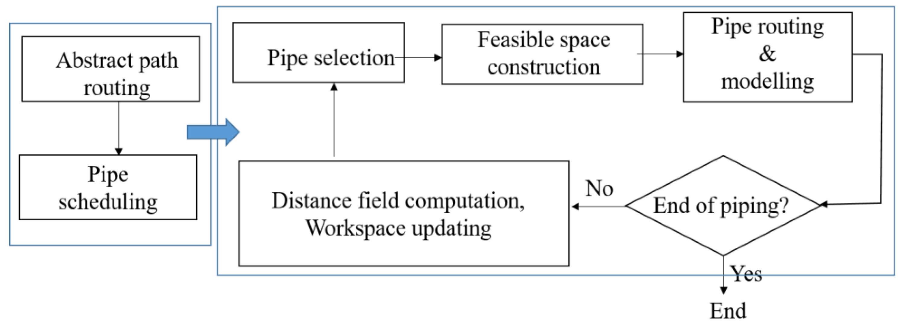
The flowchart of the routing process is shown in Figure 6. The routing process starts with the abstract path routing. The abstract path of a pipe is the shortest path generated in the top-level representation. It is utilized to schedule the pipe and generate a subspace to lay out the real pipe path. The abstract path is produced by the following steps:
- Locate the vertices (slabs) in G, which contain the terminals of this pipe.
- Generate a shortest path to connect these vertices using Dijkstra’s algorithm.
- Duplicate the slabs containing multiple terminals: If a slab contains k terminals (k ≥ 2), the associated vertex is duplicated k times in the shortest path.
- Compute the path length by accumulating the weights of the edges in the shortest path. If the two ends of an edge are the same, its weight is set to one-half of the width of the slab. (We assume that the slab width > the slab height.)
- Output the length and vertices of this shortest path.
The abstract path is a sketch of the real pipe path. Its vertices represent the slabs that would be penetrated by the pipe, and its length is an estimation of the length of the real pipe path. These two pieces of data are used in the incoming computations.
2.2.2. Pipe Ordering
As revealed in Figure 6, the pipe scheduling is performed after all the abstract paths have been constructed. Since a building usually possesses multiple concealed pipes, pipe scheduling is a necessary job in the piping process. A good schedule can greatly reduce the total costs of the resultant pipes. Unfortunately, the optimum scheduling problem of pipe routing is NP-hard [1], and pursuing the best schedule is impractical.
In this research, we order the pipes based on a principle published in [1]. This principle suggests that long and thick pipes should be routed first such that the utilization of the workspace will be higher, and the quality of the final pipe paths could be better. This principle was widely used in pipe-routing computations and has been proven to be effective [3,4,5,6]. Nonetheless, it is logically contradictory for this research since the actual lengths of the concealed pipes are unknown before the routing process starts. To resolve this conflict, we sort the pipes according to the lengths of their abstract paths.
The rationale supporting this approach can be explained as follows: The abstract path of an individual concealed pipe records the slabs that will be penetrated by this pipe. The sizes of these slabs and the coplanar relationships between these slabs are reflected by the length of the abstract path. If the length of the abstract path is longer, then at least one of the following conditions is true: (1) This pipe would go through larger slabs (longer length), (2) the pipe would penetrate slabs that are not coplanar (more bends), (3) the pipe would cover more slabs (longer length), or (4) the pipe has many terminals (more branches). Based on these conditions, this pipe is likely to be long and consume more spatial resources. It should be given a higher priority over other pipes.
Other widely used criteria for ordering pipes include the sizes, functionalities, and safety regulations of the pipes. Large pipes need more space. It is difficult to arrange optimal paths for them if the available spaces are occupied by other pipes. Therefore, they should be built earlier. However, concealed conduits are buried inside slabs. Their sizes will be approximately equal. Pipe lengths are more important for scheduling pipes. It is not uncommon that some pipes are more essential than others, for example, the electricity harnesses in a manufacturing factory. In other cases, safety regulations are the key factors, for example, natural gas pipes in a building with cooking or heating facilities. Under these conditions, the functionalities and safety regulations of pipes play key roles in the pipe scheduling process. However, in this research, we regard merely the pipe lengths as the only factor when scheduling the pipes. Other considerations would be included in the future work.
2.2.3. Feasible Space Creation
Once the pipes are sorted, they are to be routed one by one. When routing a pipe, we can optimize its costs by searching the entire workspace and selecting optimal positions to shorten its path and reduce the number of bends. However, this will lead to slow computation and unsafe pipe paths since we have to perform an exhaustive search in the workspace but do not take safety regulations into consideration.
To overcome these problems, the proposed piping method establishes a feasible space in the bottom-level representation before routing the target pipe. The feasible space covers only a small portion of the workspace, and all its voxels are collision-free and satisfy the safety regulations. Hence, the computation of path-finding is sped up, and the resultant pipe path meets the geometrical constraints and safety regulations.
- Usage of the distance field
To establish the feasible space, we retrieve the slabs of the abstract path of this pipe first. These slabs form a subspace, which can be used to lay out the pipe, but we refine it further to reduce the scope of this subspace and enforce the safety regulations and geometrical constraints upon its voxels. To do so, we scan the ordinary voxels of these slabs and collect those ordinary voxels whose distance values d(i, j, k) meet the following conditions:
where (i, j, k) denotes the indices of an individual voxel, r is the radius of the pipe, and ε1 and ε2 are user-defined parameters for controlling the spaces between the voxel and the obstacles. The collected voxels form a smaller subspace. This smaller subspace is separate from all obstacles and potential hazards by at least r + ε1 units. Its width is limited by r + ε2 units. As a result, the subspace is safe for tracing the pipe path while its scope is much smaller than the entire workspace.
- Connectivity of the terminals and safety gaps
This subspace cannot be used to route the pipe unless it contains all the terminals of the pipe. To ensure that, we examine all the terminals of the pipe and identify those who are outside this subspace. If an outsider is found, a breath-first search (bfs) [9] is triggered from that terminal and is expanded outwards until reaching the current subspace. Then, those ordinary voxels visited by the bfs are included in this subspace. Once all the terminals are inside this subspace, the creation of the feasible space is completed.
The routing of the pipe will be carried out within the feasible space. Since the voxels of the feasible space are screened by Equation (1), the searching space is greatly reduced. Furthermore, by adjusting ε1, we can create safe gaps between the feasible space and the obstacles or potential hazards. Thus, the resultant pipe path will not violate any safety regulations.
2.2.4. Pipe Path Computation
The pipe path is calculated utilizing Dijkstra’s algorithm. To do so, the proposed method treats the feasible space as a graph. Its voxels become vertices and the connectivity relations of its voxels are regarded as edges. Since this graph is created by using the voxels of the feasible space, the edges are parallel to x-, y-, or z-axes, and thus the resultant pipe path will be composed of straight lines or 90-degree bends.
- Branch scheduling
If the pipe consists of multiple branches, the proposed piping method constructs these branches one after another. At first, we compute the Manhattan distance between each pair of the terminals, and the two terminals generating the longest Manhattan distance are designated as the source and the destination. Then, a shortest path is created to connect them by using Dijkstra’s algorithm. The resultant path is the initial skeleton of the pipe. In the following step, one of the unconnected terminals is randomly selected and treated as the source, and the shortest path from this unconnected terminal to the current skeleton is computed. Once constructed, the new branch is included in the skeleton, and the above calculation is repeated to generate the remaining branches. Once all the terminals are connected, the routing process of the pipe is finished.
- Cost function of path-finding
Dijkstra’s algorithm may produce many bends and elbows in the resultant pipe path since the feasible space is built upon a regular grid. To reduce the number of bends in the pipe path, we employ a cost function C(-) to control the forward directions in the pipe path. Assuming that the current position of the routing is at voxel vi and the cost of the pipe is C(vi), then the cost for selecting the neighboring voxel vi+1 as the next position is computed by the following formula:
where v0 and v1 are the first 2 voxels in the pipe path, C(vi+1) is the new cost, and p(vi, vi+1) is the incremental value to the current cost. The incremental value is decided by the direction of the pipe path. If the pipe path marches straightforwardly, the incremental value is 1. Otherwise, the incremental value is 1 + ω, where ω a positive number, which is used to penalize the bend caused by the new voxel vi+1. In this research, ω is set to 9 to benefit straight pipe paths.
2.2.5. Pipe Surface Generation and Workspace Update
The resultant pipe path is merely the skeleton of the pipe. We have to construct a geometrical representation for the pipe. At first, we create consecutive cylinders with a radius r along the pipe path. Then we connect these cylinders to form the surface of the pipe. In the next step, the surface is discretized into a triangle mesh and kept in a disk file.
Before routing the next pipe, we modify the workspace to reflect the existence of the pipe. First, we search for the voxels, which are within r units away from the skeleton of the pipe, and label these voxels with the pipe’s ID. Consequently, these voxels are owned by the pipe and are regarded as obstacle voxels or potential hazards for the remaining pipes in future computations. Then, the distance field in the slabs of the feasible space is re-computed to measure the distances from their ordinary voxels to this pipe and other obstacles.
3. Results
Based on the proposed algorithm, we implemented a piping system dedicated to creating concealed conduits in buildings. In this section, we demonstrate two experiments conducted using our piping system. Before showing the test results, we describe some implementation issues about this program and the methodology that is adopted for performing the experiments. Then, a simple test case is shown to illustrate the intrinsic characteristics of the proposed pipe routing method. Next, a complex experiment is presented to verify the effectiveness of the proposed method. Finally, we give quantitative data and analysis of the test results. Future research and improvement are suggested in the next section.
3.1. Implementation Issues
The piping system is implemented using C++ language. The kernels of this system include preprocessing, building encoding, distance field computation, abstract pipe-path finding, and pipe-path routing modules. The peripheral subsystems are composed of a graphic user interface (GUI), a surface modeling function, and a rendering subroutine. Users can interact with the program via the GUI. The rendering subroutine is implemented by using OpenGL libraries. It can perform surface rendering as well as volume rendering to display the working environments and pipes.
The embedded computer system is composed of an Intel i9-10900 CPU, 32 GB RAM, and an Nvidia GeForce RTX 2060 GPU. The operating system is Windows 10.
3.2. Methodology
Two experiments were conducted to test our piping system. In the first experiment, the building is composed of a single room, which is used to simulate a simple factory. Four concealed pipe systems are constructed inside the slabs. Though the geometrical complexity of the building is simple, the experiment clearly manifests how concealed pipes are created inside a building and verify the correctness of the proposed method.
In the next test, the target building is an apartment building that contains two units. Each unit possesses two stories connected by a staircase. Thus, there are four rooms in the building. The concealed pipes to be routed are more complicated. One pipe may have nearly 20 terminals located in different rooms. As a result, the settings are complex and challenging for routing concealed pipes.
The experimental results are illustrated using surface and volume rendering techniques [22]. The pipes are shaded using different colors to highlight their sizes and paths while the slabs are portrayed in transparent grey color by either surface rendering or volume rendering. Blending the images of the pipes and the slabs, the quality of the routing process is visually verified. The lengths and routing costs of all the pipes are also presented in this section to provide quantitative information about the whole piping process. Analysis and discussion of the experiments will be given in the next section.
3.3. Test Case 1
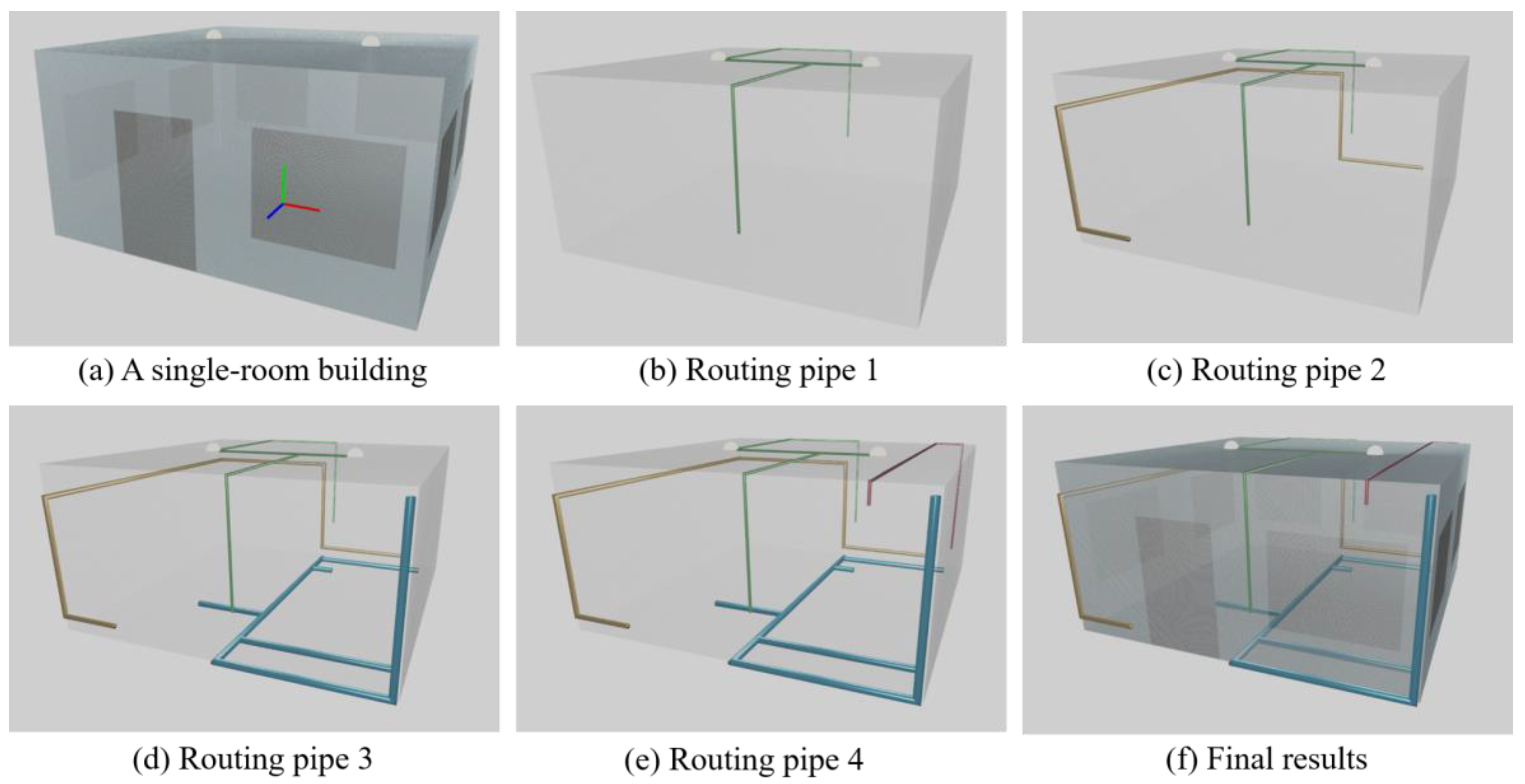
The appearance of the first building is shown in Figure 7a. Its dimensions, slabs, and openings are depicted in Table 1. It has four walls, one ceiling, and one floor. The thickness of these slabs is 30 cm. In the experiment, the slabs are decomposed into 1 cm × 1 cm × 1 cm voxels. Thus, a slab contains 10 layers of voxel planes. We use this model to simulate the piping process in a simple factory.
Four concealed pipes are to be routed in the building. Their basic parameters and applications are listed in Table 2. They are used for transferring electricity, gas, water, and air. Their diameters are 3, 6, 8, and 3 cm, respectively. The cross-sections of these pipes occupy at least 9 voxels and at most 64 voxels. In order to meet safety regulations, a pipe must be separated from other pipes by a certain distance. This distance is called the safe gap, which is enforced by using ε1 in Equation (1). This safe gap is maintained in only the plane of the slab that the pipe penetrated. Hence, it is a 2D distance regulation. If we select a large ε2 when creating the feasible spaces, the feasible spaces are enlarged and allow the pipes to deviate from existing obstacles and hazards further, and more space will be engaged in the routing calculation. The safe gaps of the pipes are shown in the fifth column of Table 2.
The progression of the routing process is shown in Figure 7b–e. In these images, the slabs are rendered as transparent grey polygons, and the pipes are shaded as solid and colorful tubes. Pipe 1 is arranged first. Its appearance is shaded green and is shown in Figure 7b. This pipe has four terminals located at the front and back walls and the ceiling. These terminals will be used for installing light bulbs and electrical switches. We use white balls to represent the light bulbs. The next pipe to be routed is pipe 2. Its path is shown in Figure 7c. We render it using orange. It has three terminals, but the resultant path contains only one branch. This is because its initial skeleton passes the third terminal, and thus no extra branch is needed to connect the third terminal.
The third pipe is the water pipe. It has six terminals and its diameter is the largest. Its path is rendered in blue and displayed in Figure 7d. Its path contains many branches such that the six terminals can be successfully connected. Its branches are mainly created on the floor because all terminals except one are located there. The last pipe to be routed is the air-conditioning pipe. It has only two terminals. Its path is shown in Figure 7e. As the image shows, its source and destination are at the back and front walls. Its path has to be routed inside the ceiling to connect these two terminals since the workspace in the floor has been occupied by the third pipe.
In order to display the 3D positions of these pipes in the building and to examine the quality of the pipe paths, a virtual reality image is produced to reveal the final scenario of the working environment. The pipes are portrayed using a surface-rendering subroutine while the slabs are drawn using a volume-rendering procedure. The final image is displayed in Figure 7f. As the image shows, the pipes do not cause any collisions with the obstacles (including the door, other pipes, and the windows) and their paths are hidden inside the slabs. The image also reveals that the pipe paths contain very few bends. This is caused by the penalty given in Equation (2). Furthermore, the gaps between the pipes are wide enough to meet safety regulations.
3.4. Test Case 2
In the next experiment, we build an apartment building and use it as the target building. Its appearance is shown in Figure 8a. The geometric information of this building is presented in Table 3. It has two units, and each unit is a two-story apartment. In a unit, the upper and lower stories are connected via a staircase. We created 11 windows in total on the front, back, and side walls in each unit. There is a window and a door between the two units on the second floor. Thus, these two units are connected. Each unit has a door in its front or side wall. In summary, the building has 20 slabs and 28 openings. Its size is 16 m × 16 m × 8 m. The shapes of the slabs and openings are presented in the second and third columns of Table 3.
Four concealed pipes are to be built. Their parameters are listed in Table 4. They are used to transport electricity, natural gas, water, and air. The first pipe possesses 18 terminals. The second pipe has 15 terminals. The third and fourth pipes have eight terminals and four terminals, respectively. The safety gaps and colors of the pipes are 20, 10, 5, and 2 cm, respectively.
Compared with the building model of test case 1, this building has more slabs and openings, and the target pipes possess more terminals too. Hence, the geometrical complexity of the working environment is greatly increased.
Figure 8b–e show the progression of the pipe routing process. The first pipe is shown in Figure 8b. Its path is confined within the ceilings and walls of the first and second stories. Its path contains some bends caused by the openings. However, most of its segments are straight. The second pipe is constructed subsequently, and its path is displayed in Figure 8c. A great portion of its path goes through the floors. This is because most of its terminals reside on the first floors and the slabs in the upper story are already occupied by the first pipe.
The path of the third pipe (in orange color) is portrayed in Figure 8d. Its path wanders through the spaces left by the first pipe in the upper story. It penetrates the back walls and ceilings to connect the terminals. The fourth pipe is the last to be routed. The remaining workspace is mostly in the front walls. Thus, its path is arranged in the front walls. Its path is shaded in red color and shown in Figure 8e. Figure 8f presents a VR image of the building after the piping process. It reveals the related positions of the pipes inside the building.
Our system can produce three-view images to highlight the gaps between the pipes and the spaces between the pipes and the openings. In Figure 9a–c, the orthographical projections of the building and the pipes are shown. These images are generated using the x-, y-, and z-axis projections. Based on Figure 9a, we can see that the pipes do not collide with any window or door. The image in Figure 9b verifies that the pipes do not go through the spaces used by the stair openings. Figure 9c shows the relative positions of the pipes to the windows in the front and back walls. No collision or violation of safety regulations is found.
3.5. Quantitative Data of the Tests
The lengths and routing costs of the pipes in both test cases are shown in Table 5. For each test, we present the ID of each pipe, the number of terminals in each pipe, the length of each pipe, and the computational time (wall-clock time measured in seconds.).
Since the second building is larger and more complicated, routing pipes in its slabs is expected to be more time-consuming and the pipe lengths would be longer. The data shown in Table 5 match our expectations. By examining the number of terminals and the length and routing cost of each pipe, we found that the number of terminals is the major factor influencing the routing time. This phenomenon is more obvious in test 1. The minor factor affecting the execution time is the pipe length. For example, the third pipe of test 2 has only eight terminals but its length is relatively long and its routing cost is higher.
The other important factor in deciding the cost is the order of pipe. In test 2, the first pipe has more terminals and its path is longer, compared with pipe 3. However, its piping cost is lower. This is because this pipe is arranged first, its feasible space is simple, and less computer time is consumed for searching the path directions and creating the branches. If we compare images Figure 8b,d, the first pipe has fewer branches than the third pipe. This property reflects the importance of the pipe scheduling process.
4. Discussion and Future Work
Pipe routing algorithms can be characterized by their working environments, routing algorithms, data structures, and applications. In Table 6, we list some typical pipe-routing research and our work and characterize these methods by using the above factors such that the differences among them can be highlighted.
Based on our investigation into the literature, many researchers use Dijkstra’s method and the A* algorithm to find the pipe paths. In their work, workspaces are usually encoded using weighted graphs. However, their applications may be very different. The ACO algorithm and its variants are the second most popular approaches for laying out pipes. Their underlying data structures may be grids or weighted graphs. ACO methods are utilized to find optimal solutions for routing problems with multiple pipes.
To our knowledge, there is no research focusing on the routing process inside building slabs. Ours might be the first one. Furthermore, to increase computational efficiency, the proposed method adopts a hierarchical data structure to encode the workspace and a two-stage piping method to arrange the pipe paths. The embedded routing approach and data structure are also different from those adopted by the other researchers. However, our target application is not unique and is similar to those of [6,14,15,16,17]. The proposed piping method is utilized for laying our MEB systems, though the conduits are concealed by the walls, floors, and ceilings of buildings.
In this research, the pipe paths contain only straight segments and 90-degree elbows. In reality, 45-degree bends should be allowed in pipe paths. We believe the execution time and the quality of the piping process might be improved by relaxing the restriction of the bend angle, especially for pipes relying on gravity to deliver materials.
By examining the images of Figure 7 and Figure 8, we found that the pipe paths are closer to the boundaries of the slabs. This is because we utilized Equation (1) to form the feasible space. Therefore, the feasible space of the first pipe is adjacent to the slab boundaries and the openings. Then, the first pipe becomes an obstacle, and the distance field is renewed. Next, the feasible space of the second pipe is created adjacent to the slab boundaries and openings as well as the first pipe. This strategy has a ripple effect. The following pipes will be routed within a safe but not far distance from the slab boundaries, openings, and existing pipes. The safety regulations are met, but large spaces may be preserved in the middle portions of the slabs. This aspect is beneficial for exposed conduits because less space is used and the pipes are closer to supporting racks, which are usually built near the surfaces. We believe that it is also good for concealed pipes since users can obtain more free space for drilling the slabs to install hangers or other facilities.
Additive Manufacturing (AM) has been proposed to construct buildings [23]. Creating tunnels in slabs manufactured by AM processes will allow users to route electricity wires and computer network cables afterward. Thus, the proposed algorithm can be employed to create concealed pipes in the geometric modeling stages of AM processes. Another potential application of the proposed method is to design tunnels in cooling jackets, especially incorporated with AM technology [24]. The tunnels of a cooling jacket are concealed inside the walls of the jacket. Filled with running liquids, they are used to transfer the heat produced by electronic devices or machines. Their application is different from the concealed pipes in a building. However, their geometric characteristics are similar to those of the concealed pipes. By using the concept of the distance field and voxelization process, the proposed method is suitable for routing cooling tunnels.
5. Conclusions
This article presents an innovative routing method for concealed pipes. The proposed algorithm encodes the workspace in a two-level structure. The top-level representation records the slabs and the connectivity relations of the slabs in a weighted graph. In the bottom-level representation, the workspace is converted into a set of 3D images of voxels such that the distance field computation, voxel labeling, and feasible space creation are simplified. The proposed method employs a two-stage routing procedure to lay out concealed pipes. In the first stage, the abstract paths of the target pipes are calculated in the top-level representation of the workspace. Then, in the second stage, the real pipe path of each pipe is computed in the bottom-level representation. Thus, an exhaustive search is not required for routing the pipe. The proposed piping procedure creates a feasible space for routing the path of each pipe. The feasible space is free of any collision and meets all safety regulations and geometric constraints. Thus, the computational costs are further reduced, and the quality of the piping process is guaranteed.
We perform experiments to verify the effectiveness of the proposed piping method. Two test results are presented by using qualitative and quantitative methods. Our piping system displays the intermediate results at the run-time by using surface rendering and volume rendering. The resultant images enable users to visually examine the quality of the pipes. Moreover, we present the computational costs and lengths to express the quantitative data of the experiments. By analyzing these data, we conclude that the costs of the piping process are mainly influenced by the number of terminals, the lengths, and the orders of the pipes.
As AM techniques are gaining popularity in manufacturing and construction applications, we propose to incorporate the proposed method with AM technology for building houses and making mechanic components in the future.
Author Contributions
Conceptualization, S.-K.U.; methodology, S.-K.U.; software, C.-C.C..; validation, S.-K.U. and C.-C.C.; formal analysis, S.-K.U.; investigation, C.-C.C.; data curation, C.-C.C.; writing—original draft preparation, S.-K.U.; writing—review and editing, S.-K.U.; visualization, C.-C.C.; supervision, S.-K.U.; project administration, S.-K.U.; funding acquisition, S.-K.U. All authors have read and agreed to the published version of the manuscript.
Funding
MOST Taiwan, grant number 109-2221-E-019-055.
Institutional Review Board Statement
Not applicable.
Informed Consent Statement
Not applicable.
Data Availability Statement
Not applicable.
Acknowledgments
This research was funded by MOST Taiwan, grant number 109-2221-E-019-055.
Conflicts of Interest
The authors declare no conflict of interest.
References
- Qian, X.L.; Ren, T.; Wang, C.E. A Survey of pipe routing design. In Proceedings of the Chinese Control and Decision Conference, Yantai, China, 2–4 July 2008; pp. 3994–3998. [Google Scholar]
- Lee, C.Y. An algorithm for path connections and its applications. IRE Trans. Electron. Comput. 1961, 3, 346–365. [Google Scholar] [CrossRef]
- Kim, S.; Kim, S.; Choi, T.; Kwon, T.; Lee, T.H.; Lee, K. Automatic design system for generating routing layout of tubes, hoses, and cable harnesses in a commercial truck. J. Comput. Des. Eng. 2021, 8, 1098–1114. [Google Scholar] [CrossRef]
- Ueng, S.K.; Huang, H.K. A distance-field-based pipe-routing method. Materials 2022, 15, 5376. [Google Scholar] [CrossRef] [PubMed]
- Asmara, A.; Nienhuis, U. Automatic piping system in ship. In Proceedings of the International Conference on Computer and IT Application (COMPIT), Leiden, The Netherlands, 8–10 May 2006; pp. 269–280. [Google Scholar]
- Choi, W.; Kim, C.; Heo, S.; Na, S. The modification of A* pathfinding algorithm for building mechanical, electronic and plumbing (MEP) path. IEEE Access 2022, 10, 65784–65800. [Google Scholar] [CrossRef]
- Gao, H.; Koch, C.; Wu, Y. Building information modelling based building energy modelling: A review. Appl. Energy 2019, 238, 320–343. [Google Scholar] [CrossRef]
- Xie, H.; Tramel, J.M.; Shi, W. Building information modeling and simulation for the mechanical, electrical, and plumbing systems. In Proceedings of the IEEE International Conference on Computer Science and Automation Engineering, Shanghai, China, 10–12 June 2011; pp. 77–80. [Google Scholar]
- Horowitz, E.; Sahni, S.S.; Rajasekaran, S. Computer Algorithm; Computer Science Press: New York, NY, USA, 1998. [Google Scholar]
- Qu, Y.F.; Jiang, D.; Zhang, X.L. A new pipe routing approach for aero-engines by octree modeling and modified max-min ant system optimization algorithm. J. Mech. 2018, 34, 11–19. [Google Scholar] [CrossRef]
- Ito, T. A genetic algorithm approach to piping route path planning. J. Intell. Manuf. 1999, 10, 103–114. [Google Scholar] [CrossRef]
- Kang, S.S.; Sehyun, M.; Hah, S.H. A design expert system for auto-routing of ship pipes. J. Ship Prod. 1999, 15, 1–9. [Google Scholar] [CrossRef]
- Christodoulou, S.E.; Ellinas, G. Pipe routing through ant colony optimization. J. Infrastruct. Syst. 2010, 16, 149–159. [Google Scholar] [CrossRef]
- Zhang, N.; Wang, J.; Al-Hussein, M.; Yin, X. BIM-based automated design of drainage systems for panelized residential buildings. Int. J. Constr. Manag. 2022, 1–16. [Google Scholar] [CrossRef]
- Samarasinghe, T.; Gunawardena, T.; Mendis, P.; Sofi, M.; Aye, L. Dependency Structure Matrix and Hierarchical Clustering based algorithm for optimum module identification in MEP systems. Autom. Constr. 2019, 104, 153–178. [Google Scholar] [CrossRef]
- Farooq, J.; Sharma, P. Applications of Building Information Modeling in Electrical Systems Design. J. Eng. Sci. Technol. Rev. 2017, 10, 119–128. [Google Scholar] [CrossRef]
- Teo, Y.H.; Yap, J.H.; An, H.; Yu, S.C.M.; Zhang, L.; Chang, J.; Cheong, K.H. Enhancing the MEP Coordination Process with BIM Technology and Management Strategies. Sensors 2022, 22, 4936. [Google Scholar] [CrossRef] [PubMed]
- Yue, Y.; Liu, Z.; Zuo, X. Integral layout optimization of subsea production control system considering three-dimensional space constraint. Processes 2021, 9, 1947. [Google Scholar] [CrossRef]
- Liu, M.Y.; Tuzel, O.; Veeraraghavan, A.; Chellappa, R. Fast directional chamfer matching. In Proceedings of the IEEE Conference on Computer Vision and Pattern Recognition, San Francisco, CA, USA, 13–18 June 2010; pp. 1696–1703. [Google Scholar]
- Sethian, J.A. Fast marching methods. SIAM Rev. 1999, 41, 199–235. [Google Scholar] [CrossRef]
- Ueng, S.K.; Huang, H.C.; Chou, C.S.; Huang, H.K. Layered manufacturing for medical imaging data. Adv. Mech. Eng. 2019, 11. [Google Scholar] [CrossRef]
- Kaufman, A.; Dachille, F.; Chen, B.; Bitter, I.; Kreeger, K.; Zhang, N.; Tang, Q. Real-time volume rendering. Int. J. Imaging Syst. Technol. 2000, 11, 44–52. [Google Scholar] [CrossRef]
- Tay, Y.W.D.; Panda, B.; Paul, S.C.; Noor Mohamed, N.A.; Tan, M.J.; Leong, K.F. 3D printing trends in building and construction industry: A review. Virtual Phys. Prototyp. 2017, 12, 261–276. [Google Scholar] [CrossRef]
- Szabó, L. Survey on applying 3D printing in manufacturing the cooling systems of electrical machines. In Proceedings of the 2022 IEEE International Conference on Automation, Quality and Testing, Robotics (AQTR), Cluj-Napoca, Romania, 19–21 May 2022; pp. 1–6. [Google Scholar]
Figure 1.
(a) Exposed conduits and (b) concealed conduits. The exposed conduits are built in open spaces or on the surfaces of objects while the concealed conduits are constructed inside the walls, ceilings, and floors of a building. The working domain of concealed conduits is more complicated, and the routing process would be challenging.

Figure 2.
Overview of the proposed concealed pipe routing method.

Figure 3.
The framework of a building is composed of beams, columns, and slabs. The red, green and blue lines represent the x-, y- and z-axes.
Figure 3.
The framework of a building is composed of beams, columns, and slabs. The red, green and blue lines represent the x-, y- and z-axes.

Figure 4.
Top-level representation of a simple building: (a) The building, (b) the weighted graph of the top-level representation (the weights are not revealed).
Figure 4.
Top-level representation of a simple building: (a) The building, (b) the weighted graph of the top-level representation (the weights are not revealed).

Figure 5.
The bottom level of the hierarchical representation is composed of 3D images (slabs).

Figure 6.
Flowchart of the pipe-routing computation. The key computations include abstract path routing, pipe scheduling, pipe path finding, pipe surface modeling, and workspace updating steps.
Figure 6.
Flowchart of the pipe-routing computation. The key computations include abstract path routing, pipe scheduling, pipe path finding, pipe surface modeling, and workspace updating steps.

Figure 7.
Routing concealed pipes in a single-room building, (a) the building, (b–e) routing pipe 1–4, (f) the resultant pipe systems.
Figure 7.
Routing concealed pipes in a single-room building, (a) the building, (b–e) routing pipe 1–4, (f) the resultant pipe systems.

Figure 8.
Routing concealed pipes in an apartment building, (a) the building, (b–e) routing pipe 1–4, (f) the resultant pipe systems.
Figure 8.
Routing concealed pipes in an apartment building, (a) the building, (b–e) routing pipe 1–4, (f) the resultant pipe systems.

Figure 9.
Three-view projections of the concealed pipes of experiment 2, (a) the side view, (b) the top view, and (c) the front view.
Figure 9.
Three-view projections of the concealed pipes of experiment 2, (a) the side view, (b) the top view, and (c) the front view.


Table 1.
Geometric information of the first test model.
| Dimension | Slabs | Opening |
|---|---|---|
| Width = 8 m, Length = 8 m, Height = 4 m | 4 walls (8 m × 4 m), 1 floor (8 m × 8 m), 1 ceiling (8 m × 8 m) | 1 door (1.8 m × 3 m), 7 windows (2 m × 2.6 m) |
Table 2.
Pipe parameters in test case 1.
| Pipe | #(Terminals) | Diameter | Usage | Safe Gap | Color |
|---|---|---|---|---|---|
| 1 | 4 | 3 cm | Electricity | 20 cm | Green |
| 2 | 3 | 6 cm | Natural gas | 10 cm | Orange |
| 3 | 6 | 8 cm | Water | 5 cm | Blue |
| 4 | 2 | 3 cm | Air | 2 cm | Red |
Table 3.
Geometric information of the building in the second test.
| Components/Dimensions | Slabs | Opening |
|---|---|---|
| Apartment of 2 units, 2 stories in 1 unit, Width = 16 m, Length = 16 m, Height = 8 m, 4 rooms. | 20 slabs: 14 (8 m × 4 m) walls, 4 (8 m × 8 m) floors, 2 (8 m × 8 m) ceilings. Slab thickness = 30 cm. | 3 (1.8 m × 3 m) doors: 2 doors in 1st floor, 1 door in the 2nd floor. 23 (2 m × 2.6 m) windows: 11 windows in the 1st floor, 12 windows in the 2nd floor. 2 (4 m × 2 m) staircase openings, 1 opening in each unit. |
Table 4.
Pipe parameters in test case 2.
| Pipe | #(Terminals) | Diameter | Usage | Safe Gap | Color |
|---|---|---|---|---|---|
| 1 | 18 | 3 cm | Electricity | 20 cm | Green |
| 2 | 15 | 6 cm | Natural gas | 10 cm | Orange |
| 3 | 8 | 8 cm | Water | 5 cm | Blue |
| 4 | 4 | 3 cm | Air | 2 cm | Red |
Table 5.
Lengths and routing costs of the pipes in the 2 tests.
| Pipe | Test 1 | Test 2 | ||||
|---|---|---|---|---|---|---|
| #(Terminals) | Length (m) | Cost (sec.) | #(Terminals) | Length (m) | Cost (sec.) | |
| 1 | 4 | 19.92 | 2.59 | 18 | 75.53 | 13.83 |
| 2 | 3 | 22.30 | 1.30 | 15 | 54.68 | 10.37 |
| 3 | 6 | 25.00 | 3.15 | 8 | 72.42 | 19.69 |
| 4 | 2 | 12.56 | 0.40 | 4 | 25.78 | 2.20 |
Table 6.
Comparisons among various piping research.
| Researches | Routing Algorithms | Data Structures | Working Environment | Applications |
|---|---|---|---|---|
| Kim et al. [3] | Genetic algorithm | Graph | Vehicles | Cables & pipes of vehicles |
| Choi et al. [6] | A* method | Graph | Buildings | MEB systems |
| Qu et al. [10] | ACO algorithm | Octree | Engine surfaces | Aero-engine pipes |
| Kang et al. [12] | Expert system | Graph | Ships | Pipes of ships |
| Christodoulou [15] | ACO algorithm | Graph | Communities | Water supply systems |
| Ours | Two-stage Dijkstra method | Graph + 3D voxel images | Building slabs | MEB systems |
Disclaimer/Publisher’s Note: The statements, opinions and data contained in all publications are solely those of the individual author(s) and contributor(s) and not of MDPI and/or the editor(s). MDPI and/or the editor(s) disclaim responsibility for any injury to people or property resulting from any ideas, methods, instructions or products referred to in the content. |
© 2023 by the authors. Licensee MDPI, Basel, Switzerland. This article is an open access article distributed under the terms and conditions of the Creative Commons Attribution (CC BY) license (https://creativecommons.org/licenses/by/4.0/).
Share and Cite
MDPI and ACS Style
Ueng, S.-K.; Chang, C.-C. Concealed Conduit Routing in Building Slabs. Appl. Sci. 2023, 13, 10847. https://doi.org/10.3390/app131910847
AMA Style
Ueng S-K, Chang C-C. Concealed Conduit Routing in Building Slabs. Applied Sciences. 2023; 13(19):10847. https://doi.org/10.3390/app131910847
Chicago/Turabian StyleUeng, Shyh-Kuang, and Chun-Chieh Chang. 2023. "Concealed Conduit Routing in Building Slabs" Applied Sciences 13, no. 19: 10847. https://doi.org/10.3390/app131910847
Note that from the first issue of 2016, this journal uses article numbers instead of page numbers. See further details here.