Application of Vehicle-Based Indirect Structural Health Monitoring Method to Railway Bridges—Simulation and In Situ Test

Abstract

In recent years, the vehicle-based indirect Structural Health Monitoring (iSHM) method has been increasingly used to identify the dynamic characteristics of railway bridges during train crossings, and it has been shown that this method has several advantages compared to traditional SHM methods. A major advantage is that sensors are just mounted on the vehicle, and no sensors or data acquisition systems need to be installed on the railway bridge. In this paper, the application of the vehicle-based iSHM method is demonstrated numerically and experimentally for determining the natural frequencies of railway steel bridges during train crossing. The coupled linear equations of motion of the train-bridge multi-body system are derived, and train crossing simulations are conducted numerically, considering different train speeds. Three different railway bridges are considered, and the train-induced vibration responses are calculated for both the train multi-body system and the railway bridge models. Different representative evaluation points are chosen for the wheelsets, bogies, and car bodies of the considered vehicle. To calibrate the numerical model, the resonance frequencies of an existing single-span steel bridge are measured in situ by the application of forced vibration tests. Besides the executed in situ measurements of the bridge, the considered crossing vehicle is also instrumented with several accelerometers at the wheelsets, bogies, and car bodies, and the vibration responses of both the bridge and the crossing vehicle are measured simultaneously during the duration of several train crossings with different train speeds. The recorded vibration responses are analyzed in the frequency domain and compared with numerical simulation results. It is shown that the first bending frequency of the considered railway bridge can be clearly identified from the computed frequency response spectra and that the vehicle-based iSHM method provides a promising tool for identifying the dynamic characteristics of railway bridges.

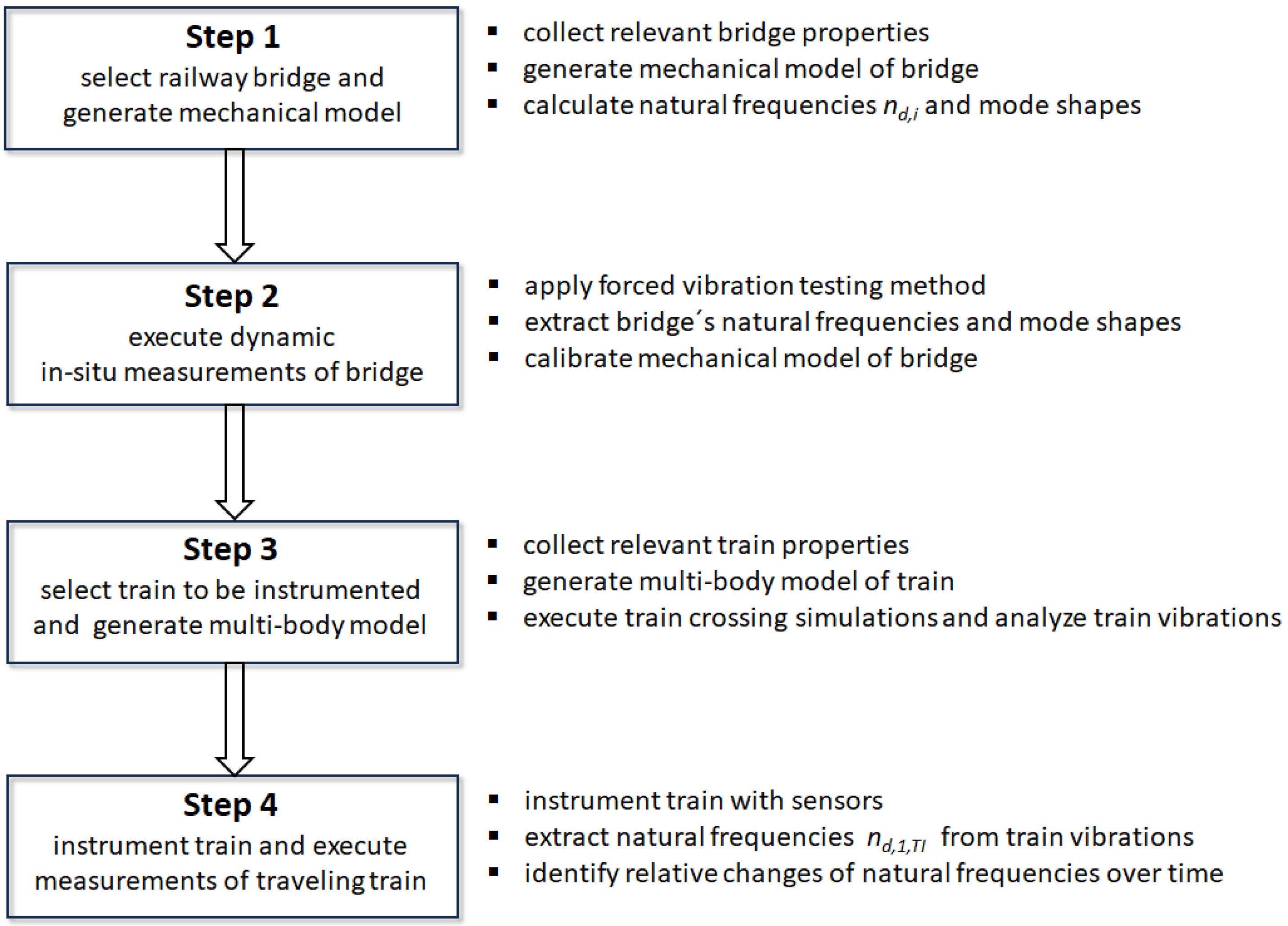
1. Introduction

Railway bridges are excited to forced vibrations during train crossings, which can lead to a destabilization of the ballast bed, especially in the case of resonance excitation [1]. Thus, instability of the rail position may occur, eventually leading to safety issues for trains and passengers, respectively. Generally, in the case of designing new railways and operational planning of existing bridges, for example, due to the introduction of new rolling stock or an increase in operational speed, a computational verification of serviceability must be carried out. In this context, it must be verified that the maximum occurring vertical bridge deck accelerations do not exceed the limit accelerations specified in the standards, the Eurocode EN 1990:2002/A1:2005/AC:2010 [2], and additionally, on a national level, the RW 08.01.04 [3] to be applied in Austria, in order to exclude any possible risk to the longitudinal, transversal and vertical track stability, the fatigue strength of the supporting structures, and the riding comfort in passenger traffic, or the storage safety regarding freight traffic.

The forced vibration responses of railway bridges depend dominantly on the bridge’s natural frequencies and damping characteristics. Resonance vibrations occur if one of the trains crossing excitation frequencies meets one of the bridge’s eigenfrequencies, and they are associated with detrimental large vibration amplitudes [4,5]. Hence, the knowledge of the bridge’s natural frequencies is vital to evaluate train-induced vibrations and to ensure the bridge’s serviceability.

To determine the natural frequencies of existing bridges, classical in situ measurement methods, such as the ambient vibration test [6], forced vibration test [7], impact vibration test [8], and train excitation test [9] have been frequently applied. These classical measurement methods are often referred to as the direct approach since they usually require many sensors directly installed in the bridge structure. Contrary to the classical time-consuming in situ measurement methods, Yang et al. [10] proposed to determine the natural frequencies of a road bridge from the measured dynamic response of crossing vehicles and later verified the proposed method through in situ tests [11]. The proposed technique, named vehicle-based indirect Structural Health Monitoring (iSHM) or ‘drive-by’ bridge SHM, provides a promising method, namely by using the indirect measurements from a moving vehicle [12,13,14,15,16,17].

The approach uses sensors that are installed on traveling vehicles to collect the bridge response during the train crossing event, which is referred to as the indirect method of bridge response measurements. In comparison to conventional bridge SHM, the concept of vehicle-based iSHM shows many advantages in terms of being low-cost, time-saving, and highly efficient. Therefore, this method has recently received extensive attention and achieved great development. However, currently, no regulation and/or standard exists for the application of the iSHM method. Most related investigations focus on extracting the bridge’s dynamic properties with indirect measurements of train vibrations, i.e., natural frequencies [18,19,20,21,22,23], damping ratios [24,25,26], and mode shapes [27,28,29,30,31]. The change of those modal properties is frequently used for bridge damage detection [32,33,34,35,36,37].

However, in the application of the vehicle-based iSHM method to railway bridges, several challenges arise in extracting the natural frequencies, corresponding mode shapes, and damping ratios from the recorded sensor signals. For instance, the span lengths of railway bridges are typically very short (below 20 m), and the trains cross the bridge at high speed, which implies that the duration of the vehicle traveling on the bridge is very short and the sensor signals recorded from the crossing vehicle are often not long enough for the application of a reliable signal processing method to extract the bridge’s natural frequencies with the desired accuracy. Hence, to obtain the best accuracy for estimating the bridge’s natural frequencies, most of the studies consider the crossing vehicles at low speed, as pointed out by Lin and Yang [11]. However, Zhan et al. [38] presented a new method to identify the bridge frequency from vehicles moving at high speed by combining the responses of multiple vehicles. It is shown that by combining the acceleration of several vehicles to extend the overall duration of the signal, the frequency resolution can be improved, and the bridge frequency can be successfully identified using vehicles traveling at high speed. However, currently, no regulations and/or standards exist for the application of the iSHM method, and currently, it is noted that almost all articles on the application of the iSHM method are based on theoretical studies and numerical simulations of the traveling train and bridge, respectively. Results of in situ measurements with instrumented trains and railway bridges and their comparison with theoretical and numerical simulation results are often missing part in scientific studies.

Hence, the objective of this paper is to present the application of the vehicle-based iSHM method to extract the first bending frequency of railway bridges and to validate the results of numerical simulations by in-situ measurements of both the train and bridge vibrations during the train crossing events. In the first part of the paper, the theoretical train and bridge model is presented based on the vehicle–bridge interaction model composed of a two-dimensional multi-body system of eleven coaches interconnected through Jacobs bogies and a simply-supported Euler–Bernoulli beam. In the second part, besides numerical simulations of train crossings with different train speeds and analyzing the computed vibration responses in the frequency domain, in situ tests are conducted to validate the results of the numerical simulation. Both the considered steel deck bridge and the crossing train are, therefore, instrumented with several accelerometers, and the vibration responses are measured during train crossing. The results of numerical simulations and in situ tests are presented and compared. Finally, some conclusions will be given based on the conducted theoretical and experimental research work.

Figure 1 illustrates the entire process applied in our research to extract natural frequencies of railway bridges—after first determination through forced vibration testing—from train recorded data only.

2. Dynamic Modeling of Bridge Structure and Crossing Train

Calculating the structural and train vibrations requires idealizing the dynamic system of the train crossing the bridge as a mechanical model, for which the system of coupled equations of motion can be set up and solved numerically. In principle, reality is best represented with a high complexity of the mechanical model, i.e., with a multi-body dynamic system including beneficial interaction effects between all vibrating components. However, this also requires knowledge about the numerous elements of the supporting structure, the track, and the crossing train, as well as their interaction. Information about high-speed trains, in particular, is rarely publicly available due to the confidentiality policies of the train manufacturers. Furthermore, with the complexity of the applied models, the computational effort also increases significantly. Within the scope of the following investigations, relatively simple mechanical models were used, the essential aspects of which are briefly described below. Detailed information on the models can be found in [39,40,41,42,43,44,45], among others.

2.1. Mechanical Model of the Bridge Structure

The bridge structure is modeled as a simply-supported single-span girder (a shear-rigid Euler–Bernoulli beam) with a span length of L, where the beam’s properties summarize all structure properties, including the track. The load-distributing effect of the track itself and the interaction dynamics between the structure and the rails, e.g., possible energy dissipation capacities and the restraining effect at the ends of the structure, are neglected.

The beam’s bend line w_B(x,t) can be approximated by modal analysis for n considered vibration modes as follows:

$$w_{\mathrm{B}}\left(x,t\right)\approx \sum _{i=1}^n{q}_i\left(t\right)\cdot {\varphi }_i\left(x\right),n=5.$$

(1)

Five vibration modes with corresponding shape functions ϕ_i(x) = sin(i π x/L) and generalized displacements q_i(t) are considered in the computational investigations. The system of linear equations of motion for the generalized displacements q_i(t) of the bridge structure then follows:

$${\mathit{M}}_{\mathbf{B}}\ddot{\mathit{q}}+{\mathit{C}}_{\mathbf{B}}\dot{\mathit{q}}+{\mathit{K}}_{\mathbf{B}}\mathit{q}={\mathit{p}}_{\mathbf{B}}.$$

(2)

The modal mass, damping, and stiffness matrices M_B, C_B, and K_B on the left side of Equation (2) contain information on the bridge’s span L, bending stiffness EI$,$ mass distribution per unit length μ, and Lehr’s damping factor ζ (by applying Rayleigh damping), the latter two including the contribution of the (in the case of the investigations described) ballasted track. This mechanical model allows only consideration of vertical bending deformations due to the generalized external load vector p_B. Shear deformations and horizontal and torsional vibrations are omitted; the latter would require applying a three-dimensional model of the bridge structure.

As previously stated, verifying the compliance of occurring vertical bridge deck accelerations with the normative limits is mandatory for new and existing constructions, whereby the accelerations often become a decisive criterion. This article focuses on the dynamic assessment of a specific existing steel deck bridge in Austria (see Section 3.1 and Section 4.1). Its properties, on which the following evaluations are based, are summarized in

Table 1. Bridge properties of the considered existing steel deck bridge required for dynamic calculation.

L [m]	EI [Nm2]	ζ [%]	nd,1 [Hz]	μ [kg/m]	μ’ [kg/m]	μtrack [kg/m]
33.3 (1)	73.18 × 109 (1)	1.88 (2)	4.52 (2)	7188 (3)	3587 (1)	3601

⁽¹⁾ from planning documents and in situ geometric cross-section measurements; ⁽²⁾ from in situ vibration measurements (forced vibration tests with shakers, bandwidth analysis), see Section 4.2; ⁽³⁾ recalculated from the relation: $\mu =EI{\left(\frac{\pi }{2n_1{L}^2}\right)}^2$ assuming n₁ ≈ n_d,1 for ζ < 10%.

. The resonance frequency n_d,1 of the first bending mode, and the structural damping factor ζ were determined by executing in situ measurements described in the following Section 4.2. In the first step, the bending stiffness EI was estimated from the structure’s cross-section using technical drawings and additional geometric site measurements. The bending stiffness was adequately adjusted in the second step to obtain a good agreement between the measured calculated first resonance frequency and the calculated frequency. Finally, the mass distribution per unit length μ was recalculated with the relation $\mu =EI {\left(\frac{\pi }{2 n_1 L^2}\right)}^2$, which can be applied to simply-supported beam structures, assuming the natural frequency n₁ is approximately the resonance frequency n_d,1 for small structural damping factors of ζ < 10%. The comparison of μ with the mass distribution μ’, which denotes only the mass of the steel structure and additional mounted elements, e.g., the cantilever steel construction with fastened noise barrier, allows an estimation of the mass distribution of the track μ_track = 3601 kg/m (rails, sleepers, and ballast bed). Assuming a mass distribution of 120 kg/m for the rails, 300 kg of concrete sleepers every 0.6 m (corresponding to 500 kg/m), and a ballast bed cross-section of 2.07 m² (at a ballast bed height of 0.55 m of the standardized superstructure in Austria), this results in an approximate ballast density of 1440 kg/m³.

To evaluate whether it is possible to apply the proposed vehicle-based iSHM method for determining dynamic bridge parameters via analyzing the vibration response of the crossing train, numerical calculations are additionally also performed for two fictitious bridges. Their assumed dynamic characteristics are summarized in

Table 2. Bridge properties of two additional fictitious bridge structures for dynamic calculation.

No.	L [m]	EI [Nm2]	ζ [%]	n1 [Hz]	μ [kg/m]
1	11.0	5.70 × 109 (3)	1.63 (2)	11.51 (1)	7253 (1)
2	5.0	1.64 × 109 (3)	2.55 (2)	23.17 (1)	12,040 (1)

⁽¹⁾ from analyses of the catalog of existing bridges [39,44,45]; ⁽²⁾ from EN 1991-2:2003 [46]; ⁽³⁾ recalculated from the relation: $EI=\mu {\left(\frac{2n_1{L}^2}{\pi }\right)}^2$.

. Natural frequency n₁, span length L, and mass distribution μ are defined by analyzing the properties of 275 existing single-span and single-track bridges in the European rail network (see [39,44,45]) and correspond to a medium-span steel bridge and a short-span concrete bridge. Lehr’s damping ratio ζ is taken from the applicable standards, the Eurocode EN 1991-2:2003 [46], which prescribes span- and construction type-dependent lower bound functions. The bending stiffness is recalculated by rearranging the previous Equation for the mass distribution to $EI=\mu {\left(\frac{2 n_1 L^2}{\pi }\right)}^2$.

2.2. Mechanical Model of Train

The dynamic excitation is generated by the articulated train moving over the bridge at a constant speed. It is modeled as a two-dimensional multi-body system of eleven coaches interconnected through Jacobs bogies, see Figure 2. Two driving directions were considered, hereafter referred to as driving directions toward Vienna or Salzburg. It is noted that the first car of the considered vehicle in the Vienna driving direction is always denoted c1. Therefore, depending on the driving direction of the train, the order in which the cars and bogies arrive on the bridge changes, i.e., in the case of the Vienna train driving direction, car c1 and bogie b1 arrive first, and in the case of the Salzburg driving direction, car c11 and bogie b12 arrive first on the bridge.

Car bodies, bogie frames, and wheelsets are modeled as rigid bodies with mass inertia and one vertical and one rotational degree of freedom (DOF) each (besides the wheelsets with only vertical DOFs). All train components are coupled with linear spring-damper elements representing the train’s primary and secondary suspension system. In addition to Equation (2), the following second equation of motion for the kinematics of the vehicle multi-body system must be solved in each time step:

$${\mathit{M}}_{\mathbf{V}}\ddot{\mathit{u}}+{\mathit{C}}_{\mathbf{V}}\dot{\mathit{u}}+{\mathit{K}}_{\mathbf{V}}\mathit{u}={\mathit{F}}_{\dot{\mathbf{W}}}+{\mathit{F}}_{\mathbf{W}}.$$

(3)

The properties of the car bodies, bogies, and primary and secondary suspensions (see Figure 1) are included in the mass, damping, and stiffness matrices M_V, C_V, and K_V. The vector u and its time derivatives $\dot{\mathit{u}}$ and ü consist of the previously mentioned DOFs of all trains’ car bodies and bogie frames. The DOFs of the wheelsets, i.e., their vertical displacement w_W,j(t) at any time t of the train crossing (cf. Figure 2), can be extracted from the equation of motion of the train by equating them with the vertical bridge displacement w_B(x_j,t) at the respective wheel contact point. This assumed rigid and continuous contact between the bridge and wheelsets forms the coupling relation of both systems of equations of motion from Equations (2) and (3) as w_W,j(t) = w_B(x_j,t).

The dynamic interaction of the components of both subsystems, train and bridge structure, further leads to establishing both load vectors, the external load vector p_B in the system of equations of motion of the bridge structure, and the vectors F_W and F_Ẇ, acting on the systems of equations of motion of the train. The present investigations did not include rail or track irregularities, which could be simulated by implementing a power density function representing irregularities of various wavelengths to the load vectors of both systems of Equations (2) and (3), for instance, described in refs. [45,46,47,48,49].

The generalized load vector p_B in Equation (2) represents the contact forces transmitted from each wheelset w_j (j = 1, 2, …, m) to the bridge at its time-dependent location x_j; see also Equation (4). It contains the static axle load F_stat,j, the dynamic force components F_k,j and F_c,j transmitted in the primary suspension, and the inertia force of the wheelset m_W,j ẅ_W,j (t),

$${\mathit{p}}_{\mathbf{B}}=\sum _{i=1}^n\left(\sum _{j=1}^m\left[F_{\mathrm{s}\mathrm{t}\mathrm{a}\mathrm{t},j}-F_{\mathrm{k},j}\left(t\right)-F_{\mathrm{c},j}\left(t\right)-m_{\mathrm{W},j}{\ddot{w}}_{\mathrm{W},j}\left(t\right)\right]\mathsf{\Gamma }\left(x_j\right){\varphi }_i\left(x_j\right)\right).$$

(4)

Similarly, the load vectors in Equation (3) comprise the spring respectively damper forces F_W and F_Ẇ acting on each bogie frame. Additionally, the masses of the wheelsets of the train are included in the mass matrix of the bridge M_B with a time-dependent location. More detailed information regarding the multi-body vehicle model can be found, for instance, in refs. [39,40,41,42,43,44,45].

3. Dynamic Calculation of Bridge and Train Vibrations

3.1. Analyses of Considered Steel Bridge in Time Domain

The dynamic system’s vibrations are numerically calculated considering the speed range of the trains between 60 and 420 km/h, discretized in 1 km/h steps. The coupled systems of equations of motion of bridge structure and train are numerically integrated using the pre-implemented differential equation solvers in MATLAB 2022 [50], specifically with the algorithm ode15 s for stiff problems, which is based on the numerical differentiation formulas (NDFs), see for instance in ref. [51]. Critical and, therefore, design-relevant accelerations of the bridge mainly occur when the external excitation of the crossing train causes resonance vibrations. The characteristic resonance speeds v_crit,i, at which the excitation speed of regularly spaced axle loads with the spacing s = 17.5 m being defined as the car length of the considered vehicle, see Figure 2, equals the resonance frequency n_d,1 of the examined bridge structure, can be determined as follows:

$$v_{crit,i}=\frac{s\cdot n_{d,1}}{i} , i=1, 2, \dots$$

(5)

The bridge vibration responses induced by a crossing load can also be canceled out and thus feature significantly lower acceleration amplitudes than at other train speeds when the span- and natural frequency-dependent cancellations speeds v_canc,i according to [52] are reached:

$$v_{canc,i}=\frac{2\cdot L\cdot n_{d,1}}{2i-1} , i=1, 2, \dots$$

(6)

Resonance accelerations induced at critical speeds v_crit,i close to a cancellation speed v_canc,i are likely to be suppressed by the dominating cancellation effect.

From the dynamic calculations performed, the bridge accelerations at midspan, and the bogie frame and car body accelerations in proximity to three train couplings at the front (bogie frame b2—wheelset w3 and w4), end (bogie frame b11—wheelset w21 and w22) and one middle (bogie frame b6—wheelset w11 and w12) Jacobs bogie are read out as computation results. The bogie frame and car body vibrations are evaluated at the same distance from the bogie axes as in the in situ measurements (exemplarily shown in Figure 2), which means that the acceleration results include vibration components from vertical accelerations at each body’s center of gravity and rotational accelerations as defined below:

$${\ddot{w}}_{\mathrm{c},k,\mathrm{r}\mathrm{e}\mathrm{a}\mathrm{r}/\mathrm{f}\mathrm{r}\mathrm{o}\mathrm{n}\mathrm{t}}={\ddot{w}}_{\mathrm{c},k}\pm \left(\frac{d}{2}\pm s_{\mathrm{c},k}-1.04m\right){\ddot{\phi }}_{\mathrm{c},k}$$

(7)

for the car body, and

$${\ddot{w}}_{\mathrm{b},k,\mathrm{r}\mathrm{e}\mathrm{a}\mathrm{r}/\mathrm{f}\mathrm{r}\mathrm{o}\mathrm{n}\mathrm{t}}={\ddot{w}}_{\mathrm{b},k}\pm \left(\frac{b}{2}-0.30m\right){\ddot{\phi }}_{\mathrm{b},k}$$

(8)

for the bogie frame. Figure 3 shows exemplarily the numerically obtained acceleration results ẅ_b,k,front and ẅ_b,k,rear of the three instrumented Jacobs-bogie frames (in black b$11$, in blue b$6$, and in red $b2$) at the location of the installed sensors (see Section 4.1) in the time domain. These time-dependent accelerations result from a calculation performed for one particular train speed v = 135 km/h and the Salzburg driving direction, i.e., the instrumented bogie b11 enters the bridge first. The calculated bridge accelerations at mid-span are underlaid as a grey curve for better clarity. The highlighted time ranges b11, b6, and b2 denote the time series for the subsequent applied analyses in the frequency domain. It includes the period of time for both wheelsets of the considered bogie and the first wheelset of the subsequent bogie to enter and leave the bridge (cf. Figure 2).

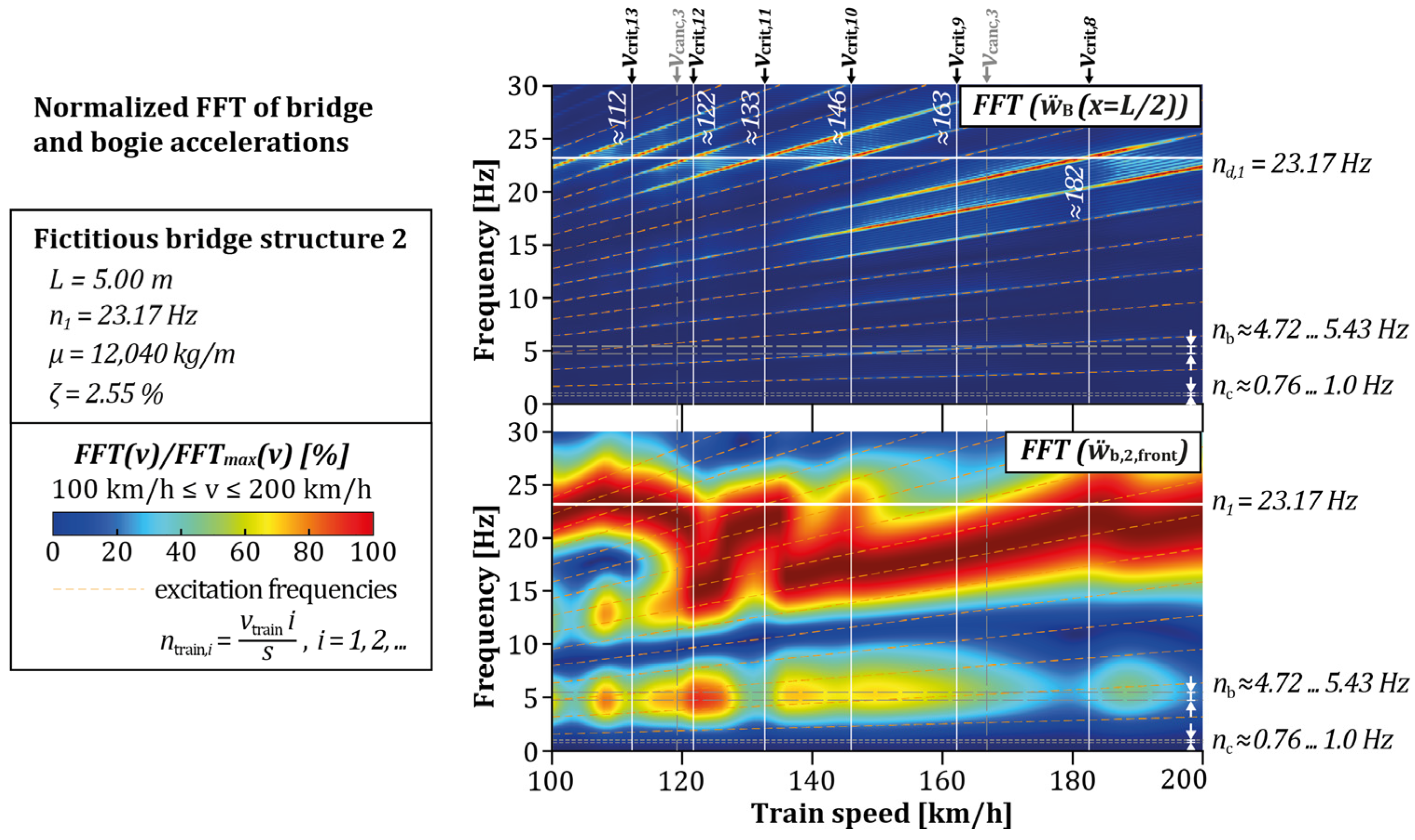
3.2. Analyses of Considered Steel Bridge in Frequency and Train Speed Domain

A fast Fourier transform (FFT) analysis of the main acceleration results is performed for each calculated train speed step. Figure 4 depicts the results obtained with the FFT analysis of the calculated acceleration results in the frequency domain for the considered steel bridge at mid-span and at the quarter points. The diagram on the left illustrates the total considered frequency range from 0 to 50 Hz, and the diagram on the right shows the frequency range from 0 to 10 Hz in more detail. It should be noted that the amplitudes in the FFT illustrations in Figure 4 and further do not directly correspond to the calculated amplitudes in the time domain, which result from the superposition of all frequency proportions.

The bridge’s resonance frequency n_d,1—the measured first bending mode of the considered bridge, see Table 1 and Section 4.2, is marked in Figure 4 at 4.52 Hz, as well as the range of natural frequencies of the bogie frames n_b and car bodies n_c, estimated for each train coach with the bogie frame mass m_b, car body mass m_c, and primary and secondary suspension stiffnesses k_p and k_s according to Equations (9) and (10), as given in ref. [53]:

$$n_{\mathrm{b}}=\frac{1}{2\pi }\sqrt{\frac{2 k_{\mathrm{p}}}{m_{\mathrm{b}}}}$$

(9)

for the bogie frames, and

$$n_{\mathrm{c}}=\frac{1}{2\pi }\sqrt{\frac{2 k_{\mathrm{s}}}{m_{\mathrm{c}}}}$$

(10)

for the car bodies. The dashed orange lines denote the excitation frequencies n_train,i resulting from the regularly spaced axle loads. The primary excitation is caused by the superimposed action of both wheels of one Jacobs bogie in the distance of s = 17.5 m to the next bogie. The resulting excitation frequencies can be calculated as follows:

$$n_{\mathrm{t}\mathrm{r}\mathrm{a}\mathrm{i}\mathrm{n},i}=\frac{v · i}{s} , i=1, 2,\dots$$

(11)

Figure 4 shows that all relevant frequency shares of the structural accelerations are caused by the excitation frequencies calculated with i = 1 to i = 8 and calculated with i = 18 to i = 21, according to Equation (11). With this, the frequency which is closest to the first bending frequency n₁ (≈ n_d,1) of the considered steel bridge causes the most prominent peak, illustrating the proximity of the examined train speed of v = 135 km/h to the bridge structures resonance speed v_crit,2 = 17.5 m · 4.52 Hz/2 = 39.55 m/s = 142.4 km/h according to Equation (5). Also, the frequency shares close to the second and third natural frequencies n_d,2 (≈ n_train,8) and n_d,3 (≈ n_train,19) are slightly higher than those of the adjacent excitation frequencies.

Furthermore, the contribution of the train masses in the system of equations of the dynamic multi-body system of the bridge structure and crossing train increases the modal masses of the bridge. This leads to a slightly lower resulting resonance frequency of the bridge structure if the train is located on the bridge compared to the unloaded bridge (e.g., described in ref. [54]). Since the FFT analysis of the bridge vibrations only included the period during the train passage and not the free decay process, the results show mainly frequency shares due to the external excitation frequencies, making it challenging to identify the bridge structure’s natural frequency. Generally, the more pronounced the acceleration peak close to n₁ becomes, the closer the excitation frequency is to the natural frequency of the bridge structure. If excitation frequencies and natural frequencies of the bridge structure differ more than in the example shown here, further analysis methods, for instance, a magnitude-squared coherence analysis of the output signal (the structural acceleration) and the input signal (the external excitation by the trains axle loads) can help to identify the natural frequency reliably from the calculation results (for example, described in ref. [55]).

Figure 5 shows the FFT results (limited from 0 to 10 Hz) obtained for the acceleration results at v = 135 km/h of the three selected bogie frames mentioned above (Figure 5a), and the adjacent car bodies, their front and rear end, respectively (Figure 5b).

It can be observed that the bogie frame vibrations feature a large frequency proportion in proximity to n_1, while the majority of frequency shares of the car bodies lie significantly below the resonance frequency of the bridge. The influence of the excitation frequencies appears to be smaller than in the case of the bridge accelerations, whereas there is a discernible influence of the natural frequency ranges of the car bodies at approximately n_c = 0.76 to 1.0 Hz and the bogie frames at n_b = 4.7 to 5.4 Hz on the acceleration shares of both train components.

The investigations of the calculated train-induced acceleration results of the considered bridge structure and selected bogie frames and car bodies of the train shown in Figure 4 and Figure 5 are subsequently carried out for all calculated train-speed steps. These FFT analysis results are exemplarily displayed in Figure 6 for the accelerations ẅ_b,2,front, the vertical vibrations at the front of the bogie b2 which enters the bridge structure analogous to the executed in situ measurements (see Section 4.3) second to last, as a three-dimensional illustration for the entire range of considered train speeds Δv₁ = 60 km/h … 420 km/h, cropped to a frequency range of 0 Hz ≤ n ≤ 10 Hz. The illustrations in Figure 5a correspond to one selected profile of FFT results at v = 135 km/h, as also shown in Figure 6b.

Both subfigures of Figure 7 illustrate the same results in the train speed/frequency plane, whereby the colors representing the acceleration amplitudes are scaled to the maximum result for the considered speed ranges Δv₁ (Figure 7a), and a more detailed investigation in Δv₂ = 100 km/h … 200 km/h respectively (Figure 7b). Again, the natural frequencies of the considered bridge n₁, the bogie frames n_b, and the car bodies n_c are marked in Figure 6b and Figure 7, as well as the characteristic resonance speeds v_crit,i, at which the excitation speed of the regularly spaced axle loads with a spacing of s = 17.5 m (defined as car length, see Figure 2) equals n₁, and the primary cancellation speeds v_canc,i, at which bridge vibrations induced by crossing loads can be canceled out, according to [52] and Equation (6).

The most prominent peaks in Figure 6a and Figure 7 emerge close to critical speeds v_crit,1 at 277 km/h (≈97% v_crit,1) and v_crit,2 at 138 km/h (≈97% v_crit,2), where, as described above, the slight undercutting of the critical speeds can be explained by the increase in the modal mass of the bridge due to the consideration of the unsprung wheelset masses of the multi-body model of the train. While the prominent peak at 277 km/h is associated with frequency shares closer to the bogie frames’ natural frequencies n_b, the second highest peak at 138 km/h appears, as seen in Figure 6, very close to the bridge structure’s first bending frequency, n₁.

Following the same principle as in Figure 6 and Figure 7, Figure 8 displays the FFT results of one adjacent car body end (ẅ_c,2,front) and the bridge vibrations at midspan (ẅ_B(x = L/2)).

Again, both the bridge structure and the examined car body experience their most prominent acceleration peak slightly below v_crit,1 at 276 or 277 km/h (≈ 97% v_crit,1). In the case of the bridge structure (Figure 8c), this peak occurs again close to the first bending frequency, n₁. Furthermore, the bridge’s resonance frequency is also recognizable in the numerically obtained calculation results of bridge accelerations in the cropped train speed range Δv₂ at again 138 km/h (≈ 97% v_crit,2), see Figure 8d, similar to the bogie frame accelerations, see Figure 7b. The car bodies’ FFT results illustrated in Figure 8a,b, however, appear to be influenced by the bridge structure’s natural frequency, particularly very close to the critical speeds v_crit,1 and v_crit,2, but are generally at significantly lower frequencies between 0 and 4 Hz, while they also scatter stronger than the results of the bridge structure and bogie frames.

Figure 9 further illustrates the close relationship between the FFT results of the bridge structure’s and the bogie frame’s accelerations. It features the planar illustration of the FFT results of both, but they are, unlike in Figure 7 and Figure 8, normalized to the maximum results at each train speed step. Additionally, the speed-dependent excitation speeds are marked with orange dashed lines according to Equation (11) and i = 1, 2, …, 6.

The illustrations indicate that there is, in principle, very similar behavior of both frequency components, i.e., at the same crossing speeds of the train, similar frequency components dominate in the vibration response of the bridge structure or the regarded bogie frame. However, these are strongly dependent on the excitation frequency and tend to agree unambiguously with the structure’s natural frequency only in the resonance case. In the case of both the bridge structure and the bogie frame, the frequency components due to the excitation frequencies that are not very close to the natural frequency of the structure n₁ are much less pronounced between approximately 120 and 155 km/h—between the two cancellation speeds v_canc,3 and v_canc,4 and in the vicinity of the critical resonance speed v_crit,2—than in the rest of the speed range considered.

In the case of the bogie frame accelerations, the respective maximum acceleration peaks in the frequency range appear as broader red or orange areas in the planar representation of Figure 8 and are, thus, less prominent than in the case of the bridge structure. In addition, a significant proportion of the velocity range also shows pronounced frequency components at 0 to 1.5 Hz, which are close to the natural frequency of the car bodies.

3.3. Comparison with Additional Considered Fictitious Bridge Structures

The existing considered bridge structure whose properties were used in setting up the bridge model features a natural frequency n_d,1 that is very close to the natural frequencies of the primary suspension stage, i.e., the bogie frames themselves. This could also explain the clear detectability of the frequency components in this frequency range in the results of the FFT analysis. In order to check whether the bridge’s natural frequency can generally be identified in the frequency components of the acceleration response of the bogie frame and to check the applicability and limits of the proposed vehicle-based iSHM method, calculations were also carried out for two further fictitious bridge structures in analogy to what was described above. Their spans L, mass distributions μ, and natural frequencies n₁ are in the range of the limit values for realistic combinations of structural properties determined based on existing bridge structures and can be seen in Table 2.

Analogous to Figure 9, the results of the FFT analysis of the train-induced acceleration responses of the bridge structure and the bogie frame, normalized to the respective maximum of a velocity step, are shown in Figure 10 and Figure 11 for these two structures, with the ordinate limited to a frequency of 30 Hz in both plots. The respective computed natural frequencies n₁ are plotted at 11.51 Hz in Figure 10 and 23.17 Hz in Figure 11, respectively, as well as the respective computed critical resonance train speeds v_crit,i and cancellation speeds v_canc,i.

Figure 10 and Figure 11 indicate that the higher the first bending frequency n₁ of the investigated structure, the more critical resonance and cancellation speeds lie in the considered train speed range. For both structures and the entire speed range, the excitation frequencies n_train,i again strongly dominate the frequency components of the acceleration response of the structure itself, which is clearly recognizable in the speed-dependent FFT results in the top illustrations. This is especially true when they coincide with the first bending frequency of the structure, i.e., in particular, at the intersections of the orange dashed lines denoting the excitation frequencies and the white horizontal line representing the computed first bending frequency of the structure (but without taking into account the slight increase in the modal masses of the bridge due to the wheelset masses of the multi-body model of the train).

In addition, the natural frequencies of the considered fictitious bridge structures can also be clearly seen in the bottom diagram of Figure 10 and Figure 11, showing the FFT results of the accelerations of bogie frame b2 during the bridge crossing event. In the case of the fictitious bridge no. 1 with a first bending frequency of n₁ = 11.51 Hz, this is mainly the case in the range from v_crit,5 to v_crit,7, while the natural frequency of the bogie frames themselves also account for more significant portions of the acceleration responses. The natural frequency of the bogie frame is also clearly pronounced in the results of the second fictitious bridge no. 2. Here, particularly at the lower train speeds, larger shares of the acceleration responses also occur in the vicinity of the first bending frequency of the bridge structure at 23.17 Hz. However, there is a substantial overlap with the excitation frequencies, and, as a result, a wide dispersion of the frequencies that make up the maximum acceleration peak is discernible, which makes it challenging to identify the bridge’s natural frequency at some speeds clearly.

4. Dynamic Measurements of the Railway Bridge and Crossing Train

4.1. Description of Steel Bridge Selected for In Situ Measurements

The railway bridge selected for in situ measurement and proof of the applicability of the proposed vehicle-based iSHM method is a single-track steel deck bridge with a ballast superstructure and a span length of 33.3 m. The two longitudinal main girders are connected through an orthotropic steel deck plate, which represents the roadway plate and supports the ballast bed (see Figure 12). A steel cantilever construction is fastened to the outer girder and serves to support the lateral walkway. The bridge is located on a railroad track with a maximum allowable train speed of 200 km/h. The relevant bridge properties are already listed in Table 1.

It is noted that two identical single-track bridges are erected in parallel positions to each other and that they are separated from each other via a longitudinal joint, i.e., coupled forced vibrations do not occur during the train crossing event. One bridge is used for the Vienna driving direction, and the second for the Salzburg driving direction. The dynamic bridge and train crossing measurements were executed at the bridge with the Salzburg driving direction.

4.2. Dynamic Measurements of Selected Steel Bridge

Forced vibration tests were carried out to identify the natural frequencies, corresponding mode shapes, and damping ratios of the considered railway bridge. Therefore, two electrodynamic long-stroke shakers, SH1 and SH2, were fastened at the center of the longitudinal main girders beneath the bridge using a stiff hanging construction (see Figure 13).

The installed long-stroke shakers have a static mass of around 70 kg and an additional vertical moving mass of 30.6 kg each. Depending on the excitation frequency, excitation force amplitudes up to 440 N for each of the electrodynamic shakers can be applied to the bridge structure. A closed-loop control system enables a constant force amplitude over the entire excitation frequency range of interest, and it is possible to synchronize and operate with several shakers at the same time. Additionally, the asynchronous operation of the two installed long-stroke shakers allows the identification of torsional vibration modes of the considered bridge. Using these shakers ensures the ability to reproduce the measurement results, and a high accuracy is achievable. For this specific measurement, the shakers were fastened hanging on the bottom flange of the main girders. In order to measure the vibration response of the harmonic force-excited bridge, several accelerometers were installed in different locations of the main girders. The sensor and shaker positions are shown in Figure 14.

Figure 15 illustrates the measured amplitude-frequency response function, evaluated from the executed continuous frequency sweep from 2 to 12 Hz, with a sweeping speed of 2 Hz/min and a constant excitation force amplitude of F₀ = 428 N of the two installed synchronized shakers. Three peaks can be detected in the gained frequency spectrum at 3.85 Hz, 4.52 Hz, and 5.51 Hz. The highest peak with a frequency of n_d,1 = 4.52 Hz corresponds to the first bending mode of the bridge where the two main girders exhibit a vibration response in phase with more or less the same size of dynamic displacement, and it is evaluated as most critical regarding train-induced resonance vibrations. Hence, the later applied vehicle-based iSHM method focuses on identifying this most relevant bridge’s natural frequency.

The two detected additional frequencies at 3.85 Hz and 5.51 Hz correspond to local vibration modes of the longitudinal main girders 1 and 2; see Figure 14. The outer main girder 1 supports the cantilever steel construction, and hence, its frequency and vibration amplitude are lower than the frequency of the inner main girder 2 (cf. Figure 15). This interesting finding of two local vibration modes is a bridge-specific characteristic that must be considered during the measurement data analysis and interpretation.

The damping ratio ζ of the bridge’s most relevant first bending mode is determined by applying the half-power bandwidth method to the acceleration amplitude frequency response function in Figure 15 and results in ζ = 1.88% as a mean value out of five repeatedly conducted measurements with the same test setup. Thereby, the standard deviation of the measured damping ratios is determined by σ = 0.012%, which is very small and confirms the advantage of the applied forced vibration testing method.

In addition to the synchronous sweep, an asynchronous sweep was executed with a sweeping speed of 2 Hz/min and a constant excitation force amplitude of F₀ = 214 N per shaker. In the case of the asynchronous sweep, the two shakers operate with a phase shift of 180°, and torsional modes of the bridge are expected to be excited dominantly. The gained amplitude-frequency response function, evaluated from the executed continuous frequency sweep with two shakers in an asynchronous operating mode, is shown in Figure 16. A plausible result emerges, namely that the bridge´s most relevant first bending frequency, n_d,1 = 4.52 Hz, is not excited because of the asynchronous operating mode of the two installed shakers. However, the two from Figure 14 already identified local vibrating frequencies of the main girders at 3.85 Hz and 5.51 Hz are again clearly visible, and a third local frequency can also be identified at 3.65 Hz. However, the analysis of recorded data of train crossing events in Section 4.3 shows that the bridge’s first bending mode, n_d,1 = 4.52 Hz (measured value), is dominantly excited through the crossing train and, therefore, it is selected for application of the vehicle-based iSHM method presented here.

4.3. Dynamic Measurements of Crossing Train

In order to measure the forced vibration responses of the traveling train during the bridge crossing event, a set of 27 accelerometers were installed at different locations of the train (see Figure 17). The sampling rate was chosen at 2400 Hz, and the sensor signals were permanently recorded during train traveling. Before carrying out the measurements on the train, research was undertaken on the appropriate acceleration sensors available on the market. Due to the high acceleration amplitudes expected on the wheelsets and bogies during train traveling, the requirement of a sufficient high measuring range was defined as the first important parameter. Further requirements for the applied sensors were a high resolution of the measurement signals, high sensitivity, an optimal working frequency range, a resonant frequency of the sensor much higher than the frequency range of interest, and a low non-linearity. Based on the defined requirements, the accelerometers of the Integrated Circuit Piezoelectric (ICP) type were evaluated as most appropriate for measuring the train vibrations, and the specifications of the selected sensors are:

Measurement range	±50 g peak
Frequency range (±5%)	1 to 4000 Hz
Frequency range (±10%)	0.7 to 7000 Hz
Frequency range (±3 dB)	0.35 to 12,000 Hz
Resonant frequency	≥22 kHz
Broadband resolution	0.0005 g rms
Non-Linearity	≤1%

The total length of the considered train is 202 m, and it consists of 11 coaches (c1 to c11) interconnected through 12 Jacobs bogies (b1 to b12). The bogies b2 to b11 are regularly spaced at s = 17.5 m, and bogies b1 and b12 are at a distance of 16.7 m from the corresponding adjacent bogies. Three bogies of the train (b2, b6, and b11) were selected for instrumentation of uniaxial accelerometers and their installation positions are as follows (exemplarily described for bogie b2): accelerometers a333 and a334 installed at the car bodies; accelerometers a213, a223, and a224 installed at the bogie frames; accelerometers a113, a114, a123, and a124 installed at the wheelsets.

The train test runs were carried out with four different train speeds (135 km/h, 150 km/h, 160 km/h, and 165 km/h) in both driving directions (Vienna and Salzburg). Every test run was repeated two times in every driving direction, i.e., the total measured train runs were 16. Because only the steel deck bridge with the track in the Salzburg driving direction was dynamically measured by application of forced vibration testing (cf. Section 4.2), the train vibration responses during bridge crossing were just analyzed for the test runs with the Salzburg driving direction. Even though the vibration responses of the crossing vehicle were measured for all considered train speeds and at the location of every installed accelerometer (see Figure 17), a detailed data analysis was carried out for the most relevant (lowest) train speed at 135 km/h (cf. Section 3.2 and note that the resonance speed v_crit,2 = 142.4 km/h is close to the analyzed train speed) and considering the accelerometers installed to the bogie frame b2 and car body c1. These sensors were selected for the evaluation of recorded data in accordance with the conducted numerical simulations to compare the results (see Figure 6 in Section 3.2). Additionally, the analyses of the measurement data identified that the most reliable identification of the bridge´s first bending frequency is achieved considering the vibration responses of bogie b2 that enters the bridge as second to last. However, it is planned to analyze the total recorded data within a further research project to investigate the application of further data evaluation methods in the time and frequency domain. It should be noted that the sensors installed on the considered steel bridge remained installed according to the positions shown in Figure 14; thus, both the vehicle and bridge vibration responses were measured during the train crossing events and analyzed in this section.

Figure 18a illustrates the relevant low-pass filtered time-history section of the measured forced vibration response of bogie frame b2 for accelerometer a213 during the train crossing event. Figure 18b shows the corresponding frequency response function calculated by FFT. Therefore, the filter cut-off frequency was chosen as 10 Hz. In addition, Figure 18c,d shows the measured vibration response of the car body c1 for accelerometers a333 and the corresponding FFT result. In this measurement, the train run was executed with the Salzburg driving direction at 135 km/h (=37.5 m/s), and hence, the considered bogie b2 arrived as the second to last bogie on the steel bridge (see Figure 17).

In relation to the bridge span length of 33.3 m, the duration of the bogie crossing at 135 km/h is just around 1 s, and hence, selecting the relevant time section for calculating the corresponding frequency spectra is essential. It is seen from the FFT result of the vibration response of the bogie frame b2 (Figure 18b) that the bridge’s natural frequency, which was already determined by the forced vibrations tests (cf. measured value n_d,1 = 4.52 Hz, see Section 4.2)—can be identified at n_d,1,TI = 4.38 Hz and this train-identified frequency agrees quite good with the result of the dynamic bridge measurements. The slight difference of around 3% between the in situ measured and train-identified first bending frequency is attributed to the vehicle–bridge-interaction effect, in particular, the unsprung train-mass-induced frequency shift (cf. Section 3.2).

The additional peaks that are visible in the frequency response function of Figure 18b correspond most likely to excited resonance frequencies of the bogie, which obviously also occur in the frequency spectra (cf. calculated bogie frequencies in Section 3.2). The frequency response function given in Figure 18d, calculated from the vibration response of the car body c1, does not allow the identification of the bridge’s natural frequency. It is assumed that the dominant visible frequency of 1.34 Hz corresponds to the low vertical vibration mode of the car body, which is also evident in a similar form (at 0.9 to 1.9 Hz) in the analysis of the numerically derived vibration response of the car bodies (see Figure 5 in Section 3.2).

To prove that the selected train-identified frequency peak of n_d,1,TI = 4.38 Hz in Figure 18b corresponds to the first bending frequency of the considered steel bridge, the measured acceleration response of the considered steel bridge during train crossing at 135 km/h is illustrated in Figure 19a for sensor A2 in the time-domain. In addition, Figure 19b shows the FFT result of the time decay function after the train has completely left the bridge. It is noted that the displayed acceleration signal of the sensor A2 has been low-pass filtered with a cut-off frequency of 20 Hz.

It is seen from the FFT result of the time decay function in Figure 19b that the highest frequency peak occurs at 4.38 Hz, which is close to the bridge’s first bending frequency n_d,1 = 4.52 Hz determined via forced vibration tests (see Figure 15). This indicates that the first bending mode of the bridge is dominantly excited during the train crossing event. The determined frequency of the time-decay function agrees very well with the train-identified frequency of n_d,1,TI = 4.38 Hz. Hence, the train-identified frequency n_d,1,TI can be assigned to the first bending frequency of the bridge.

5. Conclusions

The vehicle-based iSHM method was applied to determine the natural frequencies of railway bridges by measurements of the train vibration responses during the bridge crossing event only. Numerical train crossing simulations were carried out for an existing steel deck bridge as well as two further fictitious railway bridges, considering a multi-body model for the traveling train and a simply-supported single-span Euler–Bernoulli beam.

In order to validate the results of the numerical simulations, in situ tests were executed at the existing steel deck bridge, and both the steel bridge and the traveling train were instrumented with accelerometers. At first, forced vibration tests were performed to determine the natural frequencies and damping ratio of the steel bridge. Second, the vibration responses of the train and the bridge were measured during the train crossing events. It could be shown that in the numerical simulations as well as in the in situ measurements, the FFT-transformed vibration responses of the bogie frame b2 during train crossing allow the most reliable extraction of the first bending frequency of the considered railway bridge.

In summary, the following outcomes of the research are drawn:

• The executed analyses—shown here only for a particular bogie frame of the considered train, for a particular traveling direction, and three exemplary realistic railway bridge structures—indicate a strong similarity in the dynamic behavior of the bridge and the bogie frames during train crossing. This is particularly evident in the frequency domain, although identifying the bridge’s natural frequency is only possible when analyzing a wider range of speeds, including at least one resonant speed;
• At crossing speeds of the trains, which are not very close to resonance speeds or where a cancellation speed is close, the frequency components resulting from the excitation frequencies dominate the acceleration response of the bridge structure and bogie frame. The same applies to cases where the bogie frames, for which the natural frequency of the primary stage is—as in the case of the existing steel deck bridge—also in the vicinity of the first bending frequency;
• The conducted forced vibration tests of the existing steel deck bridge and, in particular, the bridge´s natural frequencies and damping ratio determined turned out to be an important basis for the reliable identification of the bridge´s first bending mode by application of vehicle-based iSHM method;
• In situ measurements of both the train and bridge vibration responses were performed during the train crossing events, and thus, it could be shown that the first bending frequency of the bridge n_d,1 = 4.52 Hz (determined by forced vibration testing), was dominantly excited through the crossing train at 135 km/h;
• The first bending frequency of the bridge was clearly determined by the application of the vehicle-based iSHM method, considering the frequency response function of bogie frame vibrations during the train crossing event at 135 km/h. The train-identified bridge´s bending frequency was identified with n_d,1,TI = 4.38 Hz, which is in accordance with the numerical results and around 3% smaller than the value determined by forced vibration testing.

Finally, it is concluded that the application of the vehicle-based iSHM method provides a promising tool for identifying the dynamic characteristics of railway bridges by only measuring the vibration responses of the crossing train. In particular, potentially identifying changes in the natural frequencies of the structure, which can indicate possible damage to the structure during regular railway operations, is a promising application possibility for predictive maintenance to be explored with further development of the method. However, challenges were detected regarding the reliable identification of the bridge´s natural frequencies from the bogie frame vibration responses only, without having the results of the bridge´s frequencies from performed in situ measurements. The processing of the mentioned challenges and a more detailed analysis of the recorded data by considering all installed sensors and applying different evaluation methods will be performed in future research.

References

- Reiterer, M.; Firus, A. Dynamische Analyse der Zugüberfahrt bei Eisenbahnbrücken unter Berücksichtigung von nichtlinearen Effekten. Beton-Und Stahlbetonbau 2021, 117, 90–98. [Google Scholar] [CrossRef]
- EN 1990:2002/A1:2005/AC:2010; Eurocode—Basis of Structural Design. CEN European Committee for Standardization: Brussels, Belgium, 2021.
- RW 08.01.04; Dynamische Berechnung von Eisenbahnbrücken, Anhang 1: Zugdefinitionen. ÖBB-Infrastruktur AG: Vienna, Austria, 2022.
- Allahvirdizadeh, R.; Andersson, A.; Karoumi, R. Improved dynamic design method of ballasted high-speed railway bridges using surrogate-assisted reliability-based design optimization of dependent variables. Reliab. Eng. Syst. Saf. 2023, 238, 109406. [Google Scholar] [CrossRef]
- Reiterer, M.; Firus, A.; Vorwagner, A.; Lombaert, G.; Schneider, J.; Kohl, A.M. Railway bridge dynamics: Development of a new high-speed train load model for dynamic analyses of train crossing. In Proceedings of the IABSE Congress Ghent 2021—Structural Engineering for Future Societal Needs, Ghent, Belgium, 22–24 September 2021. [Google Scholar] [CrossRef]
- Farrat, C.R.; James, G.H., III. System identification from ambient vibration measurements on a bridge. J. Sound Vib. 1997, 205, 1–18. [Google Scholar] [CrossRef]
- Reiterer, M. Experimentelle und numerische Untersuchung einer bestehenden Eisenbahnbrücke bei Zugüberfahrt. Bautechnik 2020, 97, 473–489. [Google Scholar] [CrossRef]
- Huang, C.S.; Yang, Y.B.; Lu, L.Y.; Chen, C.H. Dynamic testing and system identification of a multi-span highway bridge. Earthq. Eng. Struct. Dyn. 1999, 28, 857–878. [Google Scholar] [CrossRef]
- Reiterer, M.; Lachinger, S.; Fink, J.; Bruschetini-Ambro, S.-Z. Ermittlung der dynamischen Kennwerte von Eisenbahnbrücken unter Anwendung von unterschiedlichen Schwingungsanregungsmethoden. Bauingenieur 2017, 92, 2–13. (In German) [Google Scholar]
- Yang, Y.B.; Lin, C.W.; Yau, J.D. Extracting bridge frequencies from the dynamic response of a passing vehicle. J. Sound Vib. 2004, 272, 471–493. [Google Scholar] [CrossRef]
- Lin, C.W.; Yang, Y.B. Use of a passing vehicle to scan the fundamental bridge frequencies: An experimental verification. Eng. Struct. 2005, 27, 1865–1878. [Google Scholar] [CrossRef]
- Tan, C.; Elhattab, A.; Uddin, N. “Drive-by” bridge frequency-based monitoring utilizing wavelet transform. J. Civ. Struct. Health Monit. 2017, 7, 615–625. [Google Scholar] [CrossRef]
- Yang, Y.B.; Zhang, B.; Chen, Y.A.; Qian, Y.; Wu, Y.T. Bridge damping identification by vehicle scanning method. Eng. Struct. 2019, 183, 637–645. [Google Scholar] [CrossRef]
- Yang, Y.; Li, Z.; Wang, Z.; Shi, K.; Xu, H.; Qiu, F.; Zhu, J. A novel frequency-free movable test vehicle for retrieving modal parameters of bridges: Theory and experiment. Mech. Syst. Signal Process. 2022, 170, 108854. [Google Scholar] [CrossRef]
- Urushadze, S.; Yau, J.-D.; Yang, Y.-B.; Bayer, J. Theoretical and Experimental Verifications of Bridge Frequency Using Indirect Method. In Dynamics of Civil Structures; Springer: Berlin/Heidelberg, Germany, 2020; Volume 2, pp. 153–158. [Google Scholar]
- Tan, C.; Zhao, H.; OBrien, E.J.; Uddin, N.; Fitzgerald, P.C.; McGetrick, P.J.; Kim, C.-W. Extracting mode shapes from drive-by measurements to detect global and local damage in bridges. Struct. Infrastruct. Eng. 2021, 17, 1582–1596. [Google Scholar] [CrossRef]
- Tan, C.; Elhattab, A.; Uddin, N. Wavelet-Entropy Approach for Detection of Bridge Damages Using Direct and Indirect Bridge Records. J. Infrastruct. Syst. 2020, 26, 04020037. [Google Scholar] [CrossRef]
- Tan, C.; Uddin, N. Hilbert transform based approach to improve extraction of “drive-by” bridge frequency. Smart Struct. Syst. 2020, 25, 265–277. [Google Scholar] [CrossRef]
- McGetrick, P.J.; Gonzalez, A.; Obrien, E.J. Theoretical investigation of the use of a moving vehicle to identify bridge dynamic parameters. Insight 2009, 51, 433–438. [Google Scholar] [CrossRef]
- Siringoringo, D.M.; Fujino, Y. Estimating Bridge Fundamental Frequency from Vibration Response of Instrumented Passing Vehicle: Analytical and Experimental Study. Adv. Struct. Eng. 2012, 15, 417–433. [Google Scholar] [CrossRef]
- Kong, X.; Cai, C.S.; Kong, B. Numerically Extracting Bridge Modal Properties from Dynamic Responses of Moving Vehicles. J. Eng. Mech. 2016, 142, 04016025. [Google Scholar] [CrossRef]
- Elhattab, A.; Uddin, N.; Obrien, E. Drive-By Bridge Frequency Identification under Operational Roadway Speeds Employing Frequency Independent Underdamped Pinning Stochastic Resonance (FI-UPSR). Sensors 2018, 18, 4207. [Google Scholar] [CrossRef]
- Mei, Q.P.; Gul, M.; Boay, M. Indirect health monitoring of bridges using Mel-frequency cepstral coefficients and principal component analysis. Mech. Syst. Signal Process. 2019, 119, 523–546. [Google Scholar] [CrossRef]
- Gonzalez, A.; OBrien, E.J.; McGetrick, P.J. Identification of damping in a bridge using a moving instrumented vehicle. J. Sound Vib. 2012, 331, 4115–4131. [Google Scholar] [CrossRef]
- Keenahan, J.; Obrien, E.J.; McGetrick, P.J.; Gonzalez, A. The use of a dynamic truck–trailer drive-by system to monitor bridge damping. Struct. Health Monit. Int. J. 2013, 13, 143–157. [Google Scholar] [CrossRef]
- Tan, C.J.; Uddin, N.; OBrien, E.J.; McGetrick, P.J.; Kim, C.W. Extraction of Bridge Modal Parameters Using Passing Vehicle Response. J. Bridge Eng. 2019, 24, 04019087. [Google Scholar] [CrossRef]
- Malekjafarian, A.; Brien, E.J. Identification of bridge mode shapes using Short Time Frequency Domain Decomposition of the responses measured in a passing vehicle. Eng. Struct. 2014, 81, 386–397. [Google Scholar] [CrossRef]
- Yang, Y.B.; Li, Y.C.; Chang, K.C. Constructing the mode shapes of a bridge from a passing vehicle: A theoretical study. Smart Struct. Syst. 2014, 13, 797–819. [Google Scholar] [CrossRef]
- Oshima, Y.; Yamamoto, K.; Sugiura, K. Damage assessment of a bridge based on mode shapes estimated by responses of passing vehicles. Smart Struct. Syst. 2014, 13, 731–753. [Google Scholar] [CrossRef]
- Malekjafarian, A.; OBrien, E.J. On the use of a passing vehicle for the estimation of bridge mode shapes. J. Sound Vib. 2017, 397, 77–91. [Google Scholar] [CrossRef]
- Marulanda, J.; Caicedo, J.M.; Thomson, P. Mode shapes identification under harmonic excitation using mobile sensors. Ing. Compet. 2017, 19, 140–145. [Google Scholar]
- Zhang, Y.; Wang, L.Q.; Xiang, Z.H. Damage detection by mode shape squares extracted from a passing vehicle. J. Sound Vib. 2012, 331, 291–307. [Google Scholar] [CrossRef]
- OBrien, E.J.; Malekjafarian, A. A mode shape-based damage detection approach using laser measurement from a vehicle crossing a simply supported bridge. Struct. Control Health Monit. 2016, 23, 1273–1286. [Google Scholar] [CrossRef]
- Domaneschi, M.; Limongelli, M.P.; Martinelli, L. Vibration Based Damage Localization Using MEMS on a Suspension Bridge Model. Smart Struct. Syst. 2013, 12, 679–694. [Google Scholar] [CrossRef]
- Domaneschi, M.; Limongelli, M.P.; Martinelli, L. Multi-Site Damage Localization in a Suspension Bridge via Aftershock Monitoring. Ing. Sismica 2013, 30, 56–72. [Google Scholar]
- Domaneschi, M.; Sigurdardottir, D.; Glisic, B. Damage detection based on output-only monitoring of dynamic curvature in concrete-steel composite bridge decks. Struct. Monit. Maint. 2017, 4, 1–15. [Google Scholar] [CrossRef]
- Vospernig, M.; Reiterer, M. Evaluation of the dynamic system characteristics for single span concrete railway bridges—Determination of dynamic parameters due to measurements on two test bridges in cracked and uncracked state with variations of the dead load. Beton Und Stahlbetonbau 2020, 115, 424–437. [Google Scholar] [CrossRef]
- Zhan, J.; You, J.; Kong, X.; Zhang, N. An indirect bridge frequency identification method using dynamic responses of high-speed railway vehicles. Eng. Struct. 2021, 243, 112694. [Google Scholar] [CrossRef]
- Frýba, L.; Kadecka, S. ICE Virtual Library. Dynamics of Railway Bridges; Telford, T., Ed.; Publications Sales Department, American, Society of Civil Engineers: New York, NY, USA; London, UK, 1996. [Google Scholar]
- Sun, Y.Q.; Dhanasekar, M. A dynamic model for the vertical interaction of the rail track and wagon system. Int. J. Solids Struct. 2002, 39, 1337–1359. [Google Scholar] [CrossRef]
- Yang, Y.B.; Yau, J.D.; Wu, Y.S. Vehicle-Bridge Interaction Dynamics: With Applications to High-Speed Railways; World Scientific: River Edge, NJ, USA; London, UK, 2004. [Google Scholar]
- Lou, P. Finite element analysis for train–track–bridge interaction system. Arch. Appl. Mech. 2007, 77, 707–728. [Google Scholar] [CrossRef]
- Mähr, T.C. Theoretische und experimentelle Untersuchungen zum dynamischen Verhalten von Eisenbahnbrücken mit Schotteroberbau unter Verkehrslast. Ph.D. Thesis, TU Wien, Vienna, Austria, 2008. (In German). [Google Scholar]
- Glatz, B.; Fink, J. A redesigned approach to the additional damping method in the dynamic analysis of simply supported railway bridges. Eng. Struct. 2021, 241, 112415. (In German) [Google Scholar] [CrossRef]
- Bettinelli, L.; Stollwitzer, A.; Fink, J. Numerical Study on the Influence of Coupling Beam Modeling on Structural Accelerations during High-Speed Train Crossings. Appl. Sci. 2023, 13, 8746. [Google Scholar] [CrossRef]
- EN 1991-2:2003/AC:2010; Eurocode 1: Actions on Structures—Part 2: Traffic Loads on Bridges. CEN European Committee for Standardization: Brussels, Belgium, 2010.
- Lei, X.; Noda, N.A. Analyses of dynamic response of vehicle and track coupling system with random irregularity of track vertical profile. J. Sound Vib. 2002, 258, 147–165. [Google Scholar] [CrossRef]
- Dinh, V.N.; Du Kim, K.; Warnitchai, P. Dynamic analysis of three-dimensional bridge–high-speed train interactions using a wheel–rail contact model. Eng. Struct. 2009, 31, 3090–3106. [Google Scholar] [CrossRef]
- Cantero, D.; Arvidsson, T.; OBrien, E.; Karoumi, R. Train–track–bridge modelling and review of parameters. Struct. Infrastruct. Eng. 2016, 12, 1051–1064. [Google Scholar] [CrossRef]
- The Mathworks Inc. MATLAB 2022; The Mathworks Inc.: Natick, MA, USA, 2022. [Google Scholar]
- Shampine, L.F.; Reichelt, M.W. The MATLAB ODE Suite. SIAM J. Sci. Comput. 1997, 18, 1–22. [Google Scholar] [CrossRef]
- Xia, H.; Li, H.L.; Guo, W.W.; de Roeck, G. Vibration Resonance and Cancellation of Simply Supported Bridges under Moving Train Loads. J. Eng. Mech. 2014, 140, 04014015. [Google Scholar] [CrossRef]
- Doménech, A.; Museros, P.; Martínez-Rodrigo, M.D. Influence of the vehicle model on the prediction of the maximum bending response of simply-supported bridges under high-speed railway traffic. Eng. Struct. 2014, 72, 123–139. [Google Scholar] [CrossRef]
- Arvidsson, T.; Karoumi, R.; Pacoste, C. Statistical screening of modelling alternatives in train–bridge interaction systems. Eng. Struct. 2014, 59, 693–701. [Google Scholar] [CrossRef]
- Yan, W.J.; Feng, Z.; Ren, W.X. New insights into coherence analysis with a view towards extracting structural natural frequencies under operational conditions. Measurement 2016, 77, 187–202. [Google Scholar] [CrossRef]