The Dynamic Train–Track Interaction on a Bridge and in a Tunnel Compared with the Simultaneous Vehicle, Track and Ground Vibration Measurements on a Surface Line

Abstract

The vehicle–track interaction generates forces and consequently vibrations in the environment. The interaction has been analysed by the simultaneous measurements of vehicle, track and ground vibrations during test runs with varied train speeds. The special effects of the passage over a bridge and through a tunnel are studied and compared with the measurements on a conventional ballasted surface line. The maximum amplitudes, narrow band and one-third octave band spectra are presented for the axle-box accelerations and for the track, bridge and ground vibrations. The different frequencies and frequency bands are related to wheel out-of-roundness, track alignment errors, the sleeper passage and the wheelset–track resonance. An axle impulse component has been observed at the track, at the near-field soil and as a scattered version in the far field. Specific results can be found for the bridge track, where clearly speed-dependent bridge resonances occur due to the axle sequence of the train, and for the tunnel track where soft rail pads are responsible for a strong amplification around the wheelset–track resonance. On the other hand, the axle impulses are strongly reduced by the tunnel track, and the scattered axle impulse component is not as relevant as for the surface track. As a consequence, a strong mid-frequency amplitude reduction of the tunnel compared to the surface line has been measured for low and high train speeds by the Federal Institute of Material Research and Testing (BAM) and by other institutes.

1. Introduction

High-speed railway lines often run through tunnels and on bridges, and the train-induced ground vibrations need to be predicted. The aim of this contribution is to analyse the effects of these special track or line types from measurements, while calculations for tunnel and bridge lines have been included in the companion paper [1]. The BAM has performed simultaneous measurements of the vehicle, track and ground vibrations during test runs on the high-speed line near Würzburg where a tunnel, bridge and surface section were included [2]. This combination of vibration measurements is unique and allows new insights into the vehicle–track–soil interaction and the excitation of ground vibration. Whereas the results for the surface line have been evaluated in [3], the focus is now set on the specific behaviour of the bridge and the tunnel line.

Vibration measurements of vehicle vibration for vehicle problems are often found, see in [4], as well as track measurements for track problems, e.g., [5]. Moreover, vehicle measurements can be used for the monitoring of the track, e.g., [6], and track measurements for the monitoring of the vehicle, e.g., [7], where the vehicle–track interaction is included. Combined vibration measurements of the vehicle, track and ground as presented here are not found in the literature.

There is a wide literature about the vibrations of railway bridges, for example [8,9,10], and the amplification and cancellation of bridge resonances have been well studied [11,12]. The combination of the bridge analysis with the generated ground vibration, however, is quite rare, for example Wu and Yan [13]. Measurements of bridge vibrations and their resonances have been shown for example in Xia et al. [14] for different speeds, and in Museros et al. [15] for different bridges, but the focus is usually on regular high-speed trains and not on conventional passenger trains which are analysed in the present article. A few articles [16,17,18] combine a detailed theory with experimental results about ground vibration. Ju and Lin [16] include a parameter study about resonances of simply supported bridges, the influence of the vehicle–bridge interaction and a comparison of measured ground vibrations with the numerical results of a big finite-element model of a 21-span viaduct with a span length of 30 m. The standard Chinese high-speed bridge, which has a simply supported span length of 32 m, has been analysed in detail by Xing et al. [17] for bridge and ground vibrations. The Japanese high-speed viaduct, which consists of 24 m long frame segments of three 6 m long spans and 2 × 3 bridge piers, has been analysed theoretically and with bridge and ground vibration measurements by Takemiya and Bian [18]. More measurements near bridge lines, also for freight trains or urban trains, can be found in [19,20,21,22]. Many of these references address the strong attenuation of the ground vibrations with the distance from the bridge pier which can be attributed to the special point-load excitation for a bridge line. Some details of ground vibration measurements near bridge lines will be discussed in this contribution. The BAM measurements will be evaluated for the bridge resonances and their dependence on the axle sequence and the speed of the train.

Measurements of ground vibrations near railway tunnels have been reported in [23,24,25,26,27], where they have been used to verify numerical tunnel–soil models. In [28], some rules for the excitation of the ground vibrations have been derived from measurements at tunnel lines. It seems that the maximum amplitudes generally occur in a frequency range of 50 to 100 Hz higher than what is usually found for surface lines, but only a few measurements directly compare the vibrations from a tunnel and a surface line. In [29], the measurements at a near-surface tunnel were evaluated for a surface-to-tunnel reduction. In [30], measurements in Germany and France were reported which lead to a strong surface-to-tunnel reduction to be used for the prediction in the British Highspeed2 project. The Austrian Institute of Technology has performed a detailed measurement campaign with train and shaker excitation of a deep tunnel and a surface line [31]. All these measurements in [29,30,31] and the BAM measurements in [2,32,33] will be consistently evaluated in this contribution. Moreover, the frequency-dependent characteristics presented in this article give the missing reasons for the differences in the vibrations between tunnel and surface lines.

A unique measurement campaign has been performed by BAM (Section 2). The different measurement results for the vehicle, track and ground are described by one-third octave band spectra (Section 3). The special effects of the bridge and the tunnel line are analysed in detail by time histories and Fourier spectra (Section 4). The surface-to-tunnel reduction is evaluated for the present measurement campaign with low train speeds up to 160 km/h. The results are compared with similar measurement results for high-speed trains which have been performed by BAM and other institutes (Section 5). The measurement results are compared with theoretical results to give some explanation of the observed reductions for the tunnel and the observed amplifications for the bridge (Section 6). The significant contributions of this article (the explanation of the bridge resonance by the axle sequence spectrum and the tunnel-to-surface reduction by the scattered axle impulses) are summarized in the conclusion.

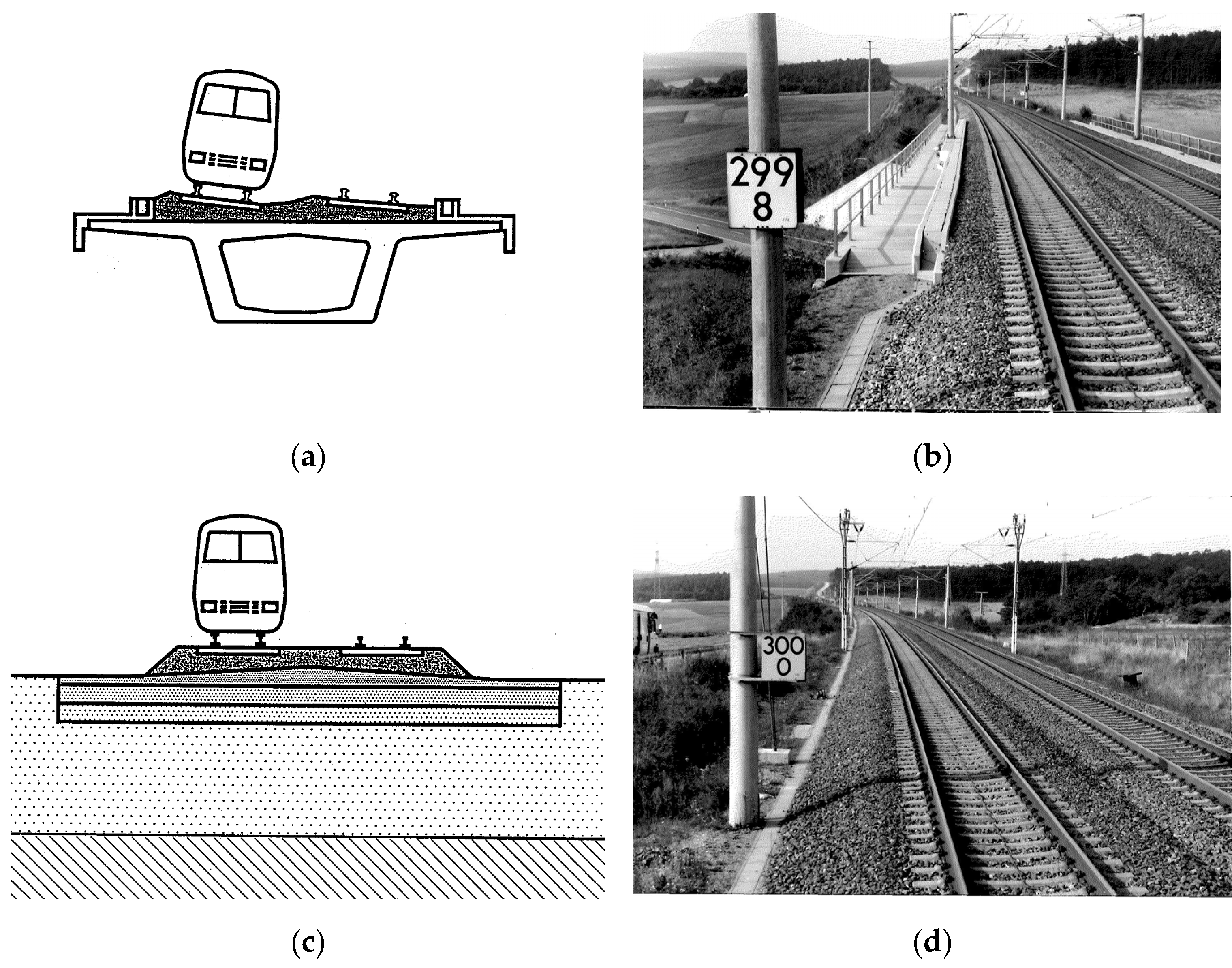
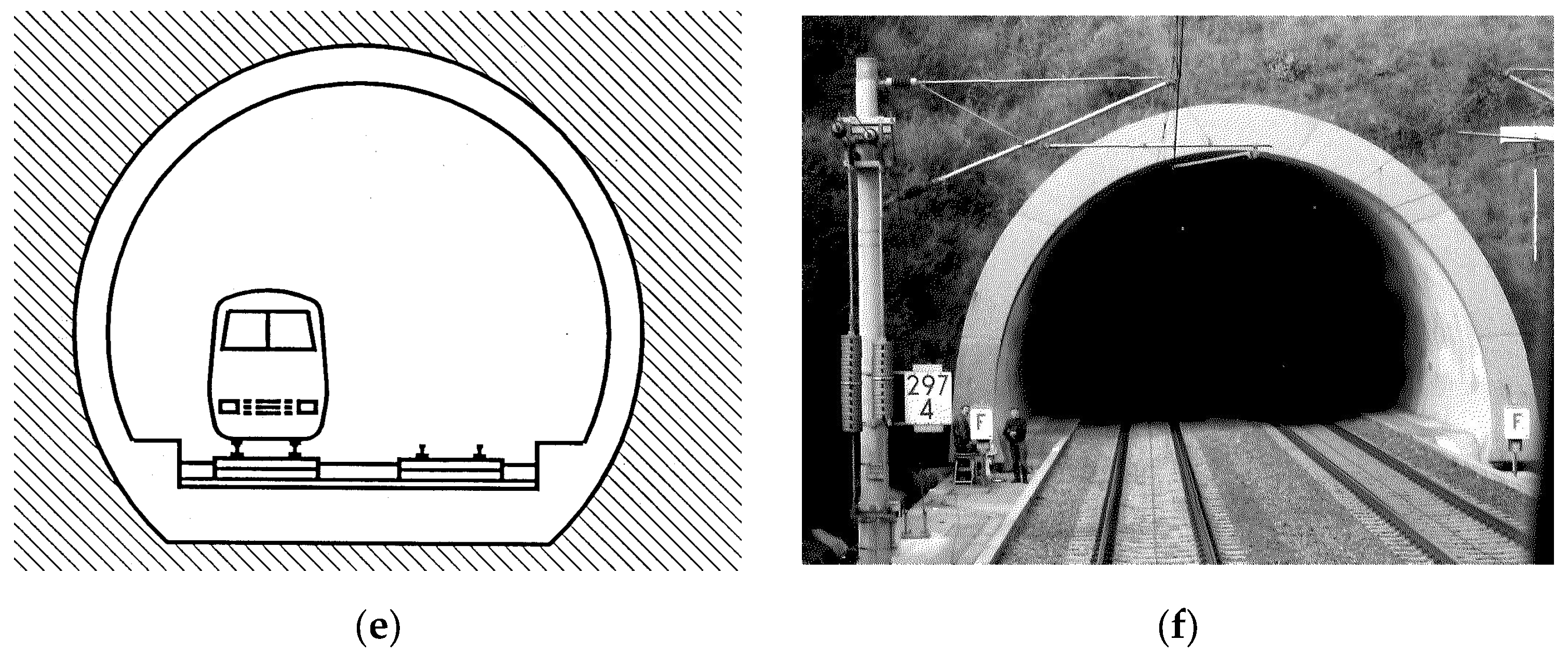
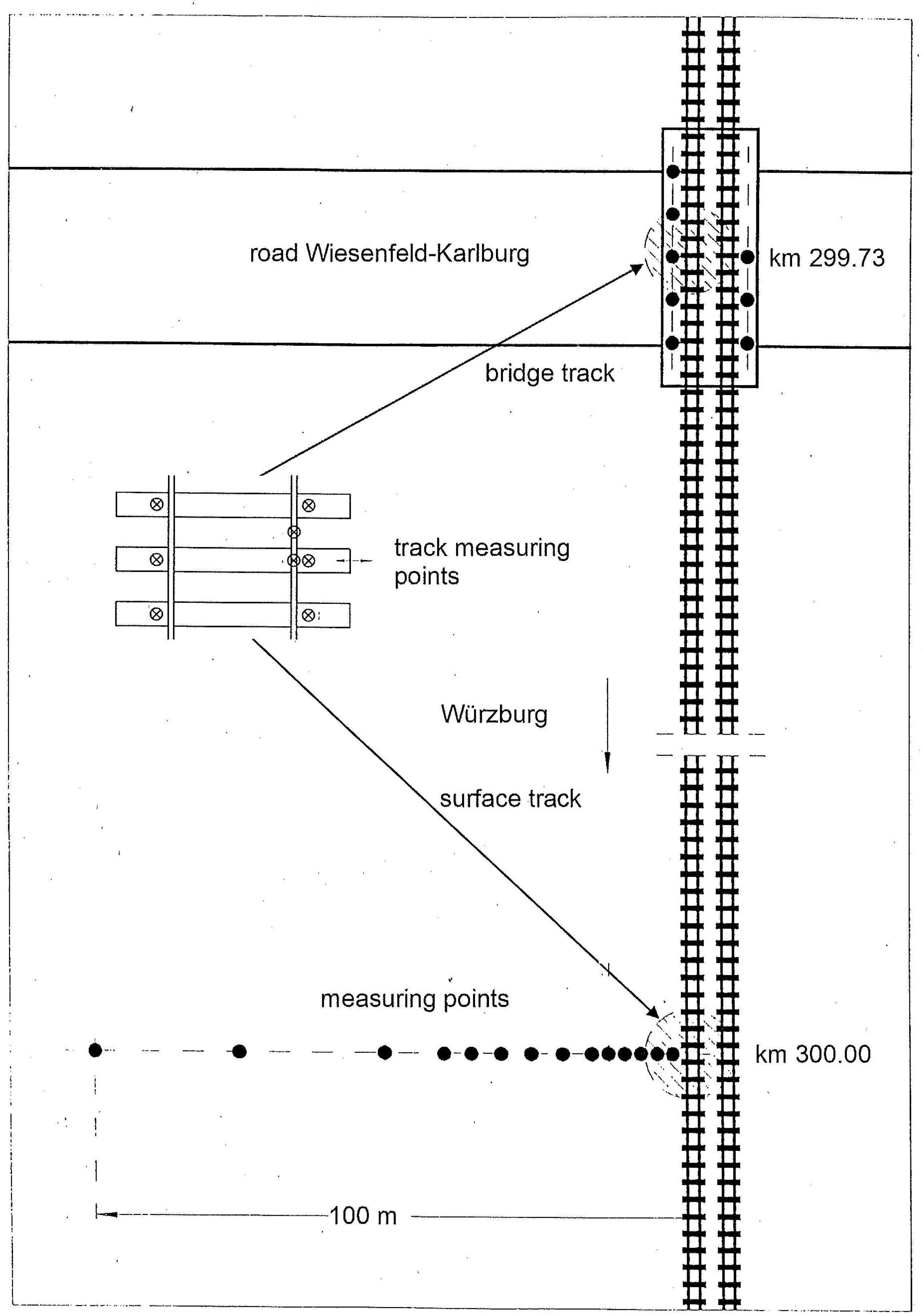
2. Measurement Campaign for the Bridge, Tunnel and Surface Lines

A unique measurement campaign has been performed by the Federal Institute of Material Research and Testing (BAM) on a 3 km long section of the German high-speed line Hannover–Würzburg [2]. Vehicle, track and ground vibrations have been measured simultaneously at a tunnel (the Mühlberg tunnel), a 45 m long box-girder concrete bridge and a conventional ballasted surface track (Figure 1) for passages of a 7-unit test train (locomotive, 5 passenger cars, locomotive) with regularly varied speeds of v_T = 63, 80, 100, 125,140 and 160 km/h. The measurement points are documented in Figure 2 and Figure 3. The ground vibrations were measured at the soil surface from 3 to 50 m (tunnel line) and from 3 to 100 m (surface line) horizontal distance from the track with geophones (active velocity transducers Geospace HS-1 with 4.5 Hz natural frequency). Geophones were also used to measure the vibrations of the different tracks at two rail and six sleeper positions. The response of the bridge to the train passages was measured at 5 bridge deck positions. The vehicle vibrations were measured by Deutsche Bahn with 15 accelerometers, and the data were re-registered and evaluated by the author (Auersch). In addition, on the same tunnel and surface lines, a measurement campaign of BAM [32] and German Railways [33] with the high-speed train Intercity Experimental (locomotive, 2 passenger cars, locomotive) was performed in 1987, which will be evaluated here for the tunnel-to-surface reduction to cover the whole range of train speeds from 63 to 280 km/h. The vibration measurements were sampled at 2 kHz by a DIFA-SCADAS II measurement system with a 72 sample-and-hold 16-bit amplifier and filter channels (automatically adjusted to one third of the sample frequency). The software DIFA D-TAC was used during the measurements and the raw measurement data were analysed by home-written procedures. Some measured time histories are presented in Figure 4 to demonstrate the quality of the signals and the typical behaviour of the different measurement points.

The time histories of the vehicle vibrations in the tunnel (Figure 4a) show the behaviour on the slab track up to t = 1.0 s and then the transition to the ballast track. The vehicle on the bridge (Figure 4b–d) shows greater vibrations during the entering and leaving of the bridge at t = 0.0 and 1.0 s. The car body vibrations show the longest vibration periods and the lowest frequencies, which can be seen in Figure 4d for the bridge, whereas the vibrations of the bogies are somewhat faster. The wheelset (axle-box) accelerations have the most regular behaviour with a dominant quasi-stationary high-frequency component (Figure 4b). The vibrations of the track (Figure 4e) clearly show the passage of each wheelset which can also be found in the near-field ground vibration (Figure 4f). The character of the ground vibrations changes strongly with the increasing distance from the track. At 10 m, there are rather stationary and wide-band ground vibrations (Figure 4g), whereas the ground vibrations in the far field (Figure 4h) are almost mono-frequent. These differences are shown for the surface track whereas the tunnel induced ground vibrations at the surface do not change significantly. In addition, the maximum amplitudes (on the bridge, tunnel and surface lines) in Figure 5 show an almost constant level for the tunnel environment at the surface (a clear reduction is only found for horizontal distances greater than 20 m) whereas the ground vibrations from the surface line continuously decrease with the distance. The amplitudes of the tunnel of around 0.1 mm/s are smaller than the amplitudes of the surface line, approximately one fourth at the far field and even less at the near field. The bridge amplitudes show an increase with train speed with certain maxima for 100 and 160 km/h. An increasing trend with the train speed can also be found in the ground amplitudes from the tunnel track and is more regular from the surface track. The frequency content of the different vehicle, track, ground and bridge measurement points on the different line types are analysed by one-third octave band spectra in the following section.

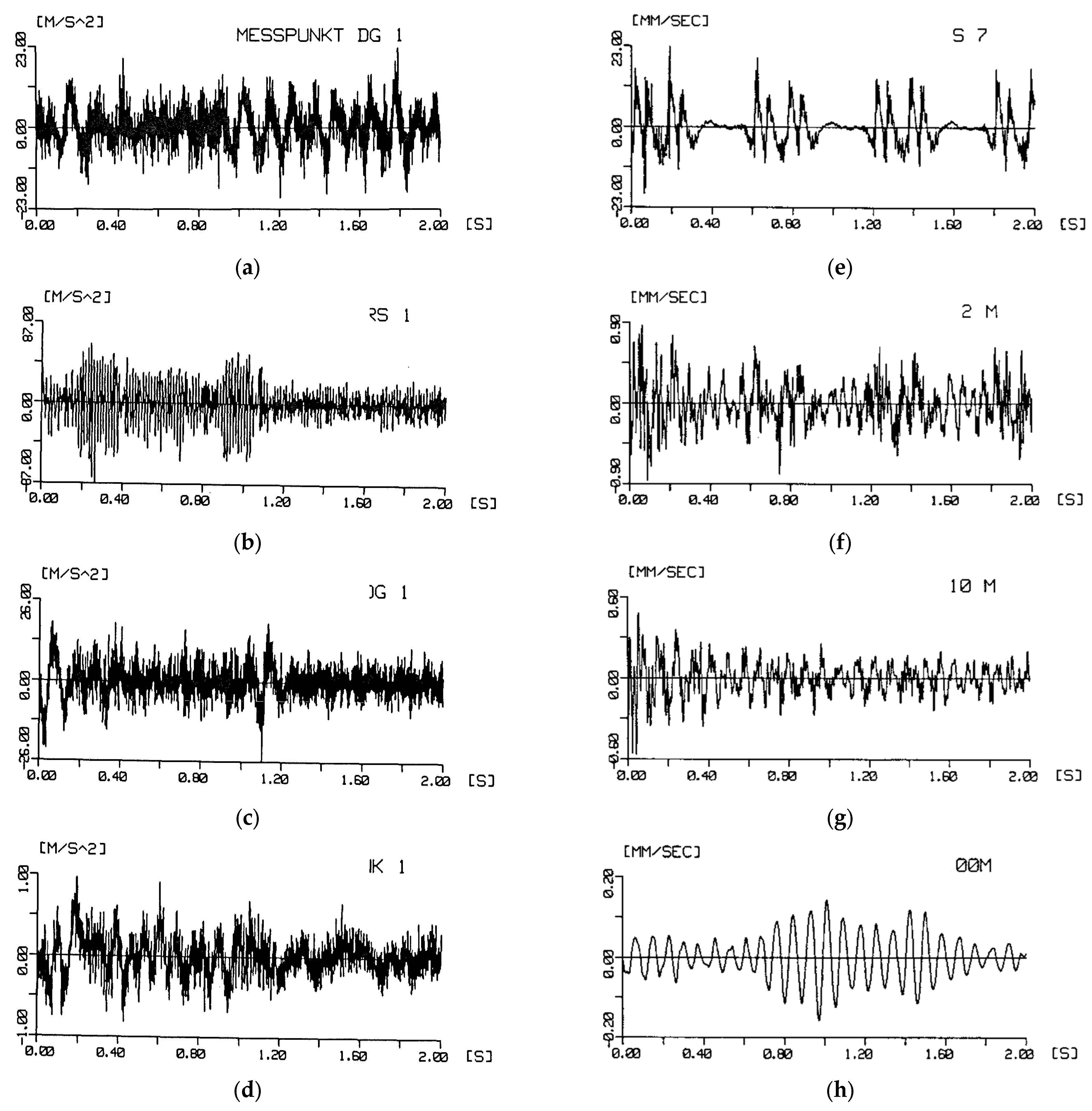
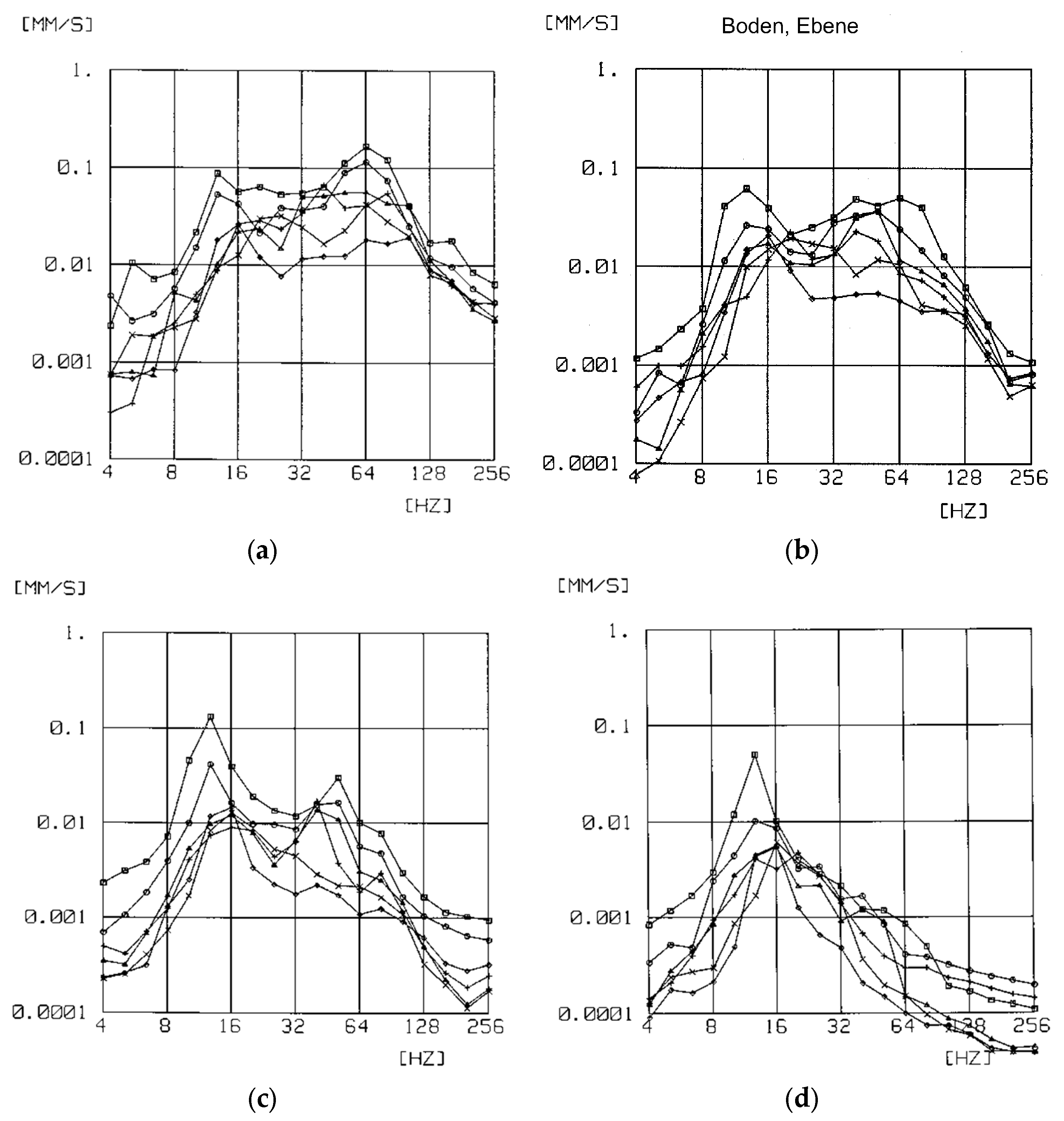
3. One-Third Octave Band Spectra of the Vehicle, Track, Bridge and Soil Vibrations and the Interpretation of Different Frequency Bands

The vibrations of the different systems (vehicle, track, bridge, soil) and the different measurement points are presented as one-third octave band spectra for the different train speeds. At first, the accelerations of the wheelset are analysed in Figure 6. The wheelset spectra at the tunnel track (Figure 6a) start with amplitudes below 1 m/s² at low frequencies, followed by a strong increase and a strong maximum at 63 Hz, and at high frequencies, the accelerations decrease strongly. This is the strongest frequency-dependent behaviour for all the track types. The maximum on the bridge and the surface line (Figure 6c) is not so sharp and a wider high-amplitude range between 63 and 100 Hz is observed. The maximum is due to the vehicle–track resonance where the wheelset is vibrating on the compliant track. The measured track compliances in Appendix A show the different behaviour of the tunnel track with soft rail pads which has little damping and yields the highest resonance amplitudes. The surface track has its high damping from the radiation damping of the soil. Additional relative maxima can be found at the speed-dependent sleeper-passing frequency at 30, 40, 50, 60 and 80 Hz (Figure 6b). The bridge track has the highest amplitude level at high frequencies. The low-frequency wheelset accelerations clearly increase with the train speed, whereas the differences are smaller at high frequencies.

The wheelset accelerations give some information about the excitation of ground vibrations. If the acceleration spectra are divided by the squared circular frequency ω², displacement spectra are obtained which are identical to the irregularity spectra up to the vehicle–track resonance. Around the vehicle–track resonance, the displacements over-estimate the irregularities. On the other hand, the forces that are acting on the track can be estimated by multiplying the accelerations by the wheelset mass (approximately 1500 kg). This is a good estimation above 10 Hz (above the car-body and bogie resonances) and below 100 Hz (where a flexible behaviour of the wheelset is possible). Whereas the forces are nearly constant, the irregularities strongly decrease with frequency (increasing with wavelength). The irregularities stem from track alignment errors at low and mid frequencies, from wheel out-of-roundness at mid and high frequencies and from long wavelength rail roughness at high frequencies, see [34].

The track vibrations are presented as one-third octave band spectra of the velocities of the rail measurement points in Figure 7. The velocity spectra are almost constant with frequency and generally increasing with the train speed. The amplitudes are between 0.3 mm/s for 63 km/h and 3 mm/s for 160 km/h. A characteristic speed-dependent maximum for three one-third octaves can be found, which is from 12 to 20 Hz for 160 km/h. This maximum is due to the impulse from the passage of the static train loads. The related minima (for example at 10 and 25 Hz for 160 km/h) are an effect of the axle sequence in a bogie [3]. Whereas the low frequencies stem from the passage of the static axle loads, the high frequencies are generated by the dynamic axle loads. The tunnel line shows specific amplitudes and dynamic loads around the vehicle–track resonance at 63 Hz. The bridge track has the highest and nearly constant amplitudes at high frequencies whereas the ballast track on the soil surface has the lowest high-frequency level. The sleeper vibrations on the tunnel line (Figure 7b) are only one tenth of the rail amplitudes (Figure 7a). On the bridge and especially on the surface line, the difference between the rail and sleeper amplitudes is smaller due to the stiffer rail pads used for the ballast track. The track slab in the tunnel (Figure 7c) shows similar spectra as the sleepers. All track measurement points in the tunnel have a clear reduction in the frequency range between the speed-dependent axle impulse maximum at 6 to 16 Hz and the vehicle–track resonance at 63 Hz. The vibration amplitudes of the bridge (Figure 7f) are clearly smaller than the rail and the sleeper amplitudes. Peaks at the 6 and 10 Hz one-third octave indicate bridge resonances which are prominent for the 100 km/h and, especially, 160 km/h train speeds, where the amplitudes of 2 mm/s are even higher than the sleeper amplitudes. It is expected that the bridge resonances could also be seen in the ground vibration as has been calculated in [1].

The ground vibrations measured above the tunnel line are presented as one-third octave spectra in Figure 8. As with the amplitudes in Figure 5b, the frequency characteristics of the different measurement points are very similar, and the spectra are only somewhat smaller for the farthest distances. The mid-frequency maxima can be found for 125 and 160 km/h whereas the more dominant high-frequency maximum around 63 Hz is present for all train speeds. The frequency range of this maximum is wider than for the vehicle and the track and includes frequencies from 32 to 80 Hz. The ground-vibration spectra at the surface line vary strongly with the distance from the track. The spectra close to the track (Figure 7i) are almost constant and include the quasi-static component below 8 Hz, at least for the highest train speeds. At 5 m distance (Figure 9a) the quasi-static component has already disappeared and the high-frequency part of the spectrum is dominant. This changes with increasing distance. The high-frequency part from 40 to 80 Hz and the mid-frequency part around 12 Hz are equally important at 17.5 m (Figure 9b) whereas the latter is already dominant at 30 m (Figure 9c). Finally at 100 m, only the peak at 12 Hz is left over (Figure 9d). These characteristics are due to the wave transfer properties of the soil where the material damping reduces the high-frequency content considerably.

4. Detailed Analysis of Tunnel and Bridge Characteristics

The characteristics of the vibrations on the tunnel and bridge lines are analysed by the time histories and the narrow-band spectra in this section, and the consequences will be discussed in Section 6.

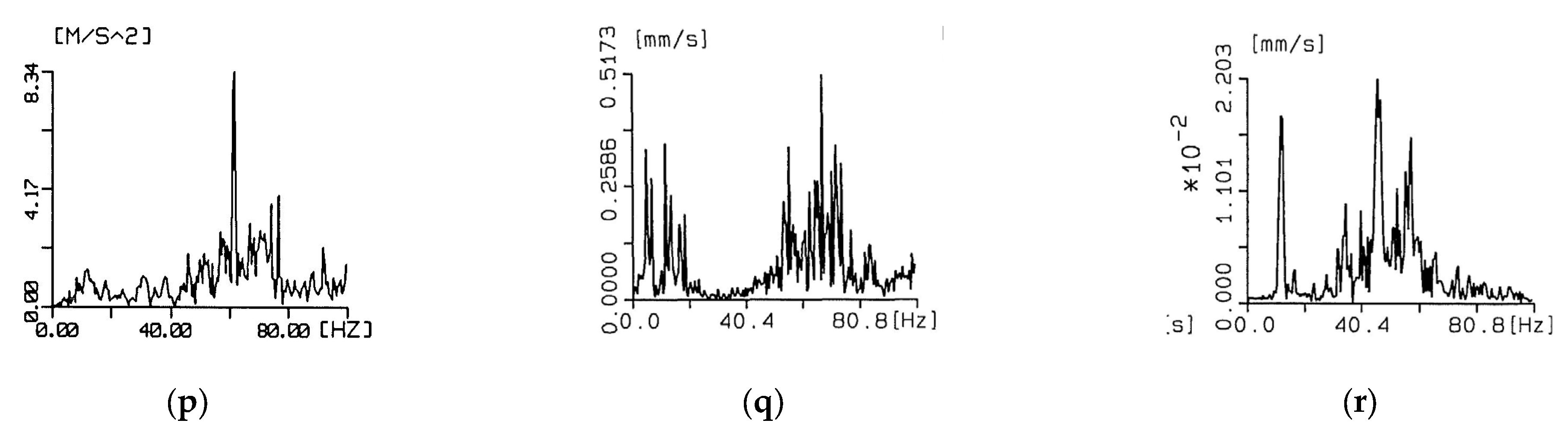
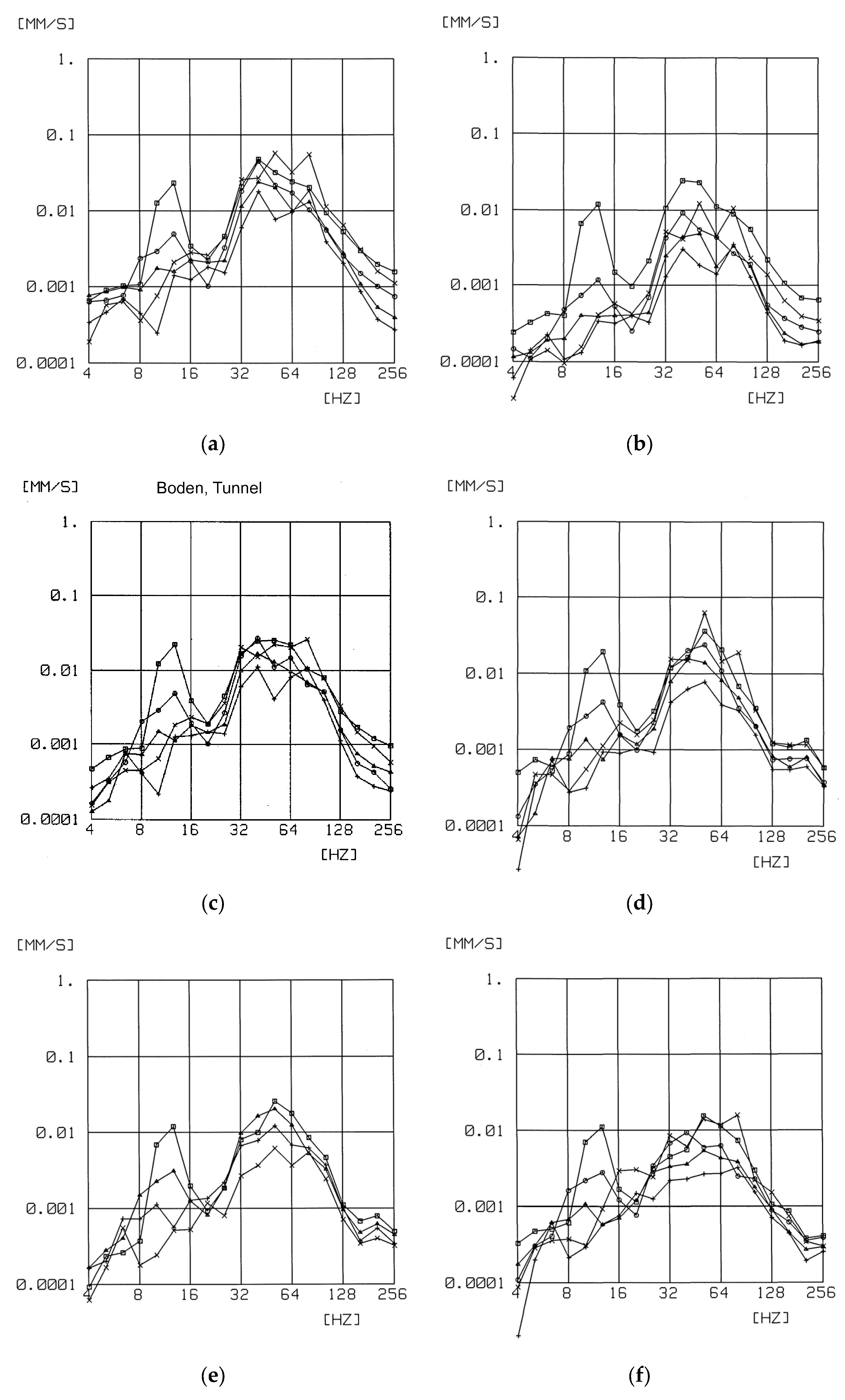
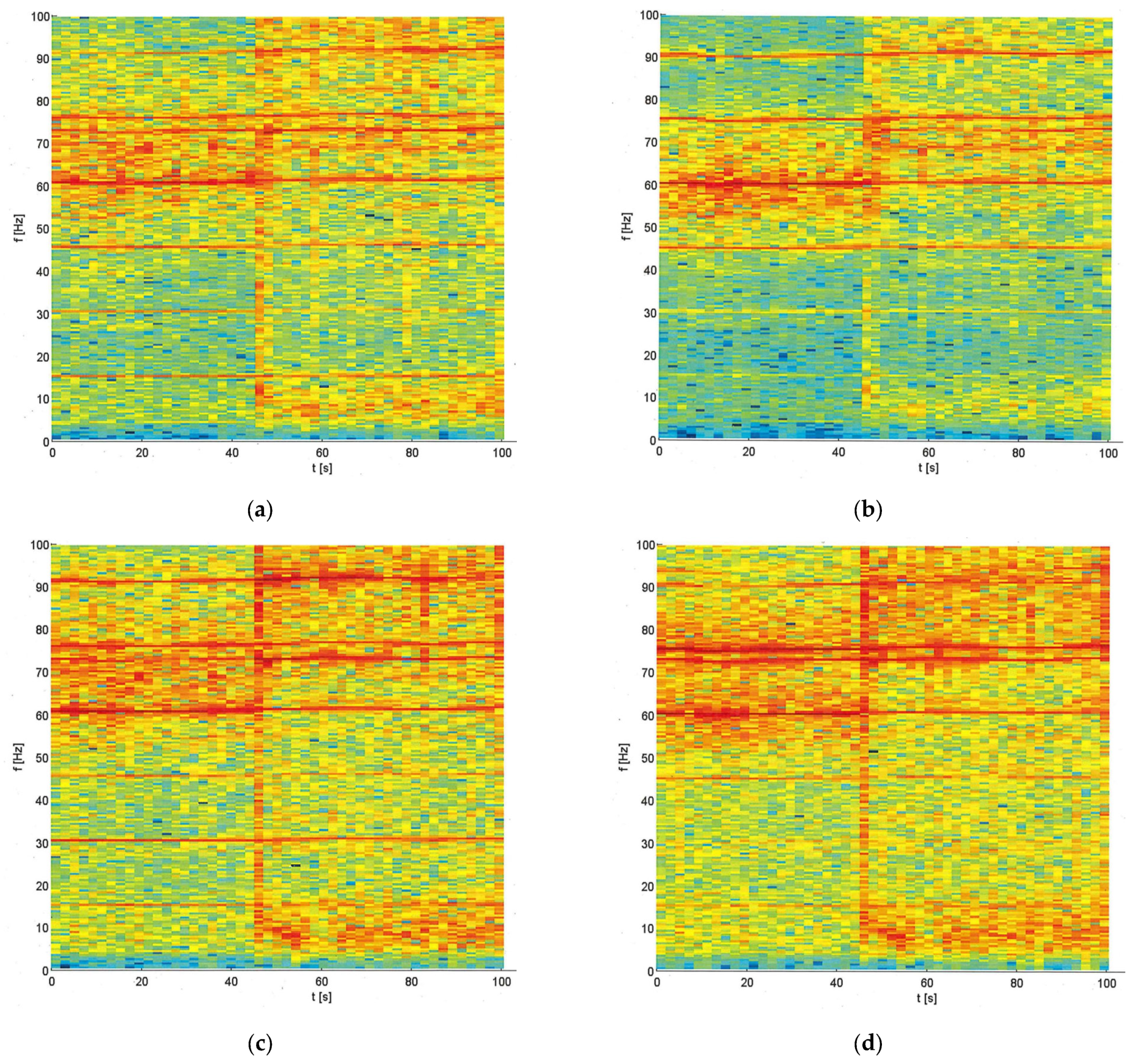
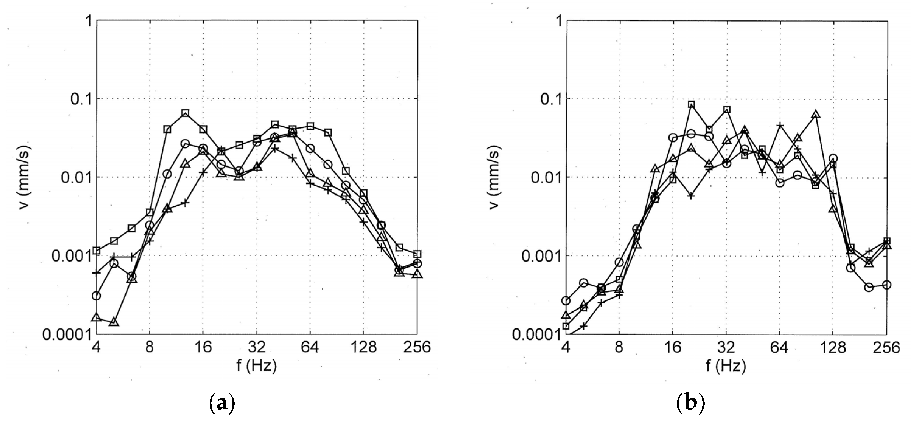
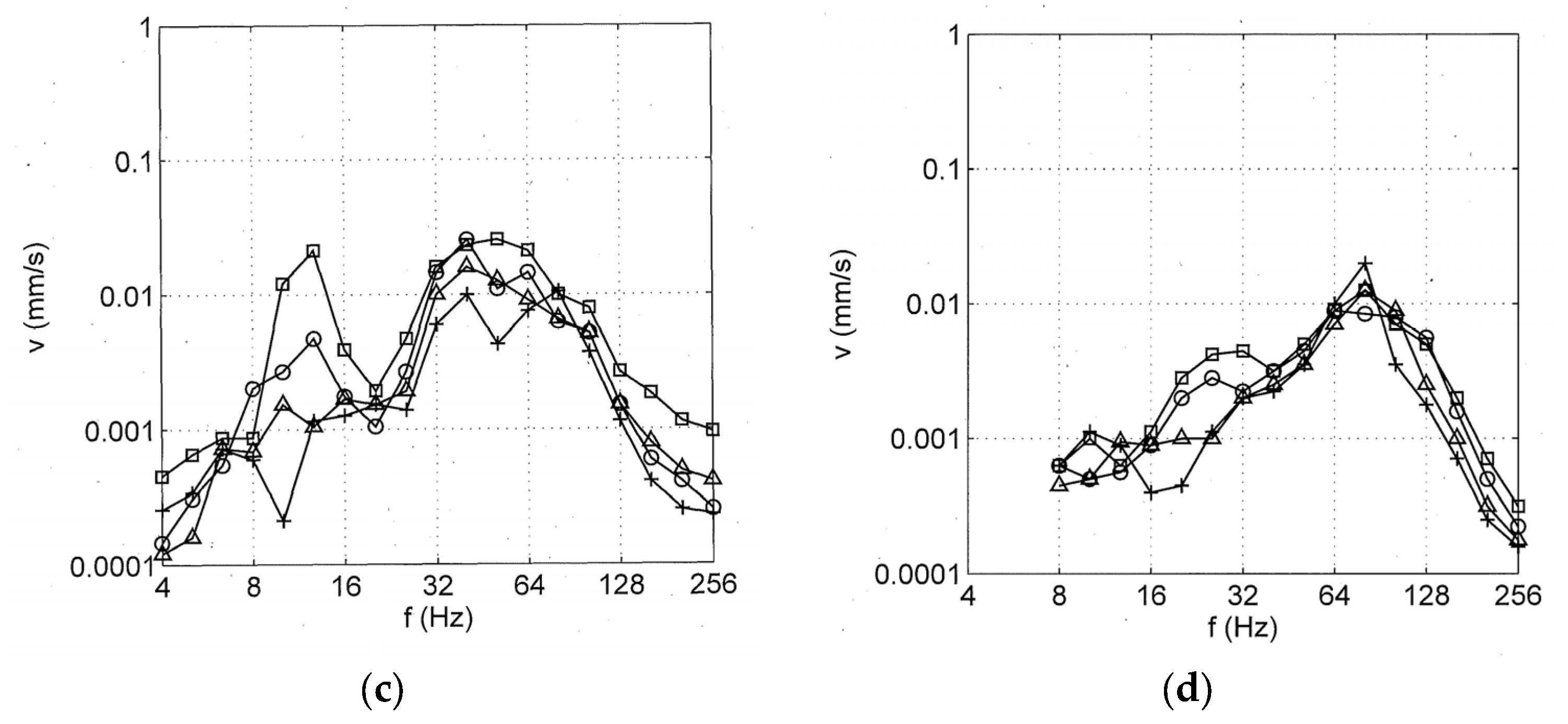
4.1. Narrow-Band Spectra of the Tunnel Vibrations

Firstly, the axle-box accelerations are analysed in a spectrogram plot in Figure 10. The time-dependent Fourier spectra are shown for the slab track in the tunnel up to t = 45 s and for the ballast track at the surface track for t > 45 s. The Fourier spectra of all four wheels of a bogie show regular maxima at about 15, 30, 45, 60, 75 and 90 Hz which are due to the wheel out-of-roundness. The additional maximum at f_S = 72 Hz close to the fifth out-of-roundness frequency is due to the sleeper distance and the train speed of 160 km/h. Besides these common characteristics, clear differences between the tunnel and the surface line can be observed. On the slab track in the tunnel, the frequencies between 60 and 75 Hz are amplified whereas higher frequencies between 75 and 90 Hz are dominant on the surface line, which indicates the higher vehicle–track resonance for the ballasted track. The increased amplitudes below 10 Hz are generated by the higher irregularities of the ballast track. The four different wheels have different out-of-roundness components. In Figure 10a the first order out-of-roundness is stronger, in Figure 10c the second and in Figure 10b the third and the sixth component. The out-of-roundness in the frequency range between 60 and 80 Hz are usually increased by the vehicle–track interaction of the slab track in the tunnel. The axle-box accelerations of different train speeds are presented in Figure 11 as Fourier spectra. The discrete peaks from the out-of-roundness of the wheel are clearest for the low train speeds of 63 and 80 km/h (Figure 11a,d). For higher train speeds, only a few out-of-roundness peaks dominate. For 125 km/h, the sleeper passage is most clearly visible at 60 Hz where it is amplified by the wheelset–track resonance. The wheelset–track resonance can also be found for 160 km/h in Figure 11p.

The Fourier spectra of the slab track and the soil above the tunnel are analysed for the different train speeds on the mid and right-hand side of Figure 11. The characteristic high-frequency range can be clearly found for these measurement points, but they are modified by the different transfer functions of the track and the soil. The sleeper point shows generally a wider frequency band from 50 to 80 Hz, and, for the soil point, the band has lower frequencies between 30 and 60 Hz. The high frequencies above 60 Hz are probably reduced because of the stronger damping effect of the soil. In the amplified frequency range between 30 and 40 Hz, no peak or maximum, which is unique for all train speeds and which would indicate a resonance of the soil, could be found. The smooth maximum of the transfer function of the soil seems to be the reason for the raised amplitudes at this frequency range. In the soil, the peaks from the wheel irregularities can be found at speed-dependent out-of-roundness frequencies, for example at 40, 50 and 60 Hz for the 100 km/h train speed (Figure 11i) or at 32, 40, 48 and 56 Hz for 80 km/h (Figure 11f). On the track, the out-of-roundness components are not sharp peaks but wider frequency bands due to the Doppler effect for moving loads. A characteristic low- to mid-frequency band occurs which is shifted with increasing train speed and which is due to the passage of the static axle loads. Six peaks are visible for the higher speeds which are related to the specific axle sequence of the test train. A similar component is also present at the soil surface mainly for the highest train speed. This similarity of the track and the soil spectra is even stronger for the surface line and it has been analysed for high-speed measurements in [3].

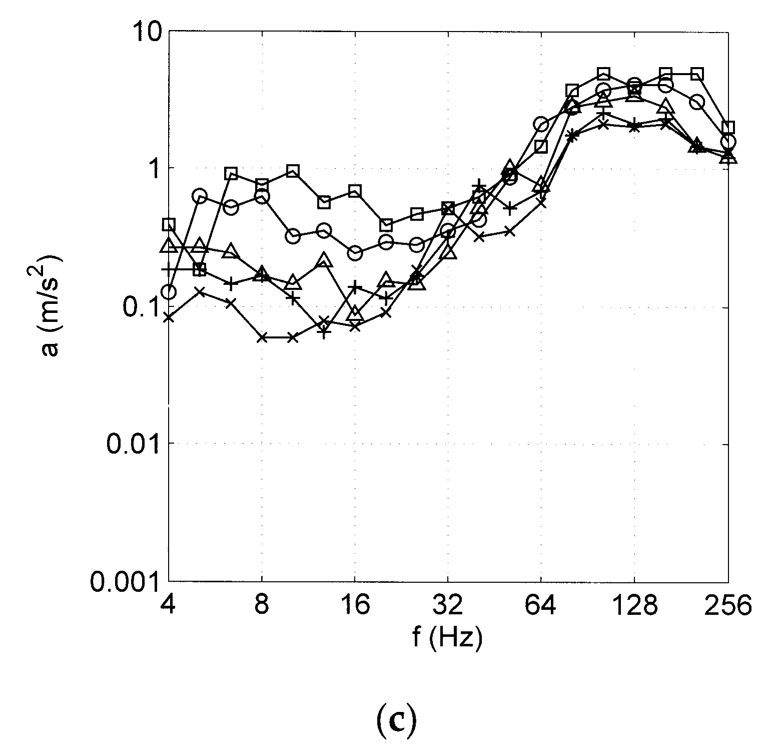
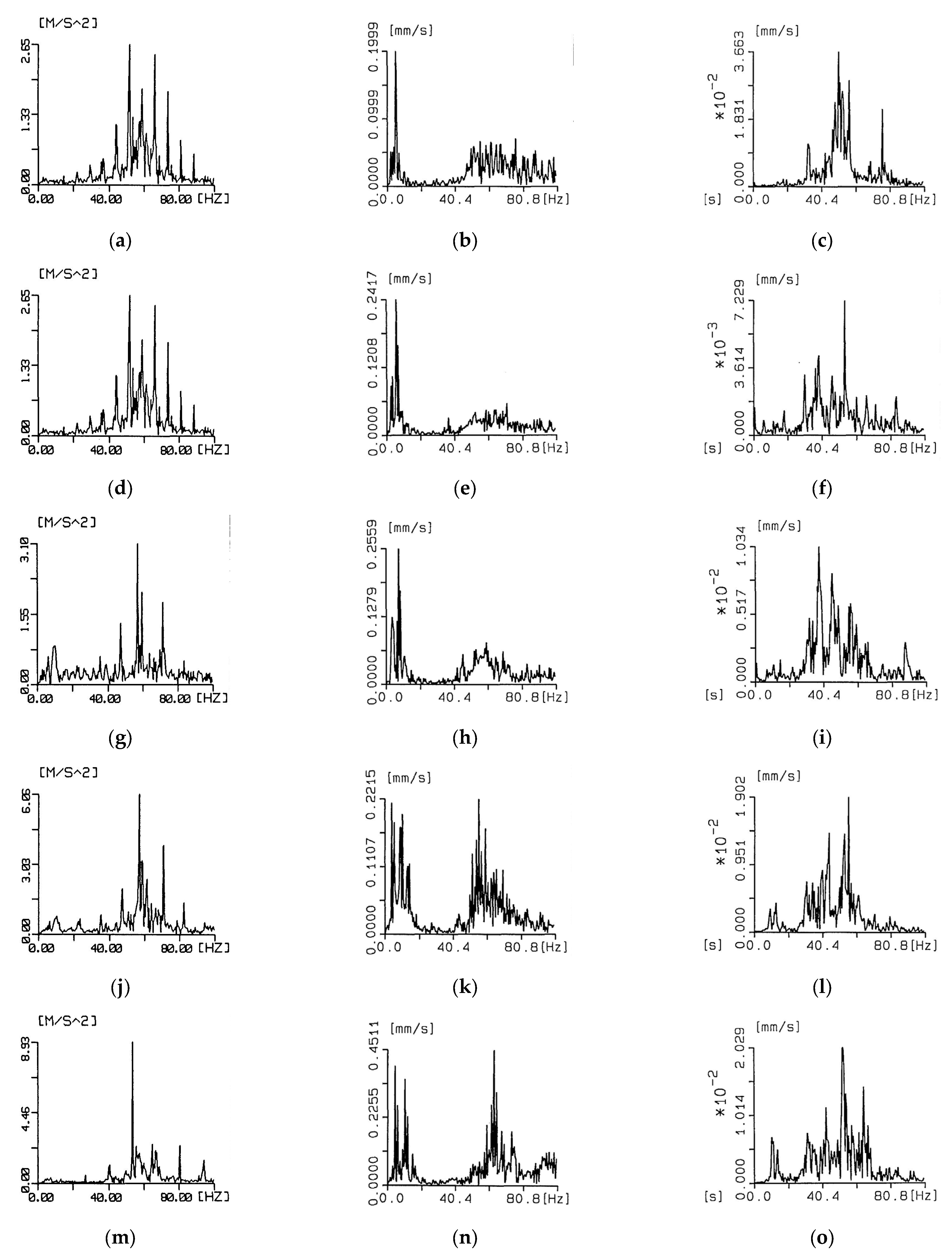
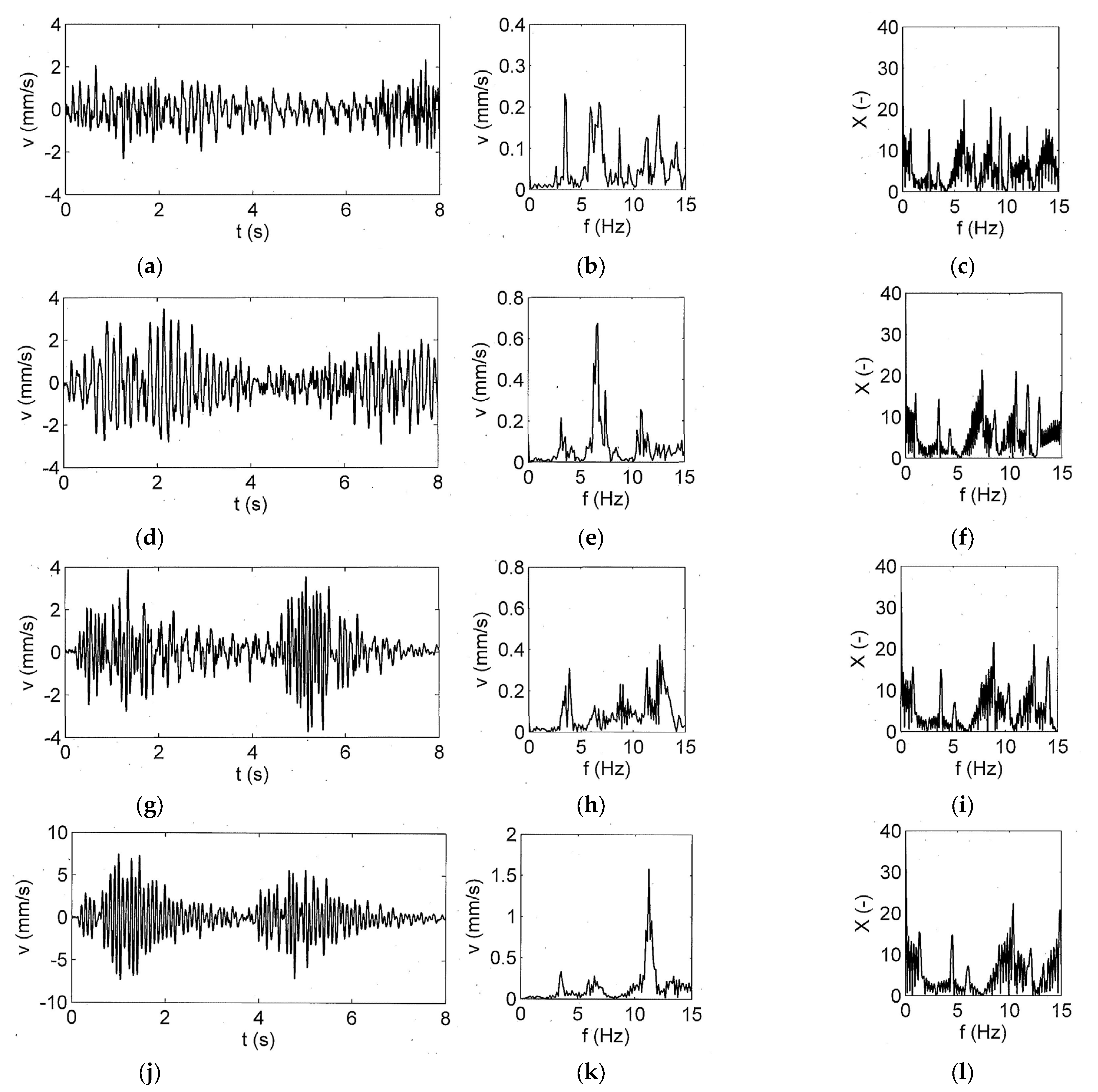
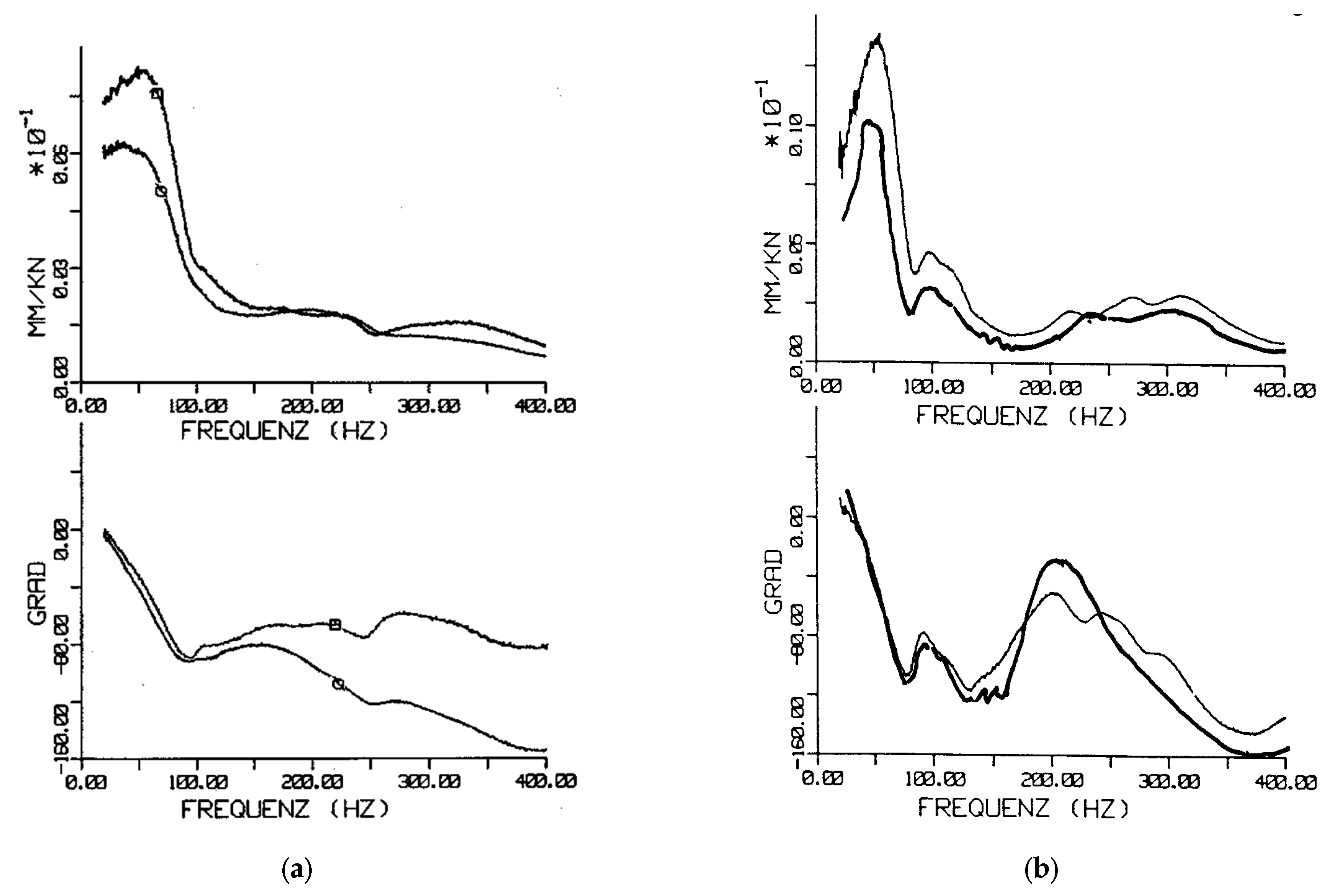
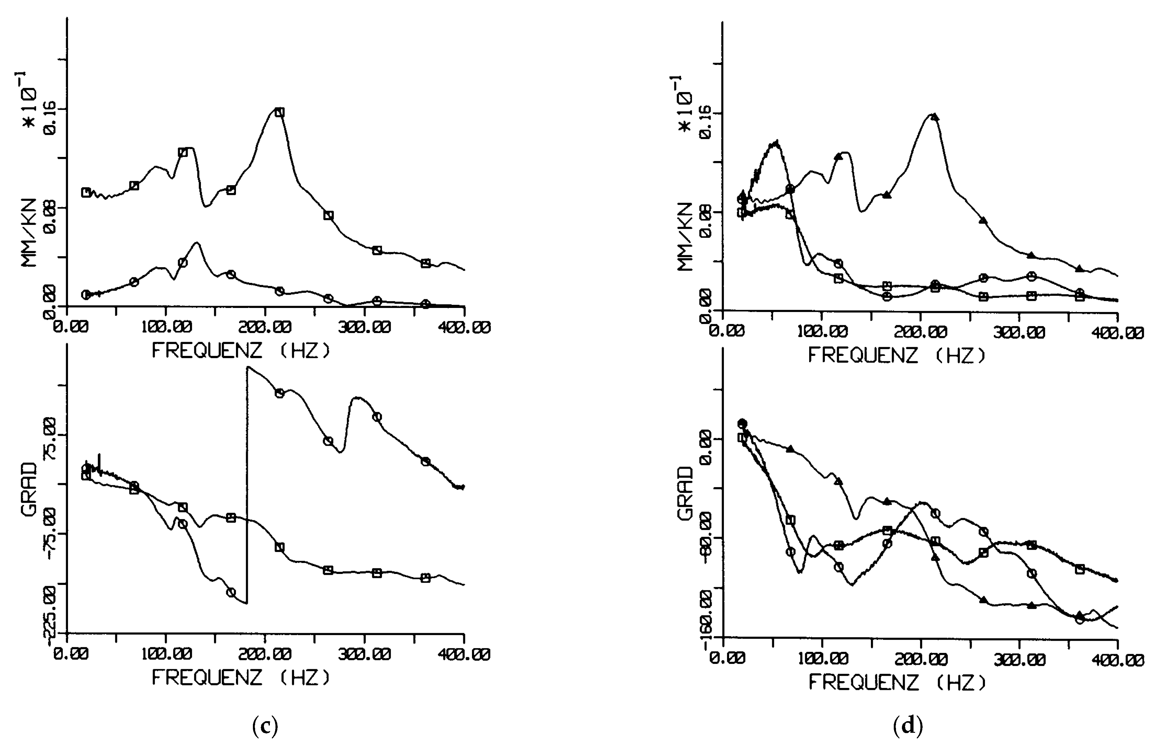
4.2. Time Histories and Narrow-Band Spectra of The Bridge Vibrations

Figure 12 compiles the detailed results for the bridge for five train speeds, the time histories in the left column (Figure 12a,d,g,j,m), the corresponding Fourier spectra in the second column (Figure 12b,e,h,k,n) and the axle sequence spectra in the third column (Figure 12c,f,i,l,o). The axle sequence of the seven-unit test train is calculated according to the formula:

$$X(\omega )=\left|\sum _{k=1}^n{A}_k \exp (-i\omega T_k)\right|$$

where A_k is a non-dimensional load factor (A_k = 1 for the passenger cars and A_k = 2 for the locomotives) and T_k = x_k/v_T is the delay time of the k-th axle at position x_k along the train. The lowest pair of peak frequencies can be found for all train speeds, for example at 5 and 6 Hz for 160 km/h (Figure 12n). The highest pair of peak frequencies are clearly visible for example at 13 and 14 Hz for 125 km/h (Figure 12h). The bridge response is strongly influenced by this axle sequence and by the different natural frequencies which are at 3.5 Hz (first bending mode), 7 Hz (first torsional mode), 11 Hz (second bending mode) and 13.5 Hz (second torsional mode), see [2]. The spectrum of the bridge response v_j(ω) for mode j can be represented as a product of three spectra:

$$v_j(\omega )=F_S{W}_j(\omega )H_j(\omega )X(\omega )$$

where X(ω) is the axle sequence spectrum of the train, which is independent of the specific bridge, and H_j(ω) is the bridge transfer function and W_j(ω) is the modal force spectrum, which are independent of the specific train, and F_S = 100 kN. If the resonance frequency ω_j in H_j(ω) meets the maximum (minimum) region of the axle sequence spectrum X(ω), the corresponding resonance v_j(ω_j) is amplified (reduced). The first torsional mode at 7 Hz is clearly raised for the train speed of 100 km/h (Figure 12d) whereas the second bending mode at 11 Hz is dominant for 140 km/h (Figure 12j). At the same train speeds, the other bridge modes are cancelled as they lie in a minimum region of the axle sequence spectrum. As a result, the time histories on the left look almost mono-frequent with 7 Hz for 100 km/h and with 11 Hz for 140 km/h. For the other train speeds, two modes are excited at the same time, but not so strongly: the first and second mode for 80 km/h, the first and fourth mode for 125 km/h and the third and fourth mode for 160 km/h. As indicated in [1], the bridge resonances are also present and probably dominant in the ground vibration.

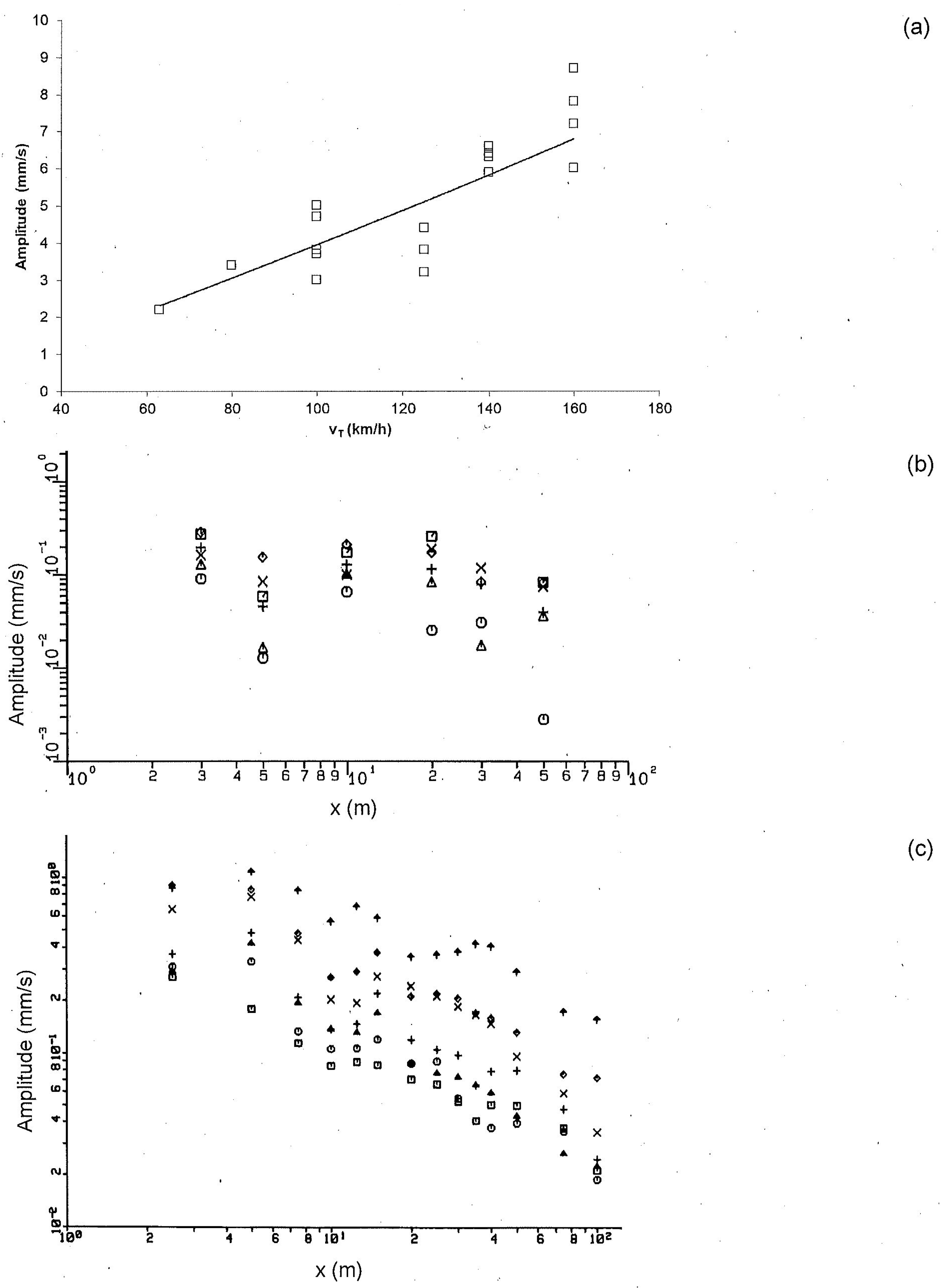
5. The Amplitudes and The Amplitude Ratio of The Ground Vibrations from the Tunnel and the Surface Line for Normal and High Train Speeds

In this section, the amplitudes of the tunnel and the surface line are compared directly where the amplitudes for all train speeds are shown in Figure 13a,b for the tunnel line and in Figure 13c,d for the surface line. In addition to the passages of the normal passenger train with low speeds (Figure 13a,c), the high-speed passages of the Intercity Experimental at the same sites are presented in Figure 13b,d. For all four measurement series, two main frequency ranges can be observed. A high-frequency range from 30 to 80 Hz (Figure 13a,c) or 64 to 128 Hz (Figure 13b,d) includes the sleeper-passage component and the vehicle–track resonance which is dominant for the tunnel measurements. A mid-frequency component is strongest for the high-speed train on the surface line which ranges from 20 to 32 Hz, 16 to 25 Hz, 12 to 20 Hz and 10 to 16 Hz depending on the train speed (Figure 13d). This mid-frequency component can also be found for the passenger train with 125 and 160 km/h in Figure 13a,b. It is clearly reduced for the high-speed train in the tunnel (Figure 13c). From these ground vibration measurements, the frequency-dependent surface-to-tunnel reduction v_T/v_S has been evaluated in Figure 14 where the velocity amplitudes v_T near the tunnel are divided by the velocity amplitudes v_S near the surface line. The low-and high-frequency tunnel-to-surface ratios come close to one. A significant reduction was found in the mid-frequency range between 10 and 25 Hz for the low speeds (Figure 14a) and between 12 and 50 Hz for the high speeds (Figure 14b). The reduction goes down to v_T/v_S = 0.1 or even 0.03 for certain high-speed frequencies.

The surface-to-tunnel amplitude ratios of other institutes are collected in Figure 14c. The Highspeed2 prediction [35] uses a similar strong surface-to-tunnel reduction between 16 and 32 Hz for high-speed traffic in deep bored tunnels (square markers). Measurements of the Karlsruhe Institute of Technology [29] at a near-surface tunnel showed a reduction down to 0.1 between 12 and 32 Hz (triangle markers). The most complete measurements were performed by the Austrian Institute of Technology [31] where shaker excitation was used to measure the transfer function from the surface or (deep) tunnel track to the measurement points at the surface. From the measured ground vibrations from train passages and the transfer functions of the soil, forces have been back calculated and a comparison has been established based on these forces. The soil on the surface line has higher transfer values between 16 and 32 Hz so that the originally lower tunnel–surface ratios have been corrected to higher values of v_T/v_S = 0.3 (circle markers). All three high-speed measurements (Figure 14c) and the measurements of BAM (Figure 14a,b) agree well in the reduction of the mid-frequency component. Moreover, all measurements show a higher high-frequency tunnel-to-surface ratio. The high-frequency ratios are around the value one, somewhat lower for the German measurements and somewhat higher for the Austrian measurements. This high-frequency range starts between 32 and 50 Hz, and it is based on significantly high amplitudes on the tunnel and surface lines.

6. Discussion of The Bridge and Tunnel Characteristics

The specific behaviours of the tunnel and bridge tracks from the measurements can be combined with the theoretical results in [1]. It has been shown that the bridge resonances would also be dominant in the ground vibration, see also [13]. Special bridge resonances were found in the time histories and narrow-band spectra in Section 4.2, which are strongly influenced by the speed-dependent axle sequence spectra of the train. The first torsional resonance at 7 Hz and the second bending resonance at 11 Hz have been amplified by the frequency range related to the axle distance in a bogie. The first bending mode of this 45 m long bridge is at 3.5 Hz whereas the standard viaduct bridges in China and Taiwan with a shorter span length of 32 m and 30 m, respectively, have their first bending eigenfrequency at about 5 Hz according to [14,16]. In [16,21], measured and calculated ground vibrations are shown for 100 and 200 m distance which have their dominant frequencies below 10 Hz and show some resonance effects for train speeds between 220 and 300 km/h. For lower train speeds of 120 to 200 km/h, a maximum at 16 Hz has been found in [19] which dominates the ground vibrations and is probably due to the second bending resonance of the standard Chinese viaduct. Bridge resonances and their effects on the ground vibrations have also been found for freight trains [20] and for local trains [21].

The bridge response has often been measured for long high-speed trains and the regular car-length frequencies dominate the Fourier spectra of the bridge and ground vibrations. Whereas in [21], the first to third car-length frequency is dominant in the far field velocities, the near field accelerations in [17] showed dominant peaks at the 7th, 9th–11th and 13th car-length frequency. These high-speed measurements confirm the strong effect of the axle sequence spectrum on the bridge response which has been stated for the present measurements of normal train speeds. The short continuous viaduct bridges in Japan have higher bridge resonance frequencies so that only the axle sequence peaks can be found in the low-frequency range [18].

For the tunnel line, the theoretical results in [1] show a reduction effect at high frequencies due to the excitation at depth and the wider load distribution across the tunnel invert. Therefore, the strong high-frequency amplitudes in the measurements can only be explained by a stronger excitation. The detailed analysis in Section 4.1 and in Appendix A show no special eigenmodes of the track slab in this frequency range, but the impact response shows a reduced radiation damping of the slab track with soft rail pads (Figure 15c) so that the combined wheelset–track resonance and the sleeper-passage component are stronger on the tunnel line.

A reduction effect of the tunnel line at mid frequencies has been clearly measured by BAM and other institutes. This cannot be explained by the theoretical reduction in [1] which starts at higher frequencies. A smaller excitation due to smaller irregularities of the slab track would be a possible explanation, but this holds for the whole low-frequency range and not only for the specific mid-frequency range which has been observed in all measurements. The soil at the tunnel depth could be stiffer than at the surface and result in smaller amplitudes, but it is not probable that this holds for all measurements that have been reported here. Moreover, the strong mid-frequency ground vibration component on the surface line cannot be found in the axle-box accelerations in Figure 10, so there are no dynamic loads which could excite this component. It must be concluded that the mid-frequency ground vibration is excited by the static loads. The moving static loads yield axle impulses on the track which would superpose to the quasi-static response of the near-field soil with very low frequencies (Figure 7f). In the far field, some scattered parts of the axle impulses can be left over due to irregularities of the ballast and the soil [34]. These scattered axle impulses constitute the mid-frequency ground vibration component for the surface line. On the tunnel line, the axle loads are distributed wider along the track so that the axle impulses are longer and have a reduced high-frequency content. This missing high-frequency content would clearly explain the mid-frequency surface-to-tunnel reduction of the measurements. There is no special reduction effect of the tunnel, but an additional special ground vibration component must be considered for the surface line.

7. Conclusions

A unique measurement campaign has been performed on tunnel, bridge and surface lines. The vibrations of the vehicle, track, bridge and the ground have been analysed dependent on train speeds between 60 and 160 km/h. The specific results are the amplification and reduction of the bridge resonances which have been related to the maxima and minima amplitude regions of the speed-dependent axle sequence spectrum of the test train which has not been used in bridge analysis so far. With this, it could be explained why the first torsional mode at 7 Hz is dominant for a train speed of 100 km/h, and the second bending mode at 11 Hz is dominant for 140 km/h whereas the other modes are cancelled in both cases. The bridge resonances are expected to be also dominant in the ground vibration around the bridge. For the tunnel line, the simultaneously measured vehicle, track and ground vibrations all show a strong high-frequency range between 30 and 80 Hz which has been explained by the dominant speed-dependent sleeper-passage component and the weakly damped vehicle–track resonance at about 60 Hz. The low- and mid-frequency amplitudes are considerably smaller above the tunnel line compared to the surface line. This frequency range can clearly be found for the track measurement points, where the passing static axle loads are the dominant excitation, and at the ground around the surface line. The regular low-frequency quasi-static response occurs in the near field, whereas it disappears in the far field where the scattering of the axle pulses by a randomly varying soil is the reason for the mid-frequencies. The scattered axle impulses are reduced or suppressed by the wider distribution of the load along the tunnel line. Therefore, a strong mid-frequency tunnel-to-surface reduction has been consistently established by the present measurements and the measurements of other institutes. The explanation of the surface-to-tunnel differences is an important novelty of this article.

References

1. Auersch, L. Reduction of train-induced vibrations—Calculations of different railway lines and mitigation measures in the transmission path. Appl. Sci. 2023, 13, 6706. [Google Scholar] [CrossRef]
2. Auersch, L.; Said, S.; Rücker, W. Das Fahrzeug-Fahrweg-Verhalten und die Umgebungserschütterungen bei Eisenbahnen; Research Report 243; BAM: Berlin, Germany, 2001.
3. Auersch, L. The excitation of ground vibration by rail traffic: Theory of vehicle-track-soil interaction and measurements on high-speed lines. J. Sound Vib. 2005, 284, 103–132. [Google Scholar] [CrossRef]
4. Iwnicki, S. Handbook of Railway Vehicle Dynamics; Taylor & Francis: Abingdon, UK, 2006. [Google Scholar]
5. Milne, D.; Le Pen, L.; Watson, G.; Thompson, D.; Powrie, W.; Hayward, M.; Morley, S. Monitoring and repair of isolated trackbed defects on a ballasted railway. Transp. Geotech. 2018, 17, 61–68. [Google Scholar] [CrossRef]
6. Unsiwilai, S.; Wang, L.; Núnez, A.; Li, Z. Multiple-axle box acceleration measurements at railway transition zones. Measurement 2023, 213, 112688. [Google Scholar] [CrossRef]
7. Lourenco, A.; Ferraz, C.; Ribeiro, D.; Mosleh, A.; Montenegro, P.; Vale, C.; Meixedo, A.; Marreiros, G. Adaptive time series representation for out-of-round railway wheels fault diagnosis in wayside monitoring. Eng. Fail. Anal. 2023, 152, 107433. [Google Scholar] [CrossRef]
8. Fryba, L. Vibration of Solids and Structures under Moving Loads; Springer: Berlin/Heidelberg, Germany, 1973. [Google Scholar]
9. Savin, E. Dynamics of Railway Bridges under Moving Loads. PhD Thesis, Ecole Centrale de Paris, Gif-sur-Yvette, France, 1994. [Google Scholar]
10. Yang, Y.; Yau, J.; Hsu, J. Vibration of simple beams due to trains moving at high speeds. Eng. Struct. 1997, 19, 936–944. [Google Scholar] [CrossRef]
11. Yang, Y.; Lin, C.; Yau, J.; Chang, D. Mechanism of resonance and cancellation for train-induced vibrations on bridges with elastic bearings. J. Sound Vib. 2004, 269, 345–360. [Google Scholar] [CrossRef]
12. Museros, P.; Moliner, E.; Martinez-Rodrigo, M. Free vibrations of simply supported beam bridges under moving load: Maximum resonance, cancellation and resonant vertical acceleration. J. Sound Vib. 2013, 332, 326–345. [Google Scholar] [CrossRef]
13. Wu, Y.; Yang, Y. A semi-analytical approach for analyzing ground vibrations caused by trains moving over elevated bridges. Soil Dyn. Earthq. Eng. 2004, 24, 949–962. [Google Scholar] [CrossRef]
14. Xia, H.; Zhang, N.; Guo, W. Analysis of resonance mechanism and conditions of train-bridge system. J. Sound Vib. 2006, 297, 810–822. [Google Scholar] [CrossRef]
15. Galvín, P.; Romero, A.; Moliner, E.; De Roeck, G.; Martinez-Rodrigo, M. On the dynamic characterisation of railway bridges through experimental testing. Eng. Struct. 2020, 226, 111261. [Google Scholar] [CrossRef]
16. Ju, S.; Lin, H. Experimentally investigating finite element accuracy for ground vibrations induced by high-speed trains. Eng. Struct. 2008, 30, 733–746. [Google Scholar] [CrossRef]
17. Xing, M.; Wang, P.; Zhao, C.; Wu, X.; Kang, X. Ground-borne vibration generated by high-speed train viaduct systems in soft-upper/hard-lower rock strata. J. Cent. South Univ. 2021, 28, 2140–2157. [Google Scholar] [CrossRef]
18. Takemiya, H.; Bian, X. Shinkansen high-speed train induced ground vibrations in view of viaduct–ground interaction. Soil Dyn. Earthq. Eng. 2007, 27, 506–520. [Google Scholar] [CrossRef]
19. Liu, Q.; Zhang, X.; Zhang, Z.; Li, X. In-situ measurement of ground vibration induced by inter-city express train. Appl. Mech. Mater. 2012, 204–208, 502–507. [Google Scholar] [CrossRef]
20. Hu, J.; Luo, Y.; Xu, J. Experimental and numerical analysis and prediction of ground vibrations due to heavy haul railway viaduct. Math. Probl. Eng. 2019, 2019, 2751815. [Google Scholar] [CrossRef]
21. Ju, S.; Lin, H.; Huang, J. Dominant frequencies of train induced vibrations. J. Sound Vib. 2009, 319, 247–259. [Google Scholar] [CrossRef]
22. Duval, G. Cartographie des Champs Vibratoires à la Surface des Sols en Milieu Urbain: Application Ferroviaire et Chantiers. Ph.D. Thesis, Université de Lyon, Lyon, France, 2022. [Google Scholar]
23. Chatterjee, P.; Degrande, G.; Jacobs, S.; Charlier, J.; Bouvet, P.; Brassenx, D. Experimental results of free field and structural vibrations due to underground railway traffic. In Proceedings of the 10th International Congress on Sound and Vibration (ICSV28), Stockholm, Sweden, 7–10 July 2003; pp. 1–8. [Google Scholar]
24. Degrande, G.; Schevenels, M.; Chatterjee, P.; Van de Velde, W.; Hölscher, P.; Hopman, V.; Wang, A.; Dadka, N. Vibrations due to a test train at variable speed in a deep bored tunnel embedded in London clay. J. Sound Vib. 2006, 293, 626–644. [Google Scholar] [CrossRef]
25. Gupta, S.; Lombaert, G.; Degrande, G. Experimental validation of a numerical model for subway induced vibrations. J. Sound Vib. 2009, 321, 786–812. [Google Scholar] [CrossRef]
26. Jin, Q.; Thompson, D.; Lurcock, D.; Toward, M.; Ntotsios, E. A 2.5D finite element and boundary element model for the ground vibration from trains in tunnels and validation using measurement data. J. Sound Vib. 2018, 422, 373–389. [Google Scholar] [CrossRef]
27. Xing, M.; Zhao, C.; Wang, P.; Lu, J.; Yi, Q. A numerical investigation of ground vibration induced by typical rail corrugation of underground subway. Shock. Vib. 2019, 2019, 8406813. [Google Scholar]
28. Heckl, M.; Hauck, G.; Wettschureck, R. Structure-borne sound and vibration from rail traffic. J. Sound Vib. 1996, 193, 175–184. [Google Scholar] [CrossRef]
29. Kurze, U.; Wettschureck, R. Erschütterungen in der Umgebung von flach liegenden Eisenbahntunneln im Vergleich mit freien Strecken. Acustica 1985, 58, 170–176. [Google Scholar]
30. Jurdic, V.; Bewes, O.; Greer, R. Developing prediction model for ground-borne noise and vibration from high speed trains running at speeds in excess of 300 km/h. In Proceedings of the 21st International Congress on Sound and Vibration (ICSV21), Beijing, China, 13–17 July 2014; pp. 1–9. [Google Scholar]
31. Tappauf, B.; Alten, K. Erschütterungsprognose an der Bahn—Aktuelle Methoden. In VDI Bericht “Baudynamik 2022”; VDI-Verlag: Düsseldorf, Germany, 2022; pp. 177–194. [Google Scholar]
32. Said, S.; Auersch, L.; Rücker, W. Messungen der Fahrwegschwingungen und der Erschütterungen bei Versuchsfahrten des Intercity-Experimental; Technical Report TV 8214: Rückwirkung und Erschütterungsausbreitung; BAM: Berlin, Germany, 1988.
33. Willenbrink, L. Körperschallmessungen über dem Mühlbergtunnel im Rahmen der ICE-Versuchsfahrten auf der NBS Hannover Würzburg; Report 75676; DB-Versuchsanstalt: Munich, Germany, 1987. [Google Scholar]
34. Auersch, L. Different types of continuous track irregularities as sources of train-induced ground vibration and the importance of the random variation of the track support. Appl. Sci. 2022, 12, 12031463. [Google Scholar] [CrossRef]
35. Hood, R.; Greer, R.; Breslin, M.; Williams, P. The calculation and assessment of ground-borne noise and perceptible vibration from trains in tunnels. J. Sound Vib. 1996, 193, 215–225. [Google Scholar] [CrossRef]
Figure 1. Measurement sections at (a,b) the bridge, (c,d) surface and (e,f) tunnel lines, cross sections (a,c,e) and view from the test train (b,d,f).
Applsci 13 10992 g001aApplsci 13 10992 g001b
Figure 2. Measurement points on the bridge and surface sections.
Applsci 13 10992 g002
Figure 3. Measurement points on the tunnel section.
Applsci 13 10992 g003
Figure 4. Measured accelerations of the vehicle (ad) and velocities of the track and soil (eh); (a) bogie in the tunnel, (b) wheel/axle-box, (c) bogie and (d) car body on the bridge; (e) sleeper and soil at (f) 2.5 m, (g) 10 m and (h) 100 m distance from the surface track.
Applsci 13 10992 g004
Figure 5. Maximum amplitudes (a) of the bridge as a function of the train speeds, (b) above the tunnel as a function of the horizontal distance, as a function of the distance and train speeds: ☐ 63, ○ 80, △ 100, + 125, ✕ 140, ◇ 160 km/h, and (c) on the surface line as a function of the distance and train speeds: ☐ 40, ○ 63, △ 80, + 100, ✕ 125, ◇ 140, ▽ 160 km/h.
Applsci 13 10992 g005
Figure 6. One-third octave band spectra of the axle-box accelerations on the (a) tunnel, (b) bridge and (c) surface lines, for different train speeds ☐ 160, ○ 125, △ 100, + 80, ✕ 63 km/h.
Applsci 13 10992 g006aApplsci 13 10992 g006b
Figure 7. One-third octave band spectra of the rail (a,d,g), the sleeper (b,e,h) and environmental (c,f,i) velocities, (ac) tunnel, (df) bridge and (gi) surface line, track slab (c), one-third point of the bridge deck (f), near field of the surface track (2.5 m), (i), for different train speeds: ☐ 160, ○ 125, △ 100, + 80, ✕ 63 km/h.
Applsci 13 10992 g007
Figure 8. Vibrations of the soil above the tunnel at horizontal distances of (a) 3 m, (b) 5 m, (c) 10 m, (d) 20 m, (e) 30 m and (f) 50 m, one-third octave band spectra for different train speeds: ☐ 160, ○ 125, △ 100, + 80, ✕ 63 km/h.
Applsci 13 10992 g008
Figure 9. Vibrations of the soil at horizontal distances from the surface track (a) 5 m, (b) 17.5 m, (c) 30 m and (d) 100 m, one-third octave band spectra for different train speeds: ☐ 160, ○ 125, △ 100, + 80, ✕ 63 km/h.
Applsci 13 10992 g009
Figure 10. Spectrograms of the wheel/axle-box accelerations during the passage through the tunnel and the surface line, (a) wheelset 1 right, (b) wheelset 1 left, (c) wheelset 2 right and (d) wheelset 2 left.
Applsci 13 10992 g010
Figure 11. Fourier spectra of the wheel accelerations (a,d,g,j,m,p), the sleeper velocities (b,e,h,k,n,q) and the soil at 20 m (c,f,i,l,o,r) in the tunnel section for train speeds: (ac) 63, (df) 80, (gi) 100, (jl) 125, (mo) 140 and (p-r) 160 km/h.
Applsci 13 10992 g011aApplsci 13 10992 g011b
Figure 12. Time histories (a,d,g,j,m), and Fourier spectra (b,e,h,k,n) for the passage over the bridge, and axle sequence spectra (c,f,i,l,o) for train speeds of (ac) 80, (df) 100, (gi) 125, (jl) 140 and (mo) 160 km/h.
Applsci 13 10992 g012aApplsci 13 10992 g012b
Figure 13. Ground vibration from the tunnel line (a,b) and the surface line (c,d), one-third octave band spectra for (a,c) low train speeds: ☐ 160, ○ 125, △ 100, + 80 km/h, (x = 17.5, 20 m), and (b,d) high train speeds: ☐ 280, ○ 250, △ 200, + 150 km/h, (x = 8, 20 m).
Applsci 13 10992 g013aApplsci 13 10992 g013b
Figure 14. Ground vibration surface-to-tunnel reduction (a) for low speeds: ☐ 80, ○ 100, △ 125, + 160 km/h, (b) for high speeds: ☐ 160, ○ 200, △ 250, + 280 km/h, and (c) from ☐ HS2, ○ AIT and △ KIT.
Applsci 13 10992 g014aApplsci 13 10992 g014b
Figure 15. Compliances of the rail (☐) and sleeper (○) of the different tracks, (a) on the soil, (b) on the bridge, (c) in the tunnel, and (d) comparison of the rail compliance for the ballasted track ☐ on the soil, ○ on the bridge and △ the slab track in the tunnel.
Applsci 13 10992 g015aApplsci 13 10992 g015b
Disclaimer/Publisher’s Note: The statements, opinions and data contained in all publications are solely those of the individual author(s) and contributor(s) and not of MDPI and/or the editor(s). MDPI and/or the editor(s) disclaim responsibility for any injury to people or property resulting from any ideas, methods, instructions or products referred to in the content.