
Acoustic Characteristics Analysis of Double-Layer Liquid-Filled Pipes Based on Acoustic–Solid Coupling Theory

1
Naval Architecture and Shipping College, Guangdong Ocean University, Zhanjiang 524088, China
2
Guangdong Provincial Key Laboratory of Intelligent Equipment for South China Sea Marine Ranching, Guangdong Ocean University, Zhanjiang 524088, China
3
College of Mechanical Engineering, Guangdong Ocean University, Zhanjiang 524088, China
*
Author to whom correspondence should be addressed.
Appl. Sci. 2023, 13(19), 11017; https://doi.org/10.3390/app131911017
Submission received: 15 August 2023
/
Revised: 26 September 2023
/
Accepted: 2 October 2023
/
Published: 6 October 2023
(This article belongs to the Special Issue Advances in Nonlinear Dynamics and Mechanical Vibrations)
Abstract
:Based on the theory of acoustic–solid coupling, the phase velocity-thickness product of a double-layer liquid-filled pipeline is analyzed, and the dispersion relationship between angular frequency and wavenumber–thickness product is analyzed, providing a theoretical basis for ultrasonic guided wave detection. The wave number analytical expression of the double-layer liquid-filled pipeline is constructed, and the dispersion relationship of the double-layer liquid-filled pipeline under different frequency–thickness products and wavenumber–thickness products is calculated through parameter scanning. The dispersion curves of the double-layer liquid-filled pipeline are numerically analyzed in the domains of pressure acoustics, solid mechanics, and acoustic–solid coupling. The numerically simulated dispersion curves show high consistency with the analytically calculated dispersion curves. The analysis of the phase velocity frequency–thickness product indicates that the axial mode dispersion curves of the pipe wall decrease with the increase in frequency–thickness product in the coupling domain, and then tend to be flat and intersect with the radial mode dispersion curves in the coupling domain; these intersection points cannot be used for ultrasonic guided wave detection. The T(0,1) mode dispersion curve in the coupling domain of the pressure acoustics domain remains smooth from low frequency to high frequency. It is found that the dispersion curves of the phase velocity frequency–thickness product, angular frequency wavenumber–thickness product, and the acoustic pressure distribution map of the double-layer liquid-filled pipeline based on acoustic–solid coupling can provide theoretical support for ultrasonic guided wave detection of pipelines.
1. Introduction
Pipeline transportation is one of the five major transportation methods in the world and plays a crucial role in mechanical fields such as ships and offshore platforms [1,2]. The use of pipeline transportation can improve the efficiency of large-scale fluid transportation and reduce costs. However, as the usage of pipelines increases, the risk of pipeline failures also increases [3]. Pipeline failures can cause serious safety accidents and huge economic losses, making pipeline maintenance and monitoring imperative.
With the increasing attention to the environment, natural gas as a clean energy source has been vigorously developed. The demand for urban gas has been increasing, and urban underground gas pipeline networks are becoming more densely distributed. Many urban gas pipelines have been experiencing high accident rates. Gas leakage accidents can be divided into the following two categories: The first category is small hole leakage in gas pipelines in the soil, which accumulates in enclosed spaces and can cause accidents such as fires and explosions when encountering ignition sources. The second category is direct gas leakage to the ground space due to third-party damage to the pipelines, which can cause accidents such as explosions in densely populated communities and streets [4,5].
Pipeline leaks can have a serious impact on the environment. For example, if the oil pool and oil vapor cloud generated by pipeline leaks explode and burn in an open flame, it can cause serious economic losses and casualties to companies. The explosion of oil vapor clouds is a type of heavy gas diffusion that concentrates in the vicinity and has a significant impact on the environment [6]. Another example is the leakage of sewage pipelines, which can have a serious impact on soil and groundwater environments. The main manifestations include changes in soil physical and chemical properties, soil pollution, eutrophication of soil, resulting in groundwater pollution, reduction in freshwater resources, and soil erosion [7]. Acoustic–solid coupling analysis can provide a theoretical basis for pipeline leak detection, enabling timely detection of leaks and avoiding environmental pollution and safety accidents caused by pipeline leaks.
Among the various methods for pipeline fault detection, guided wave-based pipeline fault detection technology has become a popular solution for non-destructive testing of pipelines due to its ability to propagate over long distances in waveguides and its sensitivity to defects [8,9,10]. Guided wave-based detection technology using ultrasonic guided waves is an important tool for pipeline fault monitoring, and accurately understanding the wave dispersion characteristics in pipelines is a prerequisite for accurately identifying pipeline faults [11].
Currently, widely used long-distance pipeline corrosion defect detection technologies include magnetic crawler, ultrasonic crawler, and ultrasonic guided wave detection [12]. Whether it is leakage magnetic crawlers or ultrasonic crawlers, strictly speaking, they are point-to-point measurement methods, and the detection efficiency is still relatively low. They usually require the pipeline contact area to have a high surface quality, and pipelines with coatings usually require the removal of the coating, which increases costs [13]. In comparison, ultrasonic guided wave detection technology has many advantages, such as long propagation distance and the ability to perform extensive testing using a fixed pulse-echo array at one location. When detecting pipelines with coatings, this method only requires the removal of a small part of the coating to test a significant length of the pipeline; it allows coverage of the inspected structure in both cross-sectional and longitudinal directions; due to the lack of relative motion between the probe and the pipe wall, the wear on the probe is minimal, and there is no need for motion or rotation mechanisms or other control facilities; and it can inspect pipelines in use (in water, with coatings or insulation layers, etc.), making it particularly suitable for detecting dangerous defects such as internal and external corrosion in pipelines in use, as well as dangerous defects in joints [14].
In real-world pipeline engineering projects, it is common to apply a coating layer on the outer surface of the pipeline or to use double-layer pipes to achieve insulation, corrosion protection, and extended service life [15]. Liu et al. conducted theoretical analysis on the longitudinal modal propagation characteristics in viscoelastic-coated pipes and found that the attenuation dispersion curve can serve as a theoretical basis for mode selection in pipeline defect detection. Yu et al. proposed a new procedure to improve the efficiency and accuracy of exploring longitudinal guided wave dispersion characteristics in multi-layered pipes [16]. Ebrahiminejad et al. analyzed the dispersion curves of the fundamental antisymmetric Lamb wave modes considering different thicknesses and material attenuation of the substrate and coating [17].
The propagation of ultrasonic guided waves has been extensively studied worldwide, and various models for different geometric shapes and materials have been proposed [18]. Maintenance issues caused by failure of composite structures due to low-velocity impact damage are of significant concern as they may result in nearly invisible and undetectable damage [19]. Su achieved damage localization imaging of composite materials through simulation and experiments, providing an effective solution for damage localization in composite materials [20]. Mardanshahi proposed a simulation-based Lamb wave propagation method for non-destructive monitoring of layered composites by accurately estimating the damping coefficient [21]. Fathi accurately described the elastic properties of wood using Lamb wave propagation [22]. Kijanka and Urban compared six selected methods for calculating dispersion curves in viscoelastic materials [23]. Viola proposed an algorithm and code for solving the dispersion equation of cylindrical multilayered elastic structures [24]. Quintanilla developed a spectral matching method for calculating dispersion curves in generally anisotropic viscoelastic media in both planar and cylindrical geometries [25]. Kirby et al. analyzed the effects of average uniform fluid flow with cylindrical geometry on the vibration of the pipe wall driven by acoustic waves through analytical, numerical, and experimental analysis [26]. Zheng provided reliable mathematical solutions for wave propagation in anisotropic hollow cylindrical bodies [27]. Roy and Guddati analyzed general prism waveguides [28]. Chiappa used mathematical physics and classical instruments to deal with the two-dimensional problem of elastic wave propagation in rectangular solids, resulting in a highly attractive analytical model [29]. Yu and Lefebvre improved the traditional polynomial method for solving the propagation problem of guided waves in multilayered hollow cylinders [30]. Gao derived the dispersion characteristic equation in cylindrical coordinates by introducing the state vector form of displacement and stress components, solving the wave propagation problem of partially complex anisotropic cylindrical bodies [31].
In recent years, there has been increasing research on mode conversion. Yeung and Ng proposed a computationally efficient time-domain spectral finite element method and crack model to consider the propagation, scattering, and mode conversion of guided waves in pipes [32]. In 2020, they studied the nonlinear characteristics induced by torsional guided waves and material nonlinearity in the low-frequency range [33]. Fakih investigated the propagation behavior of fundamental Lamb waves interacting with different materials in welded joints [34]. Wang focused on the interaction between incident longitudinal modes and pipeline defects, studying the mode conversion process of axisymmetric modes [35].
Contrary to intuition, defects in buried pipelines are easier to detect than those in non-buried pipelines under certain conditions [36]. Jing found that water-filled waveguides should be treated as elastic pipes, which have significantly different properties from air-filled waveguides that are usually treated as rigid pipes [37]. Rouze found that the geometric propagation of shear wave signals in the spatial domain can be corrected by weighting, reducing computational deviations caused by material properties [38]. If the pipeline is buried in an elastic solid or submerged in a liquid, the challenge is to capture the acoustic field in the surrounding (nominal infinite) domain [39]. Brennan et al. discovered that, in addition to the stiffness of pipe clamps, the shear stiffness of soil significantly affects the wave velocity inside the pipe when studying the influence of soil properties on the propagation of leakage noise in buried plastic water pipes [40]. Su conducted a detailed quantitative analysis of longitudinal guided wave propagation in fluid-filled pipes buried in saturated porous media, finding that phase velocity and displacement amplitude gradually decrease with increasing porosity [41].
This study proposes a numerically simulated method based on acoustic–solid coupling to solve the dispersion characteristics of sound waves in complex pipelines, such as double-layer fluid-filled pipes (DLLFP), in the fields of pressure acoustics, solid mechanics, and acoustic–solid coupling. The feasibility and correctness of applying the Timoshenko beam model to solve the dispersion characteristics of multi-layer fluid-filled pipes are verified by comparing numerical solutions with analytical solutions, providing a reference for selecting guided wave modes in ultrasonic guided wave detection applied to DLLFP.
2. Basic Theory of Acoustic–Solid Coupling
2.1. Basic Assumptions for Establishing the Acoustic Wave Equation
In deriving the acoustic wave equation, several fundamental assumptions were introduced in order to emphasize the main aspects of the problem while ignoring minor factors [42].
(1) It is assumed that the medium inside the pipe is an ideal fluid, neglecting viscosity and losses in the propagation of sound waves within the pipe. The viscosity of most acoustic media is small, and its influence on short-distance sound propagation is negligible; thus, it can be ignored.
(2) When there is no acoustic disturbance, the medium in the pipeline is static on a macro level; that is, the initial velocity is zero, and the medium is uniform; thus, the static pressure and static density in the medium are constant.
(3) The entire process of sound wave propagation is adiabatic, where the compression and expansion of sound pressure change the temperature of the medium before any heat exchange occurs. The temperatures of different masses are different.
(4) The amplitude of the sound wave is extremely small. The acoustic theory considered in this paper is linear; therefore, the static pressure of the medium is much greater than the sound pressure, the velocity of mass motion is much greater than the speed of sound, the rate of density change of mass is much greater than the density of the medium, and the displacement of mass is much greater than the wavelength.
2.2. Pressure-Acoustic Domain Control Equation
The acoustic equations are derived from the fluid equations, which are established based on the law of conservation of mass, the law of conservation of momentum, and the equation of matter of the medium that describes the relationship between the thermodynamic variables [43].
where the independent variables are time t (s) and spatial coordinates x (m); the dependent variables are the density ρ (kg/m3); the velocity field u (m/s), and the entropy s (J/kg/K), which is the entropy per unit mass. In addition, T is the temperature (K), Φ is the viscous dissipation function (W/m3), σ is the total stress tensor (N/m2), τ is the viscous stress tensor (N/m2), q is the local heat flux (W/m2), M denotes the possible mass source term (kg/m3), Q denotes the possible heat source (W/m3), and F is the possible volume force source term. The conserved quantities here are density ρ, momentum ρu, and total entropy ρs.
Assuming that the flow is lossless and adiabatic, the viscous effects are neglected, and the isentropic equation of state is used. Under these assumptions, the sound field is described by a single variable, the pressure p, and the fluctuation equation is controlled as
where Qm is the monopole source (1/s2), which corresponds to a mass source in Equation (1); qd is the dipole source (N/m3), which corresponds to a defining domain force source in Equation (2).
Using the assumption of pressure field, the fluctuation equation is reduced to the well-known Helmholtz equation as follows:
A simple solution to Equation (5) is a plane wave in the homogeneous case where the two source terms qd and Qm are zero.
In Equation (6), P0 is the wave amplitude, which moves along the direction, where the angular frequency is ω and the wavenumber is κ = ||.
2.3. Structural Control Equations
The controlling equation for acoustic–solid coupling of a solid is determined by the conservation of momentum equation [44], and the equation is as follows when the wall is a hard acoustic field wall:
where S denotes the type II Piola–Kirschhofer stress tensor, acting to link the spatially oriented forces to the region in the original undeformed configuration, and Fv is the volume force.
In the case of free boundary conditions without considering external stress, pre-stress, thermal strain, etc., S can be expressed as follows:
where ε denotes the elastic strain, and its relationship with displacement can be expressed as
C is the fourth-order elastic tensor, which can be expressed as follows:
2.4. Acoustic-Structure Boundary Coupling
The acoustic–solid coupling boundary conditions include the fluid load acting on the structure and the structural acceleration experienced by the fluid [45]. Mathematically, the external boundary conditions are
where utt is the structural acceleration, n is the surface normal vector, ρc is the density of material, pt is the total sound pressure, and FA is the load acting on the structure (force per unit area).
Acoustic–structure boundary coupling can be used with any structural component to couple the pressure acoustic model. This includes acoustic interfaces based on the finite element method (FEM) and the boundary element method (BEM). For thin internal structures with fluids on both sides (e.g., shells and membranes), a slit is added to the pressure variable to make it discontinuous and make sure that the top and bottom sides can be connected. The conditions on the internal boundary are
The acoustic load is determined by the pressure drop; the subscripts “up” and “down” indicate the two sides of the inner boundary that are in contact with the structure and the fluid, respectively.
When the tube wall is a hard sound field wall, the equation is expressed as follows:
2.5. Cut-Off Frequency Equation
The non-simultaneous Helmholtz equation is used for the frequency domain equations.
In the two-dimensional field the following equation is used:
By solving the eigenvalue problem for the sound pressure p in Equation (14), the wavenumber and vibration pattern through the cross-section of the pipe can be obtained as follows:
where ρ0 is the density, c is the speed of sound, κz is the out-of-plane wavenumber, keq is the radial wavenumber, and ω = 2πf is the angular frequency. Modes with a negative κz cannot be propagated when the excitation frequency is known.
The cut-off frequency calculation formula for each mode can be derived from Equation (16), which is derived as follows:
2.6. Timoshenko Beam Model
The flow transport pipeline model is usually constructed as a beam model or a shell model. Popular beam models include the Euler Bernoulli beam and the Timoshenko beam, which have different conditions for application. The former does not consider the shear effect of the pipe, while the DLLFP has a thick wall, and its shear deformation is not negligible. The Timoshenko beam model, however, can be used to construct the model of DLLFP and achieve calculation results in good alignment with reality. Therefore, in this paper, the DLLFP is calculated using the Timoshenko beam model, and the solid elastic waves are classified into shear, longitudinal, and bending waves based on the relative position between the axial direction of the pipe and the direction of wave motion, as shown in a study by [46].
In the Timoshenko theoretical model, the bending wavenumber analytic equation, the longitudinal wavenumber analytic equation, and the shear wavenumber analytic equation are expressed as follows [47].
The model of a Timoshenko beam subjected to transverse vibrations caused by transverse loads in the x-y plane is shown in Figure 1, and the equations of motion are shown below [48].
where E is the modulus of elasticity, G is the shear modulus, μ is the cross-sectional shape factor, q indicates the external force, ρ is the density of the beam material, A is the cross-sectional area of the beam, and I is the moment of inertia of the beam cross-section to the neutral axis. Since the pipe has a circular cross-section, the shape factor μ calculated from shear is set at 0.9 based on the strain energy theory.
If it is assumed that the external force is 0, that is, q = 0; then, the basic solution of the equation is y = Bei(ωt−kx), and the number of waves k = ω/c; B is the wave amplitude, ω is the angular frequency, c is the wave speed. Substitution of these variables into Equation (18) results in the following equation:
The following equations are used to simplify calculation:
Equation (19) can be simplified into
Let ω = 2πf, where f is the frequency, and the bending wavenumber of the Timoshenko beam model can be obtained as
The longitudinal vibration model of the pipe is shown in Figure 2, where u denotes the longitudinal displacement at a point on the cross-section at x, S denotes the combined axial stress at the cross-section at x, A is the cross-sectional area, and ρ is the mass density of the material.
According to D‘Alembert’s theorem, the axial force on each pipe section during longitudinal vibration of the pipeline is derived, and then the longitudinal wavenumber of the pipeline Timoshenko beam model is obtained from the relationship between wave number and frequency combined with Hooke’s law as follows:
The pipe shear vibration model is shown in Figure 3. Let the longitudinal axis of the pipe before deformation be along the axis, the horizontal axis be the axis, the displacement of the center of the cross-section with coordinates along the horizontal axis be ω(x, t), and the shear force FA on the cross-section be proportional to the shear strain γ = ∂ω/∂x [49], and then the following equation is obtained:
where μ is the cross-sectional shape factor, G is the shear modulus, and A is the cross-sectional area.
The kinetic equation is given as follows:
Substitute ω = 2πf with Equation (23) into Equation (24), and the tangential wavenumber of the pipeline Timoshenko beam model is obtained as
Finally, the analytical Equation (21) for the bending wave number, (22) for the longitudinal wavenumber and (25) for the shear wave number of the sandwich pipe are solved.
3. Numerical Modeling
In order to observe the spatial distribution modes that can exist on a long-distance waveguide at a given frequency, the DLLFP is simplified into a two-dimensional model, and the infinitely long DLLFP is modeled into a two-dimensional model wizard. The main consideration is the influence of the medium in the tube on the pipeline; thus, the pipeline is placed in a vacuum environment. In the developed model, the two pipe walls are specified as Layer 1 and Layer 2 from inside to outside. The inner diameter of Layer 1 is set at 0.0475 m and the outer diameter of Layer 1 at 0.05 m. The inner side of Layer 2 touches the outer side of Layer; thus, the inner diameter of Layer 2 is also set at 0.05 m, and its outer diameter is set at 0.053 m. The liquid in the pipe is water, Layer 1 is made of structural steel, and Layer 2 is made of Titanium beta-21S. The free triangular meshing technique is used to delineate the mesh of the pressure acoustic domain, with the mesh size selected from the hyperfine configuration. The outer layer of the pipe wall is divided into grids using mapped distribution, and the number of distribution cells is set to 5. The contact boundary between Layer 1 and Layer 2 is set as a continuous contact pair, and the outer wall of Layer 2 is set as a free boundary condition. The two-dimensional model of the DLLFP is shown in Figure 4, and the selected boundary is the continuous pair boundary.
By parametric scanning, the excitation frequency is scanned from f0 = 10 Hz to fmax = 25 kHz, and the scan step is set to 249.9 Hz. The dispersion curve of the pipe in this case is calculated, where the wall thickness of Layer 1 is 2.5 mm, the wall thickness of Layer 2 is 3 mm, and the pipe is filled with water. Then, the excitation frequency is scanned from f0 = 10 Hz to fmax = 25 kHz with parametric scanning, and the scan step is set to 249.9 Hz; the Layer 1 wall thickness is scanned from 2 mm to 3.5 mm, with the scan step set to 0.15 mm and the scan type set to the specified combination. The dispersion curve of the pipe in this case is calculated, where the wall thickness of Layer 2 is 3 mm, and the pipe is filled with water. The material parameters are shown in Table 1.
4. Simulation and Analysis of the DLLFP
4.1. Comparison of Numerical and Analytical Solutions
Given that the dispersion curves vary as the physical fields differ, and to verify the correctness of the calculation procedure, numerical simulations are performed on the DLLFP shown in Figure 4 under different physical fields and the numerical solution is compared with the analytical solution. The analytical solution is used to embed the wave number formula derived in the paper into COMSOL Multiphysics are used for calculation to obtain the analytical results of the dispersion curve. Through parametric scanning, the excitation frequency is scanned from f0 = 10 Hz to fmax = 25 KHz, and the scan step is set to 249.9 Hz. The mode analysis frequency is given as f0 = 10,000 Hz for the interior of the pipe, the mode search method is set to the manual search method, the APPACK solver is selected as the mode solver, and the mode search base k0 = 2πf0/c0. The numerical simulation is solved using the MUMPS direct solver, which requires higher memory usage compared to iterative solvers, but is more robust. The free triangular meshing technique is chosen to divide the mesh in the pressure acoustic domain. The solid mechanics domain is selected to divide the mesh by mapping distribution, and the number of cells of the whole geometric mesh is 6638. The physical fields are the pressure acoustic domain, solid mechanics domain, and acoustic–structural coupling domain. The fluid inside the DLLFP is water, the x-axis is the scanning frequency in Hz, and the y-axis is the phase velocity value in m/s. The black asterisk line indicates the dispersion curve obtained with analytical calculation, and the red dot line indicates the dispersion curve obtained with numerical simulation. The dispersion curves of different physical fields are shown in Figure 5.
From Figure 5, it can be seen that, except for slight deviations in the pressure acoustic domain, the analytical and numerical solutions of the main guided wave modes are in good agreement in the solid mechanics domain and the acoustic–solid coupling domain. The difference between the numerical and analytical solutions in Figure 5b is also related to the number of modes solved, increasing the number of modes solved for the numerical solution results in more accurate results. Finite element calculations have good accuracy, which validates the correctness of the simulation method and the multi-layer pipe model. Figure 5a shows that the number of guided wave modes increases with the scanning frequency. The phase velocities of the four guided wave modes decrease with increasing frequency (except for the phase velocity of the straight-through mode, which does not vary with scanning frequency), and tend to be similar to the phase velocity of the straight-through mode, indicating significant dispersion characteristics. When the phase velocity approaches the cut-off frequency of the guided wave [50], the phase velocity tends to infinity. From Figure 5b,c, it can be observed that there are more propagating guided wave modes in the acoustic–solid coupling domain than in the solid mechanics domain, indicating that the additional modes are generated during coupling, and the propagation of guided wave modes at the same frequency is more complex under the action of acoustic–solid coupling. The dispersion curve of the T(0,1) mode in the coupling domain remains relatively smooth from low frequency to high frequency, indicating that it basically has no dispersion and can be considered as a candidate for detection.
4.2. Dispersion Curves at Different Frequency–Thickness Products
Figure 6 shows the dispersion curves of phase velocity versus frequency–thickness product for different guided wave modes in the acoustic–structural coupling domain. With parametric scanning, the excitation frequency f0 is scanned from 10 Hz to fmax = 25 kHz with a scan step set to 249.9 Hz, and the wall thickness of Layer 1 is scanned from 2 mm to 3.5 mm, with a scan step set to 0.15 mm and the scan type set to the specified combination. The mode analysis frequency is given as f0 = 10,000 Hz for the interior of the pipe, the mode search method is set to the manual search method, the APPACK solver is selected as the mode solver, and the mode search base k0 = 2πf0/c0. Numerical simulation is solved with the MUMPS direct solver, the free triangular meshing technique is chosen to divide the mesh in the pressure acoustic domain, and the mapped distribution is chosen to divide the mesh in the solid mechanics domain, with 6638 cells in the whole geometric mesh. The x-axis is the frequency–thickness product fd (Hz·m), and the y-axis is the phase velocity value cp (m/s). The black asterisk line indicates the dispersion curve obtained with the analytic calculation, and the red dot line indicates the dispersion curve obtained with the numerical simulation. The dispersion curve of the pipe in this case is calculated, where the wall thickness of Layer 2 is 3 mm and the pipe is filled with water.
As Figure 6 shows, the number of propagating guided wave modes in the DLLFP grows with the frequency–thickness product, which implies an increase in interference during ultrasonic guided wave nondestructive fault detection. When the frequency–thickness product fd = 0~18 Hz·m, the propagating guided wave in the DLLFP is dominated by the straight-through mode, and the phase velocity hardly varies with changes in the frequency–thickness product. When the frequency–thickness product fd = 18~67 Hz·m, modes with a higher phase velocity of propagating guided waves start to appear. The different propagating guided wave modes start to intersect. In ultrasonic guided wave nondestructive testing, these intersections corresponding to the frequency–thickness product are to be avoided because the guided wave modes excited by the thickness product at this frequency have equal phase velocity, and the time domain display on the oscilloscope is the simultaneous arrival of echoes, which will cause serious interference to the nondestructive fault echo analysis. When the frequency–thickness product fd = 67~85 Hz·m, the phase velocity of the excited propagating guided waves tends to be the same and the number of propagating guided wave modes excited by the same frequency–thickness product is high, which is not conducive to ultrasonic guided wave nondestructive testing; thus, this frequency–thickness product excitation range should be avoided.
4.3. Wavenumber–Thickness Product Versus Angular Frequency Curve
Figure 7 shows the curves of relationship between the wavenumber–thickness product and angular frequency for DLLFP in different physical fields. With the help of parametric scanning, the excitation frequency f0 is scanned from 10 Hz to fmax = 25 kHz with a scan step set to 249.9 Hz, and the wall thickness of Layer 1 is scanned from 2 mm to 3.5 mm with a scan step set to 0.15 mm and the scan type is set to the specified combination. The mode analysis frequency is given as f0 = 10,000 Hz for the interior of the pipe, the mode search method is set to manual search, the APPACK solver is selected as the mode solver, and the mode search base k0 = 2πf0/c0. The numerical simulation is solved with the MUMPS direct solver, the free triangular meshing technique is chosen to divide the mesh in the pressure acoustic domain, and the mapped distribution is chosen to divide the mesh in the solid mechanics domain, with 6638 cells in the whole geometric mesh. The physical fields are the pressure acoustic domain, solid mechanics domain, and acoustic–structural coupling domain. The fluid inside the DLLFP is water, the x-axis is the wavenumber–thickness product kd, and the y-axis is the angular frequency ω in rad/s. The relationship curve between wavenumber–thickness product and angular frequency of the pipe in the case of Layer 2 is calculated, with a wall thickness of 3 mm and the pipe filled with water.
As Figure 7 shows, some propagation modes in the DLLFP already have large angular frequencies ω at a small wavenumber–thickness product kd. Since the group velocity cg = ω/k, this means that these propagating guided wave modes have a large group velocity cg. In ultrasonic guided wave nondestructive testing, the echoes of these propagation modes of the guided wave when encountering flanges or damages will be more easily extracted, which ensures the reliability of the judgments derived from the analysis of the echoes.
4.4. DLLFP with Simple Positive Wave Distribution
In order to observe the internal sound field distribution of a DLLFP in the acoustic–structural coupling domain, the corresponding numerical simulation analysis is also performed in this paper. The excitation frequency f0 is parametrically scanned from 10 Hz to fmax = 25 kHz, with the scan step set to 249.9 Hz. The mode analysis frequency is given as f0 = 10,000 Hz for the interior of the pipe, the mode search method is set to the manual search method, the APPACK solver is selected as the mode solver, and the mode search base k0 = 2πf0/c0. Numerical simulations are solved using the MUMPS direct solver to calculate the acoustic pressure stress distribution. The partial sound pressure distribution clouds are given for the scanning frequencies of f = 5008 Hz and f = 20,002 Hz.
After the sound pressure distribution clouds are summarized, some of the sound pressure distribution clouds under the coupled domain sound field are shown in Figure 8. The (2,0) mode simple positive wave shown in Figure 8c is found to occur intensively in the high-frequency phase of f = 17,503~25,000 Hz. The (1,0) mode simple positive wave shown in Figure 8b appears intensively in the intermediate phase from f = 12,755~19,502 Hz. While the sound pressure distribution is shown in Figure 8a for the through mode, the (2,1) mode simple positive wave in Figure 8f is shown almost throughout. Figure 8 also shows that the sound pressure distribution of the straight-through mode is plotted as a cloud with a frequency f = 5008 Hz and a wavenumber k = 10.619. The straight-through mode appears again in a frequency f = 20,002 Hz and a wavenumber k = 41.412, which proves that the straight-through mode is present across the full spectrum of frequencies. A comparison between Figure 8b,e reveals that the phase of the sound pressure distribution cloud varies with frequency. Different propagation modes appear in different frequency bands because of the difference in their respective cut-off frequencies. As the wavenumber increases, the sound pressure increases along the radius; in the high-frequency part, the overlap of different propagating guided wave modes makes the sound pressure distribution more complex.
5. Conclusions
In this study, numerical solutions were obtained for the dispersion characteristics of a DLLFP in the following three different physical domains using software: the pressure acoustic domain, the solid mechanics domain, and the acoustic–solid coupling domain. By comparing the numerical solutions with the analytical solutions, the feasibility and correctness of applying the Timoshenko beam model to solve the dispersion characteristics of layered fluid-filled pipes were validated. The frequency–thickness product dispersion curves and wavenumber–thickness product dispersion curves of the DLLFP were presented, and the variation patterns of the dispersion curves of different propagating guided wave modes with increasing frequency–thickness product were analyzed. It was found that the number of propagating guided wave modes in the DLLFP increases with increasing frequency–thickness product, and the guided wave dispersion curves vary with different propagation modes. The T(0,1) mode in the phase velocity dispersion curve is found to remain essentially smooth from low to high frequencies
The pressure distribution cloud map of the DLLFP at specific frequencies was obtained through numerical simulation, and the characteristic of the intersection between the straight-through mode and the dispersion curve of the guided wave propagation mode was verified. The analysis of the characteristics of the dispersion curve and the pressure distribution of the DLLFP can provide a reference for the selection of modes in guided wave detection, can accurately identify pipeline damage, can reduce the possibility of misjudgment, and can ensure the safe and stable operation of pipeline systems. This finding has good commercial prospects in the field of non-destructive testing.
Nonetheless, our proposed model only considers water as the liquid medium filled in the pipeline, and the fluids transported by the pipeline in actual engineering may also be comprised of complex fluids such as non-Newtonian fluids [51]. In future work, it is also necessary to verify the model with other types of liquids, or to carry out relevant experimental verification to meet the requirements of actual production.
Author Contributions
Conceptualization, J.Y. and J.L.; methodology, J.Y.; software, L.Z.; validation, C.W. and Z.T.; formal analysis, L.Z.; investigation, Z.T.; resources, J.Y.; data curation, L.Z.; writing—original draft preparation, J.Y.; writing—review and editing, J.L.; visualization, C.W.; supervision, D.Z.; project administration, D.Z.; funding acquisition, J.Y. All authors have read and agreed to the published version of the manuscript.
Funding
This research is supported by the Natural Science Foundation of Guangdong Province (Project grant No. 2022A1515011562) and the Special Fund for Promoting High-quality Economic Development of Guangdong Province (Project grant No. [2020]161).
Institutional Review Board Statement
Not applicable.
Informed Consent Statement
Not applicable.
Data Availability Statement
The datasets used and analyzed in this work are available from the corresponding author upon reasonable request.
Conflicts of Interest
The authors declare that they do not have any commercial or associative interest that represent conflicts of interest in connection with this work.
References
- Zakikhani, K.; Nasiri, F.; Zayed, T. A review of failure prediction models for oil and gas pipelines. J. Pipeline Syst. Eng. Pract. 2020, 11, 03119001. [Google Scholar] [CrossRef]
- Lu, H.; Behbahani, S.; Azimi, M.; Matthews, J.C.; Han, S.; Iseley, T. Trenchless construction technologies for oil and gas pipelines: State-of-the-art review. J. Constr. Eng. Manag. 2020, 146, 03120001. [Google Scholar] [CrossRef]
- Jia, Z.; Wang, Z.; Sun, W.; Li, Z. Pipeline leakage localization based on distributed FBG hoop strain measurements and support vector machine. Optik 2019, 176, 1–13. [Google Scholar] [CrossRef]
- Lukman, A.J.A.O.; Emmanuel, A.; Chinonso, N.; Mutiu, A.; James, A.; Jonathan, K. An anti-theft oil pipeline vandalism detection: Embedded system development. Int. J. Eng. Sci. Appl. 2018, 2, 55–64. [Google Scholar]
- Wright, R.F.; Lu, P.; Devkota, J.; Lu, F.; Ziomek-Moroz, M.; Ohodnicki, P.R., Jr. Corrosion sensors for structural health monitoring of oil and natural gas infrastructure: A review. Sensors 2019, 19, 3964. [Google Scholar] [CrossRef] [PubMed]
- Zhang, S.; Wang, X.; Cheng, Y.F.; Shuai, J. Modeling and analysis of a catastrophic oil spill and vapor cloud explosion in a confined space upon oil pipeline leaking. Pet. Sci. 2020, 17, 556–566. [Google Scholar] [CrossRef]
- Reynolds, J.H.; Barrett, M.H. A review of the effects of sewer leakage on groundwater quality. Water Environ. J. 2003, 17, 34–39. [Google Scholar] [CrossRef]
- Hong, M.; Su, Z.; Lu, Y.; Sohn, H.; Qing, X. Locating fatigue damage using temporal signal features of nonlinear Lamb waves. Mech. Syst. Signal Process. 2015, 60, 182–197. [Google Scholar] [CrossRef]
- Astaneh, A.V.; Guddati, M.N. Dispersion analysis of composite acousto-elastic waveguides. Compos. Part B Eng. 2017, 130, 200–216. [Google Scholar] [CrossRef]
- Datta, S.; Sarkar, S. A review on different pipeline fault detection methods. J. Loss Prev. Process Ind. 2016, 41, 97–106. [Google Scholar] [CrossRef]
- El Mountassir, M.; Yaacoubi, S.; Dahmene, F. Reducing false alarms in guided waves structural health monitoring of pipelines: Review synthesis and debate. Int. J. Press. Vessel. Pip. 2020, 188, 104210. [Google Scholar] [CrossRef]
- Ma, Q.; Tian, G.; Zeng, Y.; Li, R.; Song, H.; Wang, Z.; Gao, B.; Zeng, K. Pipeline in-line inspection method, instrumentation and data management. Sensors 2021, 21, 3862. [Google Scholar] [CrossRef] [PubMed]
- Feng, Q.; Li, R.; Nie, B.; Liu, S.; Zhao, L.; Zhang, H. Literature review: Theory and application of in-line inspection technologies for oil and gas pipeline girth weld defection. Sensors 2016, 17, 50. [Google Scholar] [CrossRef] [PubMed]
- Guan, R.; Lu, Y.; Duan, W.; Wang, X. Guided waves for damage identification in pipeline structures: A review. Struct. Control Health Monit. 2017, 24, e2007. [Google Scholar] [CrossRef]
- Liu, Z.H.; Wu, B.; Wang, X.Y. Longitudinal mode of ultrasonic guide in a viscoelastic coatin filling duct. Acta Acust. 2007, 7, 316–322. [Google Scholar]
- Yu, B.; Yang, S.; Gan, C.; Lei, H. A new procedure for exploring the dispersion characteristics of longitudinal guided waves in a multi-layered tube with a weak interface. J. Nondestruct. Eval. 2013, 32, 263–276. [Google Scholar] [CrossRef]
- Ebrahiminejad, A.; Mardanshahi, A.; Kazemirad, S. Nondestructive evaluation of coated structures using Lamb wave propagation. Appl. Acoust. 2022, 185, 108378. [Google Scholar] [CrossRef]
- Yu, Y.; Krynkin, A.; Li, Z.; Horoshenkov, K.V. Analytical and empirical models for the acoustic dispersion relations in partially filled water pipes. Appl. Acoust. 2021, 179, 108076. [Google Scholar] [CrossRef]
- Murat, B.I.S. Propagation and Scattering of Guided Waves in Composite Plates with Defects. PhD. Thesis, UCL (University College London), London, UK, 2015. [Google Scholar]
- Su, C.; Jiang, M.; Liang, J.; Tian, A.; Sun, L.; Zhang, L.; Zhang, F.; Sui, Q. Damage identification in composites based on Hilbert energy spectrum and Lamb wave tomography algorithm. IEEE Sens. J. 2019, 19, 11562–11572. [Google Scholar] [CrossRef]
- Mardanshahi, A.; Shokrieh, M.M.; Kazemirad, S. Simulated Lamb wave propagation method for nondestructive monitoring of matrix cracking in laminated composites. Struct. Health Monit. 2022, 21, 695–709. [Google Scholar] [CrossRef]
- Fathi, H.; Kazemirad, S.; Nasir, V. Lamb wave propagation method for nondestructive characterization of the elastic properties of wood. Appl. Acoust. 2021, 171, 107565. [Google Scholar] [CrossRef]
- Kijanka, P.; Urban, M.W. Dispersion curve calculation in viscoelastic tissue-mimicking materials using non-parametric, parametric, and high-resolution methods. Ultrasonics 2021, 109, 106257. [Google Scholar] [CrossRef] [PubMed]
- Viola, E.; Marzani, A. Exact analysis of wave motions in rods and hollow cylinders. In Mechanical Vibration: Where Do We Stand? Springer: Vienna, Austria, 2007; pp. 83–104. [Google Scholar]
- Quintanilla, F.H.; Fan, Z.; Lowe MJ, S.; Craster, R.V. Guided waves’ dispersion curves in anisotropic viscoelastic single-and multi-layered media. Proc. R. Soc. A Math. Phys. Eng. Sci. 2015, 471, 20150268. [Google Scholar] [CrossRef]
- Kirby, R.; Duan, W. Guided wave propagation in cylindrical ducts with elastic walls enclosing a fluid moving with a uniform velocity. Wave Motion 2019, 85, 1–9. [Google Scholar] [CrossRef]
- Zheng, M.; He, C.; Lyu, Y.; Wu, B. Guided waves propagation in anisotropic hollow cylinders by Legendre polynomial solution based on state-vector formalism. Compos. Struct. 2019, 207, 645–657. [Google Scholar] [CrossRef]
- Roy, T.; Guddati, M.N. Shear wave dispersion analysis of incompressible waveguides. J. Acoust. Soc. Am. 2021, 149, 972–982. [Google Scholar] [CrossRef] [PubMed]
- Chiappa, A.; Iakovlev, S.; Marzani, A.; Giorgetti, F.; Groth, C.; Porziani, S.; Biancolini, M.E. An analytical benchmark for a 2D problem of elastic wave propagation in a solid. Eng. Struct. 2021, 229, 111655. [Google Scholar] [CrossRef]
- Yu, J.G.; Lefebvre, J.E. Guided waves in multilayered hollow cylinders: The improved Legendre polynomial method. Compos. Struct. 2013, 95, 419–429. [Google Scholar] [CrossRef]
- Gao, J.; Lyu, Y.; Zheng, M.; Liu, M.; Liu, H.; Wu, B.; He, C. Application of state vector formalism and Legendre polynomial hybrid method in the longitudinal guided wave propagation analysis of composite multi-layered pipes. Wave Motion 2021, 100, 102670. [Google Scholar] [CrossRef]
- Yeung, C.; Ng, C.T. Time-domain spectral finite element method for analysis of torsional guided waves scattering and mode conversion by cracks in pipes. Mech. Syst. Signal Process. 2019, 128, 305–317. [Google Scholar] [CrossRef]
- Yeung, C.; Ng, C.T. Nonlinear guided wave mixing in pipes for detection of material nonlinearity. J. Sound Vib. 2020, 485, 115541. [Google Scholar] [CrossRef]
- Fakih, M.A.; Mustapha, S.; Harb, M.; Ng, C.T. Understanding the interaction of the fundamental Lamb-wave modes with material discontinuity: Finite element analysis and experimental validation. Struct. Health Monit. 2022, 21, 640–665. [Google Scholar] [CrossRef]
- Wang, X.; Gao, H.; Zhao, K.; Wang, C. Time-frequency characteristics of longitudinal modes in symmetric mode conversion for defect characterization in guided waves-based pipeline inspection. NDT E Int. 2021, 122, 102490. [Google Scholar] [CrossRef]
- Ahmad, R.; Banerjee, S.; Kundu, T. Pipe wall damage detection in buried pipes using guided waves. J. Press. Vessel. Technol. 2009, 131, 011501. [Google Scholar] [CrossRef]
- Jing, L.; Li, Z.; Li, Y.; Murch, R.D. Channel characterization of acoustic waveguides consisting of straight gas and water pipelines. IEEE Access 2018, 6, 6807–6819. [Google Scholar] [CrossRef]
- Rouze, N.C.; Palmeri, M.L.; Nightingale, K.R. An analytic, Fourier domain description of shear wave propagation in a viscoelastic medium using asymmetric Gaussian sources. J. Acoust. Soc. Am. 2015, 138, 1012–1022. [Google Scholar] [CrossRef] [PubMed]
- Duan, W.; Kirby, R. Guided wave propagation in buried and immersed fluid-filled pipes: Application of the semi analytic finite element method. Comput. Struct. 2019, 212, 236–247. [Google Scholar] [CrossRef]
- Brennan, M.J.; Karimi, M.; Muggleton, J.M.; Almeida, F.C.L.; de Lima, F.K.; Ayala, P.C.; Obata, D.; Paschoalini, A.T.; Kessissoglou, N. On the effects of soil properties on leak noise propagation in plastic water distribution pipes. J. Sound Vib. 2018, 427, 120–133. [Google Scholar] [CrossRef]
- Su, N.; Han, Q.; Yang, Y.; Shan, M.; Jiang, J. Analysis of Longitudinal Guided Wave Propagation in a Liquid-Filled Pipe Embedded in Porous Medium. Appl. Sci. 2021, 11, 2281. [Google Scholar] [CrossRef]
- Zhang, H.L. Theoretical Acoustics; Higher Education Press: Beijing, China, 2007; pp. 176–177. (In Chinese) [Google Scholar]
- Zhang, L.Y.; Zhang, M.H. Vibration and Acoustic Foundation; Harbin Engineering University Press: Harbin, China, 2016; pp. 78–85. (In Chinese) [Google Scholar]
- Giordano, J.A.; Koopmann, G.H. State space boundary element–finite element coupling for fluid–structure interaction analysis. J. Acoust. Soc. Am. 1995, 98, 363–372. [Google Scholar] [CrossRef]
- Yang, H.S. Study on the Vibroacoustic Characteristics of Sandwich Plate with Corrugated Cores Based on Structural-Acoustic Coupling Effect. Ph.D. Thesis, Shanghai Jiao Tong University, Shanghai, China, 2017; pp. 23–28. (In Chinese). [Google Scholar]
- Ma, J.Y.; Zhao, M.R.; Huang, X.J. Application of longitudinal guide waves in viscosity measurement. J. Tianjin Univ. Nat. Sci. Eng. Technol. Ed. 2017, 50, 758–766. [Google Scholar]
- Weaver, W., Jr.; Timoshenko, S.P.; Young, D.H. Vibration Problems in Engineering; John Wiley & Sons: Hoboken, NJ, USA, 1991. [Google Scholar]
- Tedesco, J.; McDougal, W.G.; Ross, C.A. Structural Dynamics; Pearson Education: London, UK, 2000. [Google Scholar]
- Liu, H.; Liu, S.; Chen, X.; Lyu, Y.; Liu, Z. Coupled Lamb waves propagation along the direction of non-principal symmetry axes in pre-stressed anisotropic composite lamina. Wave Motion 2020, 97, 102591. [Google Scholar] [CrossRef]
- Chen, D.J.; Yan, J.; Yangyang, L.; Chao, H.; Lülong, Z. Analysis of the acoustic vibration properties of flow pipelines considering the sound-solid coupling effect. Chin. Ship Res. 2021, 16, 137–143. [Google Scholar]
- Sadaf, M.; Perveen, Z.; Zainab, I.; Akram, G.; Abbas, M.; Baleanu, D. Dynamics of unsteady fluid-flow caused by a sinusoidally varying pressure gradient through a capillary tube with Caputo-Fabrizio derivative. Therm. Sci. 2023, 27, 49–56. [Google Scholar] [CrossRef]
Figure 1.
Timoshenko’s theoretical model.

Figure 2.
Longitudinal vibration model of pipeline.

Figure 3.
Shear vibration model of pipeline.
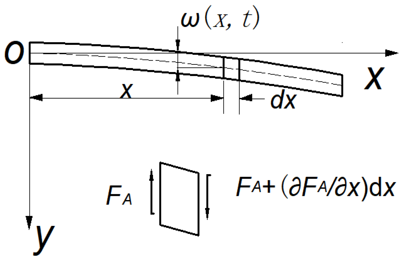
Figure 4.
Model diagram of the DLLFP.
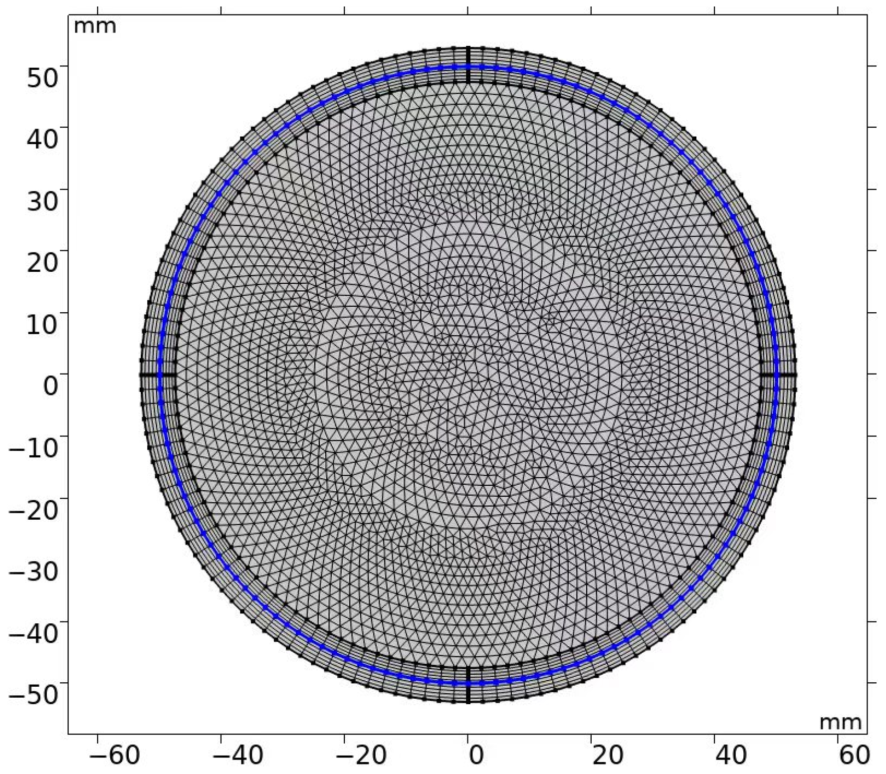
Figure 5.
Comparison of numerical solutions and analytical solutions. (a) Pressure acoustic domain. (b) Solid mechanics domain. (c) Acoustic–structural coupling domain.
Figure 5.
Comparison of numerical solutions and analytical solutions. (a) Pressure acoustic domain. (b) Solid mechanics domain. (c) Acoustic–structural coupling domain.
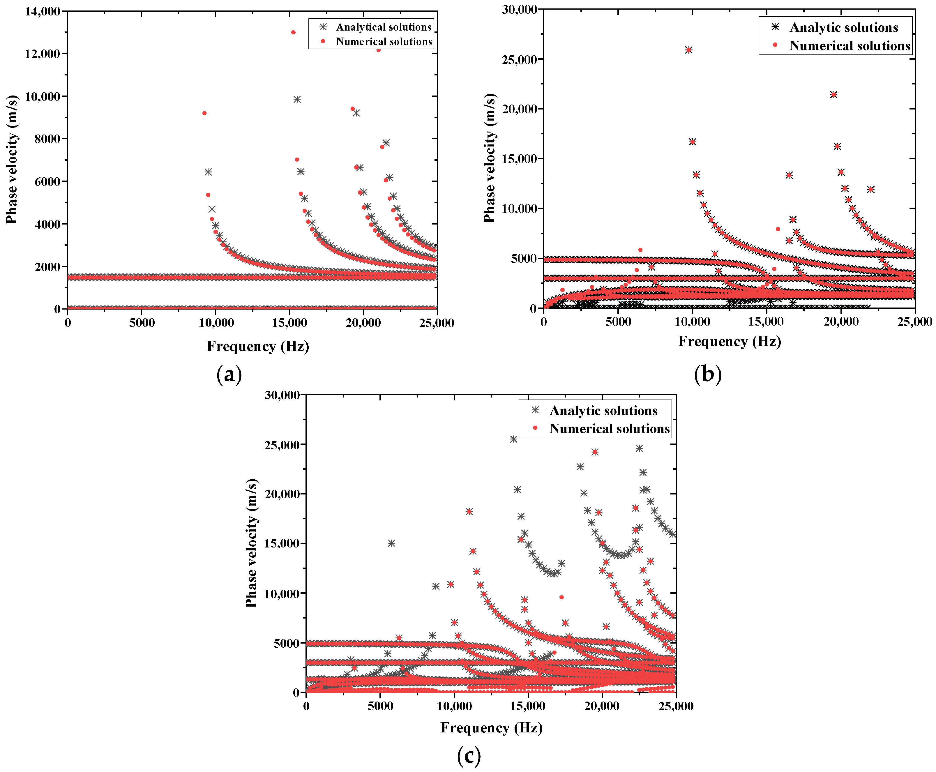
Figure 6.
Sound–structural coupling frequency dispersion diagram.

Figure 7.
Relationship between wavenumber–thickness product and angular frequency of DLLFP. (a) Pressure acoustic domain. (b) Solid mechanics domain. (c) Acoustic–structural coupling domain.
Figure 7.
Relationship between wavenumber–thickness product and angular frequency of DLLFP. (a) Pressure acoustic domain. (b) Solid mechanics domain. (c) Acoustic–structural coupling domain.
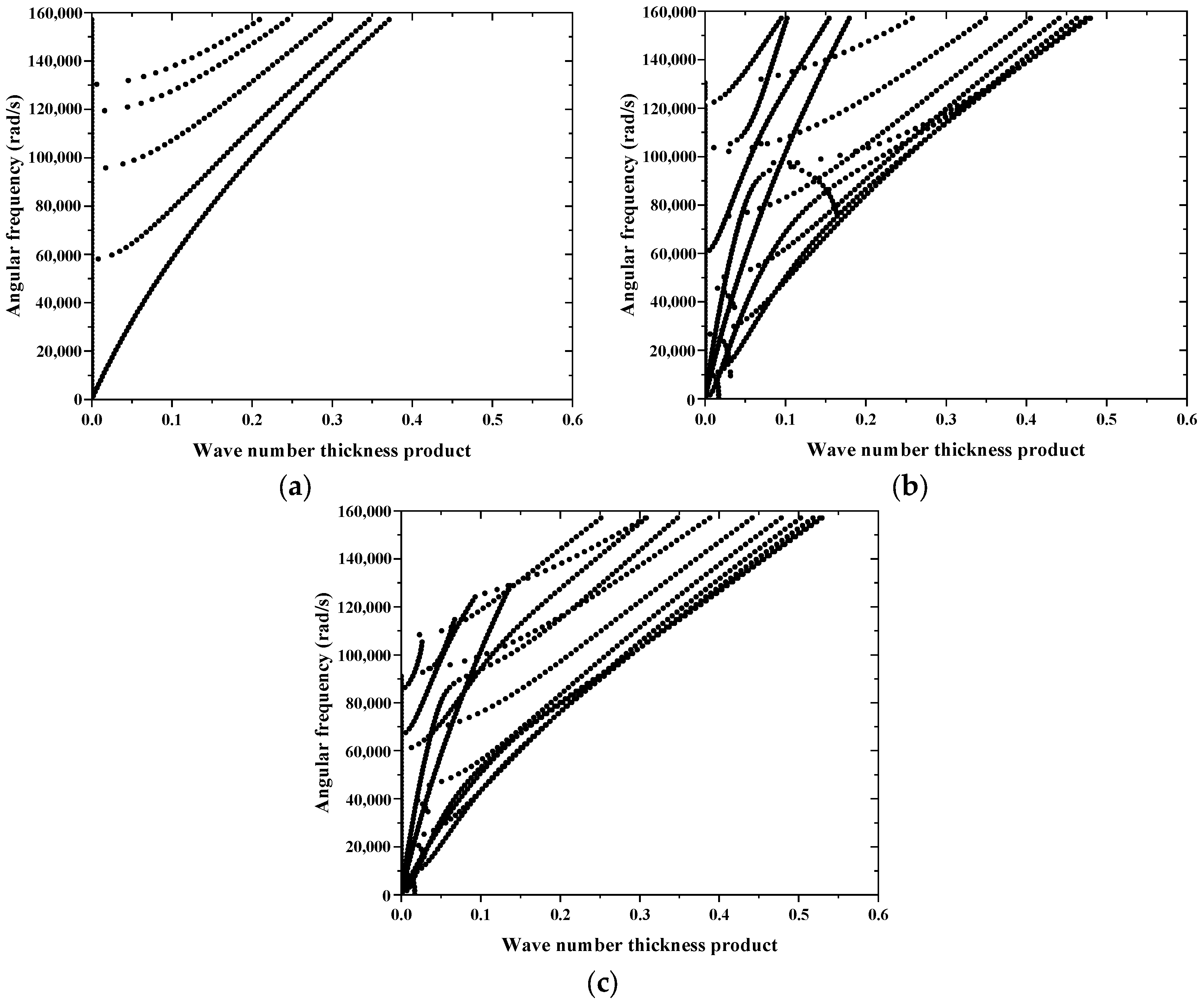
Figure 8.
Absolute sound pressure and stress cloud of a pipeline. (a) f = 5008 Hz k = 10.619. (b) f = 12,755 Hz k = 9.7833. (c) f = 20,752 Hz k = 45.47. (d) f = 20,002 Hz k = 41.412. (e) f = 20,002 Hz k = 60.411. (f) f = 13,505 Hz k = 20.353.
Figure 8.
Absolute sound pressure and stress cloud of a pipeline. (a) f = 5008 Hz k = 10.619. (b) f = 12,755 Hz k = 9.7833. (c) f = 20,752 Hz k = 45.47. (d) f = 20,002 Hz k = 41.412. (e) f = 20,002 Hz k = 60.411. (f) f = 13,505 Hz k = 20.353.


Table 1.
Material parameters.
| Materials | Wall Thickness [mm] | Density ρ [kg/m3] | Sound Velocity c [m/s] | Young’s Modulus E [pa] | Poisson’s Ratio μ |
|---|---|---|---|---|---|
| Structural steel | 2.5 | 7850 | Disregard | 205 × 109 | 0.30 |
| Titanium beta-21Sl | 3 | 4940 | Disregard | 105× 109 | 0.33 |
| Water | Disregard | 1000 | 1500 | Disregard | Disregard |
Disclaimer/Publisher’s Note: The statements, opinions and data contained in all publications are solely those of the individual author(s) and contributor(s) and not of MDPI and/or the editor(s). MDPI and/or the editor(s) disclaim responsibility for any injury to people or property resulting from any ideas, methods, instructions or products referred to in the content. |
© 2023 by the authors. Licensee MDPI, Basel, Switzerland. This article is an open access article distributed under the terms and conditions of the Creative Commons Attribution (CC BY) license (https://creativecommons.org/licenses/by/4.0/).
Share and Cite
MDPI and ACS Style
Yan, J.; Li, J.; Zou, L.; Zhang, D.; Wang, C.; Tang, Z. Acoustic Characteristics Analysis of Double-Layer Liquid-Filled Pipes Based on Acoustic–Solid Coupling Theory. Appl. Sci. 2023, 13, 11017. https://doi.org/10.3390/app131911017
AMA Style
Yan J, Li J, Zou L, Zhang D, Wang C, Tang Z. Acoustic Characteristics Analysis of Double-Layer Liquid-Filled Pipes Based on Acoustic–Solid Coupling Theory. Applied Sciences. 2023; 13(19):11017. https://doi.org/10.3390/app131911017
Chicago/Turabian StyleYan, Jin, Jiangfeng Li, Lvlong Zou, Dapeng Zhang, Cheng Wang, and Zhi Tang. 2023. "Acoustic Characteristics Analysis of Double-Layer Liquid-Filled Pipes Based on Acoustic–Solid Coupling Theory" Applied Sciences 13, no. 19: 11017. https://doi.org/10.3390/app131911017
Note that from the first issue of 2016, this journal uses article numbers instead of page numbers. See further details here.