

Design Optimization of a Hydrodynamic Brake with an Electrorheological Fluid

1
Faculty of Mechanical Engineering, Kazimierz Pulaski University of Technology and Humanities in Radom, 26-600 Radom, Poland
2
Branch in Sandomierz, Jan Kochanowski University of Kielce, 25-369 Kielce, Poland
3
Department of Mechanical Engineering, The State University of New York, (SUNY Korea), 119 Songdo Moonhwa-Ro, Yeonsu-Gu, Incheon 21985, Republic of Korea
4
Department of Mechanical Engineering, Industrial University of Ho Chi Minh City (IUH), 12 Nguyen Van Bao Street, Go Vap District, Ho Chi Minh City 70000, Vietnam
*
Author to whom correspondence should be addressed.
Appl. Sci. 2023, 13(2), 1089; https://doi.org/10.3390/app13021089
Submission received: 5 December 2022
/
Revised: 5 January 2023
/
Accepted: 10 January 2023
/
Published: 13 January 2023
(This article belongs to the Special Issue Magneto-Rheological Fluids)
Abstract
:This article describes the design optimization of a hydrodynamic brake with an electrorheological fluid. The design optimization is performed on the basis of mathematical model of the brake geometry and the brake’s electrical circuit. The parameters of the mathematical models are selected based on experimental tests of the prototype brake. Six different objective functions are minimized during the design optimization. The functions are created taking into consideration the following factors: the braking torque, brake weight, electric power absorbed by the brake, and the torque rise time. The assumed design variables are: the number of blades and the radii (inner and outer) of the brake’s working space. The optimization calculations are performed for two design variables intervals. The first interval is defined taking into consideration the accuracy of the mathematical model. The second, narrower interval is assumed for the tested prototypical brake. On the basis of the optimization calculation results, general guidelines are presented for the optimization of the hydrodynamic brakes with an ER fluid. In addition, the possibilities of optimizing the prototype brake are determined.
1. Introduction
Hydrodynamic brakes (HB) belong to the group of hydraulic components of machines, as do clutches and hydrodynamic torque converters. They are used in drive systems of machines, mainly due to their favorable weight-to-torque ratio on the input shaft and the long durability [1]. The basic way of controlling the HBs is by changing their working fluid filling degree. The lower the filling degree, the smaller the torque on the input shaft of the brake. However, the dependence of the torque on the filling degree is not linear. Moreover, this manner of control has a significant disadvantage, which is the unstable operation of HB at low filling degrees. The analysis of the operation of hydrodynamic components leads to the conclusion that controlling them is also possible by changing properties of the working fluid [2]. Thus, in this case, it is possible to use smart fluids, which react with a change in shear stress when exposed to changes in the electrical field (electrorheological fluids) or in the magnetic field (magnetorheological fluids) [3,4]. Currently, smart fluids are used in numerous devices and components of machines, e.g., in viscous clutches and brakes [5,6,7], shock absorbers [8,9,10], valves [11,12,13], sealings [14], cantilever sandwich beams [15,16], landing gear systems in planes [17,18], and industrial robots [19,20,21]. In addition, prototypes of hydrodynamic clutches with electrorheological fluids (ER) and magnetorheological fluids (MR) are constructed [22,23,24,25].
A frequent method of perfecting the design of machine components is the use of construction optimization. The construction optimization is performed on the basis of the component’s mathematical model. The model parameters whose values are changed during the optimization process are called the design variables. The objective function is determined, and then its global extreme is sought on the basis of the requirements analysis assigned to the machine component (i.e., criteria) and to the mathematical model. To search for the global extreme of the objective function, multiple methods have been developed. Among the most frequently used methods are randomization methods, including the Monte Carlo Method and the Genetic Algorithm method [26,27,28]. It is advantageous to use structure optimization methods in the design process due to the complex design of hydraulic clutches with ER or MR fluids, which results from the necessity to generate an electric field inside. For mathematical modeling of clutches, brakes and torque converters, and one-, two-, and three-dimensional flows within the rotors are taken into consideration [29,30,31]. In the model based on the one-dimensional flow, it is assumed that the working fluid moves with the mean flow path with a uniform through-flow velocity [32]. The high accuracy of this model, comparable to the accuracy of two- and three-dimensional models, is obtained as a result of parameter selection based on experimental research. Due to their simplicity, these models are particularly suitable for use in design optimization [33].
Publications concerning the optimization of brakes and hydraulic clutches with smart fluids most frequently concern viscous clutches and brakes with MR fluids [34,35]. The article [36] describes the design optimization of a disc viscous clutch with ER fluids. The optimization is performed with the use of two optimization methods: the Monte Carlo method and the Genetic Algorithm method. The purpose of the design optimization is to seek such values of design variables, for which the viscous clutch with the ER fluid transmits a large torque, while the clutch’s dimensions are small and its determined operating temperature is low. The optimization calculations are performed for two models including three and eight design variables. As a result of the design optimization, a disc viscous clutch with the ER fluid is constructed. In the publication [37], the object of the optimization process is a disc brake with a MR fluid. The brake was intended for use in a motorcycle. The objective function is the brake’s weight, and the assumed constraints of the design variables are the braking torque and the temperature of the MR fluid during braking. The optimization is performed with the use of optimization procedures from the ANSYS program. In the article [38] the optimized object is a disc brake with one disc and different locations of the electromagnet coils and with three types of MR fluid. The constraints of the design variables concern the radius of the brake shaft and the maximal current flowing through the electromagnet coil. The optimization is conducted on the basis of the optimization method included in the ANSYS software. In the objective functions, factors taken into consideration are the brake’s weight, the power supply, and the braking torque. The work [39] shows the use of an original Taguchi method in the optimization of a clutch with a MR fluid. The method allows identification of decision variables whose influence on the objective functions is the greatest.
Apart from the use for hydraulic clutches and brakes with ER fluids, design optimization has also been successfully used to optimize devices with smart fluids [11,40]. Despite several works on design optimization for ER brakes or MR brakes, a study on the optimal design of ER brakes considering practical feasibility, in which many design parameters should be considered, is considerably rare. Thus, in this work, to achieve this target, many principal design parameters, such as the radius and electrode gap of ER brake, and several braking performance and product criteria also, such as torque level, blade number, brake weight, electric power and braking time, are included for the optimization. To accomplish such a target, the HB optimization method is used, and subsequently, the possibilities of optimal selection of considered parameters of the optimized prototypical hydrodynamic brake with the ER fluid (PHB) are discussed in detail, focusing on the performance efficiency with several ratios: the blade number versus torque level versus brake weight. Consequently, the main technical contribution of this work is to calculate the optimized design and performance variables of the PHB that can be feasible in a practical environment. As far as the authors know, so far there is no report on this optimal design issue in the technology associated with ER fluid systems, such as hydrodynamic brakes.
2. Construction of the Hydrodynamic Brake
The HB has rotors with radial blades lying in planes passing through the rotor axis. These rotors have no inner rings. Such a design solution is frequently used in practice. The construction scheme of the HB is shown in Figure 1.
The HB is filled with the ER fluid. The pump rotor rotates with the angular velocity ω1, and the turbine rotor is immobile (ω2 = 0). The meridional cross-sections of both HB rotors are identical. The casing and rotors are made of an electrical insulator material, while the blades are made of an electrical conductor material. The pump and turbine blades are alternately connected to the (+) and (−) poles of the high voltage power supply with the use of slip rings, brushes, and electric wires. The HB operates as follows: the rotating pump rotor sets the fluid in motion; the fluid then flows into the immobile turbine rotor and presses on the blades, which causes the reaction torque to occur. After supplying the high voltage U to the rotor blades, the electric field is created, and it causes an increase in the shear stresses τ within the ER fluid. This causes an increase in the fluid flow resistance and, simultaneously, a decrease in the torque M affecting the pump rotor. Thus, the HB operates differently than a viscous brake with an ER fluid, in which an increase of the high voltage U causes an increase in the torque. The designations of the basic dimensions of the HB are shown in Figure 2.
The following notations are used in Figure 2: R—the outer radius of the rotors, rw—the inner radius of the rotors, n—the number of blades, gb—the blade thickness, d1—the smallest distance between blades, d2—the largest distance between blades, rs—radius, determining the origin of the mean streamline, r1—the inner radius of the mean streamline, r2—the outer radius of the mean streamline, ω1—angular velocity of the pump rotor, ω2—angular velocity of the turbine rotor. The design solution for PHB is shown in Figure 3.
The PHB rotors are made of 3D-printed nylon. They are equipped with flat steel sheet blades. The basic data concerning the PHB are shown in Table 1.
3. The Mathematical Model of the Hydrodynamic Brake
3.1. The Mathematical Model of the Hydrodynamic Brake Geometry
The parameters describing the geometry of the brake rotors are as follows: the outer radius of the rotors R, the inner radius of the rotors rw, and the number of blades n. The radius R is larger than the radius rw. The blade number n is even, so that in each of the channels formed by the blades, an electric field influences the ER fluid. Moreover, the blades cannot be set too close to each other due to the possibility of electric breakdown occurrence. Thus, the number of the blades should meet the following condition:
where gb—blade thickness, hmin—the smallest gap width for which an electric breakdown occurs. The average blade distance d is calculated from the formula:
wherein:
where d1—the smallest distance between blades, rw—inner radius of the rotors, R—outer radius of the rotors, d2—the largest distance between blades, n—number of blades.
In order to calculate the rotor volume Vt, the following formula is used:
where R—outer radius of the rotors, rw—inner radius of the rotors.
The blades volume Vb is calculated on the basis of the following formula:
where n—number of blades, rw—inner radius of the rotors, R—outer radius of the rotors, gb—blade thickness.
The volume of the fluid VER contained in the HB is then:
where Vt—the rotor volume, Vb—the blades volume. With the use of the Formulas (4)–(6), it is possible to formulate the weight G of the brake as follows:
where ρ—density of the working fluid, ρ1—density of the blade material, ρ2—density of the casing material, α—coefficient describing the casing density in relation to the rotor volume.
3.2. Mathematical Model of Hydraulic Interactions
In order to calculate the transferred torque M, the one-dimensional flow model of a hydrodynamic clutch is used [41,42]. The torque M for the HB is obtained from the equations of the one-dimensional flow model of a hydrodynamic clutch after assuming that ω2 = 0. It is assumed that the flow of the working fluid inside the hydrodynamic clutch is steady, continuous, and takes place along a single line of the mean stream. The radii r1, r2, rs (Figure 3) determining the position of the mean streamline in the meridional cross-section are calculated on the basis of the following formulas:
where rw—inner radius of the rotors, R—outer radius of the rotors. The unit torque dM in relations to the rotation axis of the rotor is only caused by the force dF caused by a change in speed cu of the working fluid particles. The force dF and the unit torque dM are written as:
where d/dt—differential operator, t—time, m—mass of the fluid particle, cu—lifting speed, r—radius. The mass m of the fluid flowing over time dt can be calculated as:
where V—fluid volume, t—time, Q—flow rate, cm—meridional speed, A—rotor meridional cross-section. After taking into consideration the dependence (11) in relation to (10), the following is obtained:
where the product cur is treated as a single variable. Integrating the dependence (12) from point 1 to point 2 positioned on the mean streamline leads to the following equation:
where ρ—density of the working fluid, Q—flow rate, cu—lifting speed, r—radius.
When the blades of the hydrodynamic clutch are positioned in the planes passing through the rotor axes, then the rotor lifting speed is, respectively:
where ω1—angular velocity of the pump rotor, ω2—angular velocity of the turbine rotor, r1—the inner radius of the mean streamline, r2—the outer radius of the mean streamline. For the determined operation conditions of the hydrodynamic clutch:
where cm—meridional speed, A—rotor flow field. Considering the fact that for the HB, the angular velocity of the clutch turbine rotor ω2 equals zero, on the basis of dependences (13)–(15), the following is obtained:
where ρ—working fluid density, cm—meridional speed, A—rotor flow field, ω1—angular velocity of the clutch pump rotor. After taking into consideration the blade thickness, the flow field of the HB is:
where n—number of blades, gb—blade thickness. In order to calculate the meridional speed cm, the head rise balance is considered, described as:
where Δp—pressure change, ρ—working fluid density, g—gravitational acceleration. The balance of the head rise has the following form:
where h1—head rise of the pump, hu—impact loss, ht—friction loss. For HBs with typical working fluids, the components of Equation (19) are written as follows:
where ω1—angular velocity of the pump rotor, g—gravitational acceleration cm—meridional speed, r1—the inner radius of the mean streamline, r2—the outer radius of the mean streamline, ξ—friction losses factor.
During the HB modeling, in the presence of an electrical field, when considering the friction losses value ht (described with Formula (22), it is necessary to take into account the decrease in pressure ΔpER caused by the increase in the shear stresses τ. On the basis of the formulas used for calculation of the valves with ER fluids [11,12,13,43,44], it is assumed that:
where c—numerical coefficient, l—length of the channel formed by the blades, d—average distance between blades, τ0—yield stress. After taking into consideration Formula (23) in Formula (18), and subsequently adding the result to Formula (22), the following is obtained:
where ξ—friction losses factor, cm—meridional speed, g—gravitational acceleration, r1—the inner radius of the mean streamline, r2—the outer radius of the mean streamline, c—numerical coefficient, l—length of the channel formed by the blades, τ0—yield stress, d—average distance between blades. The meridional speed cm, which enables the calculation of the torque M on the basis of Formula (16), is obtained by substituting Formulas (20), (21), and (24) to the equation for the head rise balance (19) and subsequently solving the equation:
wherein:
where ω1—angular velocity of the pump rotor, r1—the inner radius of the mean streamline, r2—the outer radius of the mean streamline, τ0—yield stress, ξ—friction loss coefficient, ς—channel coefficient, c—numerical coefficient, l—length of the channel formed by the blades, ρ—density of the working fluid, d—average distance between blades.
3.3. Mathematical Model of the Electric Circuit of the Hydrodynamic Brake
Electrorheological properties of the ER fluids are presented with the use of the following formulas:
wherein:
where τ0—yield stress, ig—leakage current density, a, b—coefficients, E—the electric field intensity, U—voltage, d—average distance between blades. The dependence of τ0 and ig on the temperature Θ is not taken into account, because it is assumed that the HB operates at a constant temperature due to the use of a cooling system. The HB needs to be cooled, because all the energy supplied to the HB is converted to heat. The leakage current flowing between the electrodes is calculated on the basis of the formula:
wherein:
where Se—surface of the electrodes, n—number of blades, rw—inner radius of the rotors, R—outer radius of the rotors.
In the considered model, the increase of the high voltage U applied to the blades causes a decrease in the meridional speed cm until it reaches zero. The meridional speed cm is described by Formula (25). The value of the voltage Uh for which cm= 0 can be calculated on the basis of the equation:
where ω1—angular velocity of the pump rotor, r1—the inner radius of the mean streamline, r2—the outer radius of the mean streamline, ς—channel coefficient, τ0—yield stress. Having taken into consideration Formulas (27) and (29) in Equation (32), the following is obtained:
where ω1—angular velocity of the pump rotor, r1—the inner radius of the mean streamline, r2—the outer radius of the mean streamline, a, c—coefficients, l—length of the channel formed by the blades, ρ—working fluid density, d—average distance between blades. The maximal power Pe obtained from the power supply, while stopping the flow of the ER fluid in the brake, is:
where Uh—voltage value for which cm= 0, icmax—leakage current calculated for U = Uh.
In order to assess the dynamics of the HB, the torque rise time M (after applying the high voltage to the electrodes Uh) is taken into consideration. The dynamics of the machine drive system containing the HB is not taken into account due to the fact that the total mass moment of inertia on the input shaft depends not only on the HB structure, but also on the structure of the drive system. The drive system structure, due to the general nature of the considerations, is not specified. The torque rise time for the HB are considered on the basis of the voltage courses in a simplified electrical circuit of the HB, as shown in Figure 4 [45].
The blades of the HB, separated from each other by the ER fluid, form a capacitor whose capacity is Ce. The ER fluid provides the electrical resistance Re during the leakage current flow ic. After applying the supply voltage U1, the electric current flows through the wires (the resistance of the wires is re) to the condenser with the capacity of Ce and charges the condenser. After the power supply U1 is switched off, the electric current flows through the ER fluid whose resistance is Re, and the condenser discharges. Changes of the voltage U2 over time, with a step voltage increase U1, is described by a first order system. It is assumed that the torque of the HB does not depend on time, but it is proportional to the voltage U2. While the condenser is charging, the time constant of the first order system is Tc = re·Ce, whereas while the condenser discharges, it is Td = Re·Ce. Due to the fact that re<<Re, Td>>Tc, the operation speed of the HB is assessed with the use of the time T described with the formula:
wherein:
where β—number of time constants after which U1≅U2, Uh—value of the voltage for which cm= 0, icmax—leakage current calculated for U = Uh, ε0—electric permittivity of the vacuum, εr—relative permittivity of the ER fluid, Se—surface of the electrodes, d—average distance between blades.
3.4. Coefficient Selection for the Mathematical Model of the Hydrodynamic Brake
Before using the developed HB model in optimization calculations, it is necessary to determine the values of the model’s coefficients: α, ξ, c, a, b, β, εr. The values of the coefficients are determined on the basis of the design analysis and PHB experimental research. The coefficient α is calculated on the basis of the PHB weight, assuming that the modelled HB has an identical structure and proportional dimensions. Calculating the coefficient ξ demanded PHB bench tests without connecting the blades to the high voltage power supply. The test bench scheme is shown in Figure 5.
The main elements of the test bench are: an electric drive motor and a torque gauge. The computer control system of the test bench rendered it possible to obtain the measurement values specified in the test program, as well as to collect and process measurement data. The values recorded during the test are: the angular velocity of the pump shaft ω1, the braking torque M, and the temperature of the working fluid Θ. The temperature Θ is maintained at 35 °C by cooling the PHB with compressed air. Subsequently, the braking torque M is measured at a predetermined angular velocity of the PHB input shaft. The coefficient ξis determined on the basis of Formulas (14) and (23). During the measurement, apart from the braking torque M, the rotational torques are of resistance to motion of the bearings and sealing. In further considerations, the torques of resistance are omitted due to their low values [42]. The value of the a coefficient is determined on the basis of the data from the manufacturer of the fluid LID3354S [46].
In order to determine the coefficient c for the immobile turbine shaft and for a specified angular velocity of the pump shaft ω1, the braking torque M of the PHB is measured for a few selected voltages U. To generate the high voltage U, an electric power supply with a rated power of 18W is used. The maximal voltage U obtained during these measurements is Umax = 3 kV. The coefficient c is selected, so that for the voltage Umax = 3 kV, the torque calculated with the use of the dependence (22) is equal to the torque measured with the use of the test bench, i.e., M = 1.733 Nm, Figure 6.
The coefficient b is selected in order to obtain the measured total leakage current ic = 6 mA for the voltage U = 3 kV. The value of the relative electric permittivity εr of the ER fluid is determined on the basis of [47,48]. The coefficient values of the HB mathematical model determined for ω1= 200 rad/s and for the temperature Θ = 35 °C are presented in Table 2.
Due to the chosen method of selecting the coefficients shown in Table 2, only the modelling error of the dependence of the torque M on the high voltage U can be assessed. The solid line shown in Figure 6, obtained on the basis of the mathematical model, according to the assumptions, passes through the points for U = 0 kV and U = 3 kV. The average relative error calculated for U = 1 kV and U = 2 kV is under 2%.
4. Optimization Method for the Hydrodynamic Brake Design
In order to obtain guidelines for optimization of the HB design (concerning the selection of design variables and objective functions), calculations are performed on the basis of the developed mathematical model. Two calculation groups are performed. One group includes the detailed PHB calculations, on the basis of which the design variables are selected. The other group contains the general HB calculations, on the basis of which the optimization criteria are selected. For the HB, the calculation data are randomly selected parameters from determined ranges.
4.1. Selection of Design Variables
The calculations for the PHB are performed for the data shown in Table 1. The torque M and the voltage Uh are calculated, while one of the parameters rw, R, n is changed, and the remaining parameters are fixed. Examples of the calculation results for ω1 = 200 rad/s, Θ = 35 °C are shown in Figure 7, Figure 8 and Figure 9.
Figure 7 presents the influence of the radius rw and the radius Ron the braking torque M. Figure 8 shows the dependence of the braking torque M on the blade number n. Figure 9 shows the influence that the number of blades nin the PHB has on the value of the voltage Uh. As shown in Figure 7, increasing the inner radius rw causes a decrease in the braking torque M, while increasing the outer radius R causes an increase in the torque M. This is related to the opposing influence of these radii on the flow velocity of the ER fluid within the rotors. Increasing the blade number n, Figure 8, causes a decrease in the torque M, which is connected to the decrease of the flow cross-sectional area A of the rotors. Figure 9 shows a decrease in voltage Uh as the number of blades increase, with a constant value of the torque M. The decrease is a result of decreasing average distance between blades d when the number of the blades increases. Decreasing the value of d causes an increase in the electric field strength E, which has a direct influence on the value of the yield stresses τ0. A significant (and different) influence of the radii rw and R, as well as the number of blades n, on the PHB characteristics justifies the purposefulness of selecting these parameters as design variables for optimization of the PHB design.
4.2. Selection of Optimization Criteria
The calculations included the dependence of weight G, electric power Pe, and time T on the torque M, as well as the dependence of the torque M, weight G, electric power Pe, and time T on the radii rw, R, and the blade number n. The intervals of the HB parameters and additional conditions ensuring the absence of electric breakdowns are shown in Table 3.
The HB parameter intervals are determined arbitrarily, aiming at possibly small differences between the parameters of the calculated HB and the parameters of the PHB used to determine the coefficients of the mathematical model. This allows obtaining the necessary accuracy of the used mathematical model. The HB calculations are performed as follows:
- it is assumed that ω1 = 200 rad/s;
- the radii rw and R are randomly selected from the intervals given in Table 3;
- it is assumed that gb = 0.02 R;
- calculations are performed according to the formulas of the mathematical model described in Section 2;
- the calculation results not meeting the requirements given in Table 3 are rejected.
The calculations are performed on the basis of a computer program written in Turbo Pascal 7. Examples of calculation results for 5000 draws and for ω1= 200 rad/s and Θ = 35 °C are shown in Figure 10, Figure 11, Figure 12, Figure 13, Figure 14, Figure 15, Figure 16, Figure 17 and Figure 18.
Figure 10 and Figure 11 show the proportional dependence of the weight G and electric power Pe on the torque M. Different values of the weight G and the power Pe occurring for the same values of the torque M are mostly a result of the difference in the number of blades n. For fixed values of the radius rw and the radius R, the smaller the number of blades n, the smaller the weight G. In this case, the dependence of the power Pe on the number of blades is the opposite; the smaller the number of blades n, the higher the voltage Uh necessary to reach the yield stress τ0 needed to stop the flow of the ER fluid (and, therefore, the power Pe is greater). Figure 12 shows that small values of time T occur for all values of the torque M. A wider range of the time values T for smaller torques M is a result of smaller dimensions of the HB and, therefore, smaller distances between blades and a larger capacity Ce. As shown in Figure 13 and Figure 14, the dependence of the torque M and the electric power Pe on the number of blades are similar. The largest values of M and Pe occur within the range from n = 30 to n = 40. The increase of the average time values T with the increase in the number of blades n can be observed in Figure 15. It is a result of the smaller distances between blades and, therefore, larger capacities Ce on which the time T depends. As shown in Figure 16 and Figure 17, the dependence of the torque M and the electric power Pe on the radius rw and on the radius R are similar. As can be seen in Figure 18, by changing the value of the radius rw and the radius R in the intervals presented in Table 3, one can obtain similar values of time T.
The dependences of weight G, electric power Pe, and time T on the torque M are not functions; thus, HBs with the same value of the torque M can have different weights G, electric powers Pe, and times T. Moreover, M, G, Pe, and T significantly (and in different ways) depend on the assumed design variables rw, R, and n. Due to that, the torque M, weight G, electric power Pe, and time Ts are selected as optimization criteria for the design and are used to formulate the objective functions F. The selection of the criteria is consistent with the pursuit of mechanical engineering to increase efficiency, reduce weight, and save energy. The requirements concerning the assumed design optimization criteria are presented in Table 4.
4.3. The Algorithm for Design Optimization of the Hydrodynamic Brake
The objective functions FG, FP, FT,FG1, FP1, FT1 described by Formulas (38)–(40) cannot be written using simple formulas, in which there are the design variables, due to the complicated form of the applied mathematical model. The values of the criteria G, M, Pe, T were calculated on the basis of the formulas given in Table 4. The numerical coefficients appearing in the Formulas (38)–(40) are arbitrarily selected during initial calculations, so that minimal values of the objective functions FGmin, FPmin, FTmin are as close to zero as possible. The objective function, which is the difference between G and M, is also assumed in the articles [49,50]. The minimalization of the objective functions (38)–(40) leads to finding the design variables, for which the unit of the torque M will be assigned with, respectively, the lowest weight G, the lowest electrical power Pe, and the shortest time T. The design variables intervals rw, R, n and constraints concerning d1 and Uh are the ones given in Table 3. The optimization calculations for the HB are aimed at minimizing the selected objective function F described with one of the Formulas (38)–(40).The calculations are performed as follows:
- the decision variables rw, R, and n are randomly selected from the assumed intervals with the use of a random number generator;
- the value of ω1 is determined and gb = 0.02R is calculated;
- calculations are performed according to the formulas of the mathematical model;
- the constraints of d1 and Uh are checked;
- when the randomly selected values of the design variables meet the conditions of the constraints, the objective function F is calculated, its result is saved, and the calculations are repeated;
- the smaller value of the objective function from the previous Fp and present step of the calculations Fa is selected;
- the values of the design variables rw, R, and n are saved, and on the basis of these values, an objective function of a smaller value is obtained.
The scheme of calculations carried out in one calculation step of a computer program is shown in Figure 19.
5. Design Optimization Results and Discussion
The results of the calculations shown in Figure 10, Figure 11 and Figure 12 demonstrate that it is not possible to determine intervals of the torque M, for which there are minima of the considered objective functions. Due to that, initially, the design optimization of the HB is carried out for the entire range of decision variables. The results of the HB design optimization for 150,000 draws are shown in Table 5. The placement of the minima Fmin of the objective function F on the background of the “Pareto chart” showing the dependence of the “lightness of construction” (described as 1/G) on the torque M is depicted in Figure 20. Table 6 contains the values of the ratios: G/M, Pe/M, T/M and G, Pe, T calculated on the basis of the data from Table 1. In order to assess the possibility of PHB optimization, calculations are made with the assumption that the braking torque M meets the requirement 1.700 Nm <M < 1.800 Nm, i.e., it is close to the torque of the experimentally tested PHB: M = 1.733 Nm. Assuming such a small range of torque M variations increases the possibility of finding the minima of the objective functions. A few percent change of the torque M during the HB selection for a machine’s drive system is acceptable. Table 7 shows the results of these calculations for 150,000 draws. It is justified to assume the quotients of the criteria listed in Table 4 as the functions of the objectives, because the quotients G/M, Pe/M, T/M can be interpreted as efficiency related to 1 Nm. For instance, G/M = 0.497 kg/Nm means that 1 Nm of the braking torque M corresponds to 0.497 kg of the HB mass. Table 5 shows that the minimum of the objective function is achieved for torques M of approximately 7.5 Nm for the objective functions FG, FG1; 0.2 Nm for the objective functions FPe, FPe1; and 9.9 Nm for the objective functions FT, FT1. Therefore, the HBs having a large braking torque M have a low G/M ratio and a low T/M ratio, which is advantageous. On the contrary, the HBs having a low braking torque M have unfavorable values of G/M ratio and especially T/M ratio, but the value of the Pe/M ratio is advantageous. The minimal value of the G/M ratio does not correspond to the minimal value of the HB, due to the large differences between the values of the torques. However, the minimal values of the Pe/M and T/M ratios occur for the minimal values, respectively, Pe and T. Proximate values of the G/M, Pe/M, T/M ratios, defined for the objective functions as differences and quotients of criteria, prove the correctness of the performed calculations. Table 6 and Figure 20 show that the PHB is not an optimal brake in terms of the considered criteria. This is proven by the high values of the G/M, Pe/M, T/M ratios, as well as the placement of point 7 beyond the “Pareto front” (which is a set of points with the lowest values of 1/G). Table 7 shows that the minimal values of the G/M, Pe/M, and T/M ratios occur for the minimal values of, respectively, G, Pe, and T. The optimized PHBs with a lower weight also have lower mass moments of inertia. This results in the fact that these brakes have a short head rise time of the torque M. Table 7 also shows that the values of the braking torque M, differing from each other by less than 4%, are obtained for significantly different values of design variables. The relative differences between the highest and lowest values of individual design variables, related to the average values, are 80% for rw, 12% for R, and 83% for n. Whereas, the relative differences between the highest and lowest values of the ratios G/M, Pe/M, and T/M are respectively 54%, 140%, and 146%.
The initial values of PHB presented in Table 6 can be compared with the optimized values presented in Table 7. The comparison of the values of the G/M, Pe/M and T/M ratios (presented in Table 6 and Table 7) show that, on the basis of the design optimization, it is possible to reduce the following factors: the weight of PHB 1.7 times, the maximum electric power 1.5 times, and the time T 2.5 times. However, these benefits cannot be gained simultaneously. The results shown in Table 7 confirm that it is advisable to improve the PHB design on the basis of design optimization methods. Due to the fact that the selection of decision variables is random, repeating the optimization calculation always provides different results. Moreover, it is not possible to unequivocally determine the optimal number of draws because there is always a possibility that the following draws will provide better results. However, it is necessary to take into consideration the fact that, during the design optimization, only the changes of radii rw and R by tenths of a millimeter are practically significant.
6. Conclusions
On the basis of the performed optimization calculations concerning the design of the HB with the ER fluid, the following conclusions have been achieved:
- Performing the optimization of the HB with the ER fluid requires formulating a mathematical model, establishing constraints, and selecting design variables and the objective function. While planning the design optimization, it is advisable to aim at a simple mathematical model and a low number of design variables, especially when the optimization calculations are performed with the use of the Monte Carlo method (so that it is possible to perform a large number of calculations within an acceptable time). On the basis of the obtained results of the optimization of the HB with the ER fluid, it can be presumed that the assumptions are correct.
- The form of the objective function has a significant influence on the optimization results. However, there are no strict rules as to how the objective function should be formulated. This is why the selection of the objective function is always arbitrary. It is advisable to formulate the objective function in a simple way, so that the results of optimization calculations are easy to interpret. Defining two different objective functions on the basis of the same criteria increases the probability of finding the optimal solution. Due to that, it is justifiable to use the difference and quotient of only two criteria when optimizing the design of the HB with the ER fluid in order to determine the objective function.
- The Monte Carlo method can be successfully used for design optimization of brakes with ER fluid for three design variables. Increasing the number of the design variables causes an exponential increase in the number of draws necessary to obtain the required accuracy of calculations. Not all optimization methods can be used for this purpose because the number of blades, which is a natural number, causes the calculations to be discrete.
- In order to obtain credible and reliable results of the optimization calculations, it is advisable to select coefficients for the assumed mathematical model, as well as for the range of the mathematical model. It is especially important when the HB optimization calculations are performed with the use of a mean streamline model whose accuracy depends on the correctness of the selected coefficients.
It is finally remarked that the optimized method proposed based on the mathematical model can be used when the design of the transmission system is specified only. Therefore, it is a general optimization method that can be applied to optimally design several application systems utilizing ER fluid and MR fluid also.
Author Contributions
I.M. and Z.K. contributed conception and design of the study. Z.K. conducted optimization analysis and calculations. Z.K. and I.M. carried out tests. Z.K. and I.M. wrote the first draft of the manuscript. S.-B.C. contributed to idea analysis, manuscript revision, reading, and approving the submitted version. All authors have read and agreed to the published version of the manuscript.
Funding
The authors received no external funding.
Institutional Review Board Statement
Not applicable.
Informed Consent Statement
Not applicable.
Data Availability Statement
Not applicable.
Conflicts of Interest
The authors declare no potential conflict of interest with respect to the research, authorship, and publication of this article.
References
- Brun, K.; Meyenberg, C.; Thorp, J. Hydrodynamic torque converters for oil & gas compression and pumping applications: Basic principles, performance characteristics and applications. In Proceedings of the Asia & Pump Symposium Marina Bay Sand, Singapore, 22–25 February 2016; pp. 1–15. [Google Scholar] [CrossRef]
- Kęsy, Z.; Kęsy, A. Prospects for the control of a torque converter using magnetic fluid. In Proceedings of the IEEE International Colloquium on Innovative Actuators for Mechatronic Systems, London, UK, 18 October 1995; pp. 10-1–10-3. [Google Scholar]
- Dong, Y.Z.; Seo, Y.; Choi, H.J. Recent development of electro-responsive smart electrorheological fluids. Soft Matter 2019, 15, 3473–3486. [Google Scholar] [CrossRef]
- Qader, I.N.; Kök, M.; Dagdelen, F.; Aydogdu, Y.A. Review of smart materials: Researches and applications. El-Cezeri Fen Ve Mühendislik Derg. 2019, 6, 755–788. [Google Scholar] [CrossRef]
- Bulough, W.; Johnson, A.R.; Tozer, R.; Makin, J. Electrorheological clutch, methodology, performance and problems in ERclutch based positioning mechanisms. Intern. J. Mod. Phys. B13 1999, 14, 2101–2108. [Google Scholar] [CrossRef]
- Li, W.H.; Du, H. Design and experimental evaluation of a magnetorheological brake. Int. J. Adv. Manuf. Technol. 2003, 21, 508–515. [Google Scholar] [CrossRef]
- Choi, S.B.; Cheong, C.C.; Kim, G.W. Feedback control of tension in moving tape using an ER brake actuator. Mechatronics 1997, 7, 53–66. [Google Scholar] [CrossRef]
- Wereley, N.M.; Lindler, J.; Rosenfeld, N.; Choi, Y.T. Biviscous damping behavior in electrorheological shock absorbers. Smart Mater. Struc. 2004, 13, 743–752. [Google Scholar] [CrossRef]
- Choi, S.B. Performance comparison of vehicle suspensions featuring two different electrorheological shock absorbers. Proc. Inst. Mech. Eng. Part D J. Automob. Eng. 2003, 217, 999–1010. [Google Scholar] [CrossRef]
- Gołdasz, J.; Sapiński, B. Insight into Magnetorheological Shock Absorbers; Springer International Publishing: Cham, Switzerland, 2003. [Google Scholar] [CrossRef]
- Rosenfeld, N.C.; Wereley, N.M. Volume-constrained optimization of magnetorheological and electrorheological valves and dampers. Smart Mater. Struc. 2004, 13, 1303–1313. [Google Scholar] [CrossRef]
- Choi, S.B.; Choi, W.Y. Position control of a cylinder using a hydraulic bridge circuit with ER valves. J. Dyn. Syst. Meas. Control 2003, 122, 201–209. [Google Scholar] [CrossRef]
- Kciuk, S.; Martynowicz, P. Special application magnetorheological valve numerical and experimental. Solid State Phenom. 2011, 177, 102–115. [Google Scholar] [CrossRef]
- Szczęch, M. Theoretical analysis and experimental studies on torque friction in magnetic fluid seals. Proc. Inst. Mech. Eng. Part J J. Eng. Tribol. 2020, 234, 274–281. [Google Scholar] [CrossRef]
- Lara-Prieto, V.; Parkin, R.; Jackson, M.; Silberschmidt, V.; Kęsy, Z. Vibration characteristics of MR cantilevers and sandwich beams: Experimental study. Smart Mater. Struc. 2003, 19, 015005. [Google Scholar] [CrossRef] [Green Version]
- Berg, C.D.; Evans, L.F.; Kermode, P.R. Composite structure analysis of a hollow cantilever beam filled with electro–rheological fluid. J. Intell. Mater. Struct. 1996, 7, 494–502. [Google Scholar] [CrossRef]
- Choi, Y.T.; Wereley, N.M. Vibration control of a landing gear system featuring electrorheological/magnetorheological fluids. J. Aircr. 2003, 40, 432–439. [Google Scholar] [CrossRef]
- Mikułowski, G.; Holnicki-Szulc, J. Adaptive landing gear concept—Feedback control validation. Smart Mater. Struc. 2007, 16, 2146–2158. [Google Scholar] [CrossRef]
- Białek, M.; Jędryczka, C.; Milecki, A. Investigation of thermoplastic polyurethane finger cushion with magnetorheological fluid for soft-rigid gripper. Energies 2021, 14, 6541. [Google Scholar] [CrossRef]
- Fernández, M.A.; Chang, J.Y. Development of magnetorheological fluid clutch for robotic arm applications. In Proceedings of the 2016 IEEE 14th International Workshop on Advanced Motion Control (AMC), Auckland, New Zealand, 22–24 April 2016. [Google Scholar] [CrossRef]
- Rdice, I.; Bergmann, J.H. Conceptual exploration of a gravity-assisted electrorheological fluid-based gripping methodology for assistive technology. Bio-Des. Manuf. 2019, 2, 145–152. [Google Scholar] [CrossRef]
- Madeja, J.; Kęsy, Z.; Kęsy, A. Application of electrorheological fluid in a hydrodynamic clutch. Smart Mater. Struc. 2011, 20, 105005. [Google Scholar] [CrossRef]
- Olszak, A.; Osowski, K.; Kęsy, A.; Kęsy, Z. Experimental researches of hydraulic clutches with smart fluids. Int. Revive Mech. Eng. 2016, 10, 364–372. [Google Scholar] [CrossRef]
- Olszak, A.; Osowski, K.; Kęsy, Z.; Kęsy, A. Investigation of hydrodynamic clutch with MR fluid. J. Intell. Mater. Struct. 2018, 30, 155–168. [Google Scholar] [CrossRef]
- Musiałek, I.; Migus, M.; Osowski, K.; Olszak, A.; Kęsy, Z.; Kęsy, A.; Kim, G.W.; Choi, S.B. Analysis of a combined clutch with an electrorheological fluid. Smart Mater. Struc. 2020, 29, 087006. [Google Scholar] [CrossRef]
- Casella, G.; Robert, C.P. Monte Carlo Statistical Methods; LLC PubSpringer: New York, NY, USA, 2004. [Google Scholar]
- Kęsy, A.; Kęsy, Z.; Kądziela, A. Estimation of parameters for a hydrodynamic transmission system mathematical model with the application of genetic algorithm. In Evolutionary Methods in Mechanics; Kluwer Academic Press: Amsterdam, The Netherlands, 2004. [Google Scholar]
- Lempa, P.; Lisowski, E. Genetic algorithm in optimization of cycloid pump. Technol. Trans. Mech. 2013, 110, 229–236. [Google Scholar]
- Andersson, S. Analysis of multi-element torque converter transmissions. Int. J. Mech. Sci. 1986, 28, 431–441. [Google Scholar] [CrossRef]
- Asl, H.A.; Azad, N.L.; McPhee, J. Math-based torque converter modelling to evaluate damping characteristics and reverse flow mode operation. Int. J. Veh. Syst. Model. Test. 2014, 9, 36–55. [Google Scholar] [CrossRef]
- Behreus, H.; Jaschke, P.; Steinhausen, J.; Waller, H. Modeling of technical systems: Application to hydrodynamic torque converters and couplings. Math. Comput. Model. Dyn. Syst. 2000, 6, 223–250. [Google Scholar] [CrossRef]
- Jandasek, V.J. Design of single-stage, three element torque converter. Des. Pract. Passeng. Cars Autom. Transm. SAE 1970, 5, 201–226. [Google Scholar]
- Kęsy, A. Mathematical model of hydrodynamic torque converter for vehicle power transmission system optimization. Int. J. Veh. Des. 2012, 59, 1–22. [Google Scholar] [CrossRef]
- Nguyen, Q.H.; Lang, V.T.; Choi, S.B. Optimal design and selection of magneto-rheological brake types based on braking torque and mass. Smart Mater Struct. 2015, 24, 067001. [Google Scholar] [CrossRef]
- Nguyen, Q.H.; Lang, V.T.; Nguyen, N.D.; Choi, S.B. Geometric optimal design of a magneto-rheological brake considering different shapes for the brake envelope. Smart Mater. Struc. 2013, 23, 015020. [Google Scholar] [CrossRef]
- Żurowski, W.; Osowski, K.; Mędrek, G.; Musiałek, I.; Kęsy, A.; Kęsy, Z.; Choi, S.B. Design optimization of a viscous clutch with an electrorheological fluid. Smart Mater. Struc. 2022, 31, 095035. [Google Scholar] [CrossRef]
- Sohn, J.W.; Jeon, J.; Nguyen, Q.H.; Choi, S.B. Optimal design of disc-type magnetorheological brake for midsized motorcycle: Experimental evaluation. Smart Mater. Struct. 2015, 24, 085009. [Google Scholar] [CrossRef]
- Quoc, N.V.; Tuan, L.D.; Hiep, L.D.; Quoc, H.N.; Choi, S.B. Material characterization of MRF fluid on performance of MRF based brake. Front. Mater. 2019, 6, 125. [Google Scholar] [CrossRef]
- Erol, O.; Gurocak, H. Interactive design optimization of magnetorheological-brake actuators using the Taguchi method. Smart Mater. Struc. 2011, 20, 105027. [Google Scholar] [CrossRef]
- Gurubasavaraju, T.M.; Kumar, H.; Arun, M. Evaluation of optimal parameters o fMR fluids for damper application using particle swarm and response surface optimization. J. Braz. Soc. Mech. Sci. Eng. 2017, 39, 3683–3694. [Google Scholar] [CrossRef]
- Kęsy, Z. Numerical analysis of torque carried by vehicle hydrodynamic clutch with electrorheological working fluid. Int. J. Veh. Des. 2005, 38, 210–221. [Google Scholar] [CrossRef]
- Olszak, A.; Osowski, K.; Kęsy, Z.; Kęsy, A. Modelling and testing of a hydrodynamic clutch filled with electrorheological fluid in varying degree. J. Intell. Mater. Struct. 2019, 30, 649–660. [Google Scholar] [CrossRef]
- Wolff-Jesse, C.; Fees, G. Examination of flow behavior of electrorheological fluids in the flow mode. Proc. Inst. Mech. Eng. Part I J. Syst. Control Eng. 1998, 212, 159–173. [Google Scholar] [CrossRef]
- Nguyen, Q.A.; Jorgensen, S.J.; Ho, J.; Sentis, L. Characterization and testing of an electrorheological fluid valve for control of ERF actuators. Actuators 2015, 4, 135–155. [Google Scholar] [CrossRef] [Green Version]
- Kęsy, Z.; Mędrek, G.; Olszak, A.; Osowski, K.; Kęsy, A. Electrorheological fluid based clutches and brakes. In Reference Module in Materials Science and Materials Engineering; Elsevier: Amsterdam, The Netherlands, 2019. [Google Scholar] [CrossRef]
- SmartTechnologyLtd. UK. Information Brochure. 2004. Available online: www.smarttec.co.uk (accessed on 1 November 2022).
- Kęsy, Z.; Mędrek, G.; Osowski, K.; Olszak, A.; Migus, M.; Musiałek, I.; Musiałek, K.; Kęsy, A. Characteristics of electrorheological fluids. In Encyclopedia of Smart Materials; Elsevier: Amsterdam, The Netherlands, 2020. [Google Scholar] [CrossRef]
- Sturk, M.; Wu, X.M.; Wong, J.Y. Development and evaluation of a high voltage supply unit for electrorheological fluid dampers. Veh. Syst. Dyn. 1995, 24, 101–121. [Google Scholar] [CrossRef]
- Karakoc, K.; Park, E.J.; Suleman, A. Design considerations for an automotive magnetorheological brake. Mechatronics 2008, 18, 434–447. [Google Scholar] [CrossRef]
- Park, E.J.; Falcao DaLuz, L.; Suleman, A. Multidisciplinary design optimization of an automotive magnetorheological brake design. Comput. Struct. 2008, 86, 207–216. [Google Scholar] [CrossRef]
Figure 1.
HB construction scheme: 1—casing, 2—input shaft, 3—bearing with sealing, 4—pump rotor, 5—turbine rotor connected to casing.
Figure 1.
HB construction scheme: 1—casing, 2—input shaft, 3—bearing with sealing, 4—pump rotor, 5—turbine rotor connected to casing.

Figure 2.
HB geometry for calculations (refer to Table 1).
Figure 2.
HB geometry for calculations (refer to Table 1).
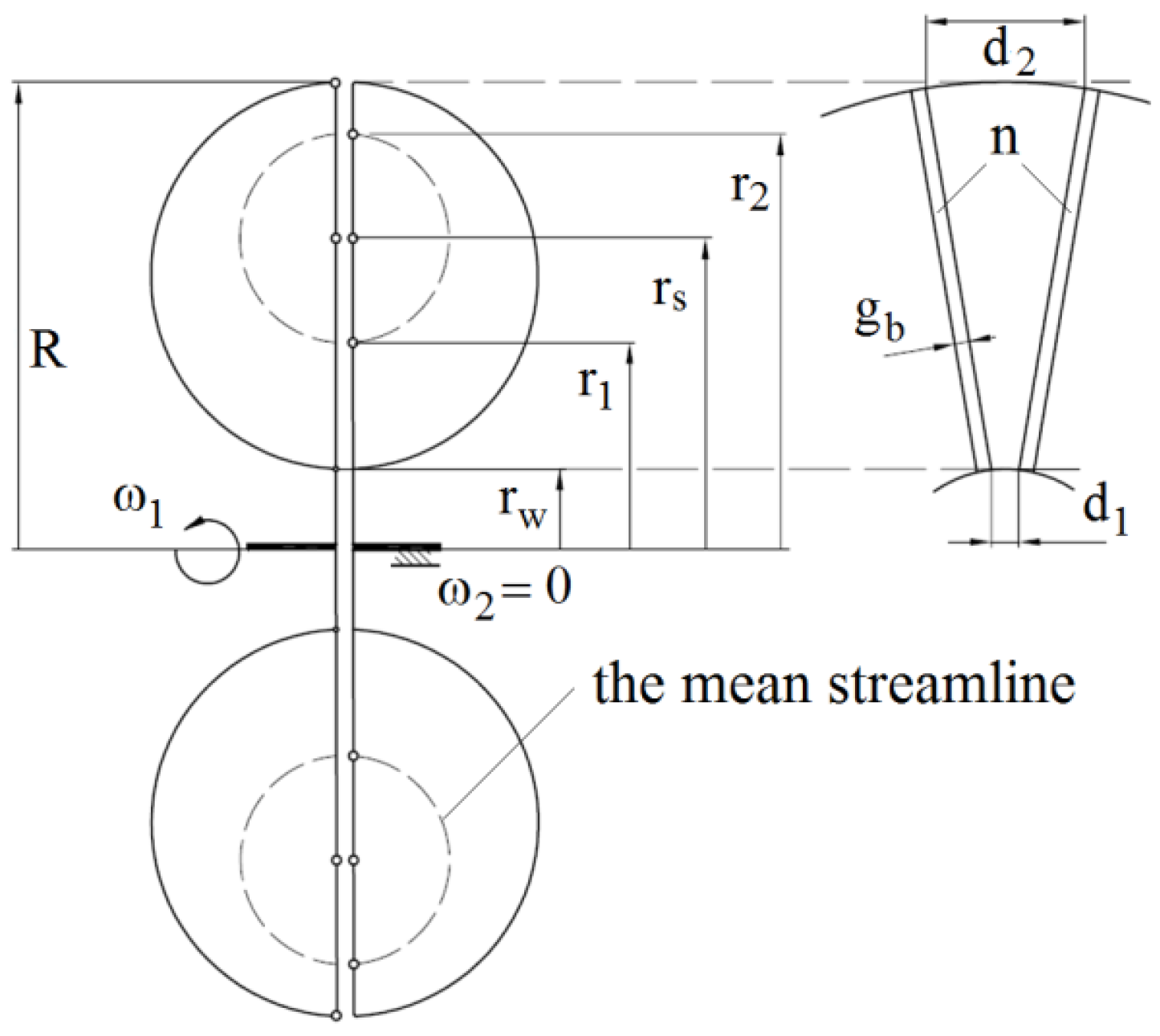
Figure 3.
PHB with the ER fluid: (a)—design solution: 1—pump, 2—turbine, 3—casing, 4—slip rings supplying the high voltage, 5—sealing; (b)—view of the pump rotor after tests: 1—blade, 2—rotor casing.
Figure 3.
PHB with the ER fluid: (a)—design solution: 1—pump, 2—turbine, 3—casing, 4—slip rings supplying the high voltage, 5—sealing; (b)—view of the pump rotor after tests: 1—blade, 2—rotor casing.
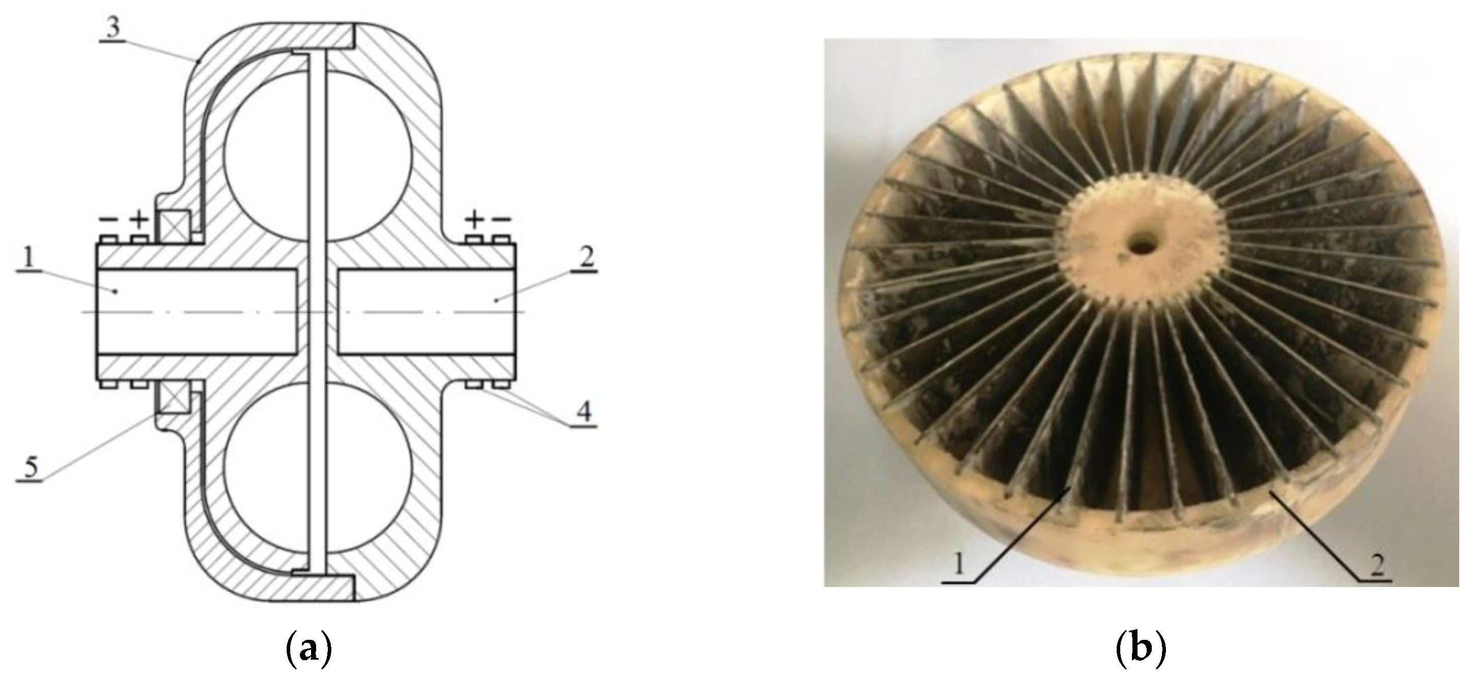
Figure 4.
Electrical circuit of the HB: re—electrical resistance of the wires, Re—electrical resistance of ER fluid, Ce—electric capacity of the HB, U1—power supply voltage, U2—voltage on the blades.
Figure 4.
Electrical circuit of the HB: re—electrical resistance of the wires, Re—electrical resistance of ER fluid, Ce—electric capacity of the HB, U1—power supply voltage, U2—voltage on the blades.
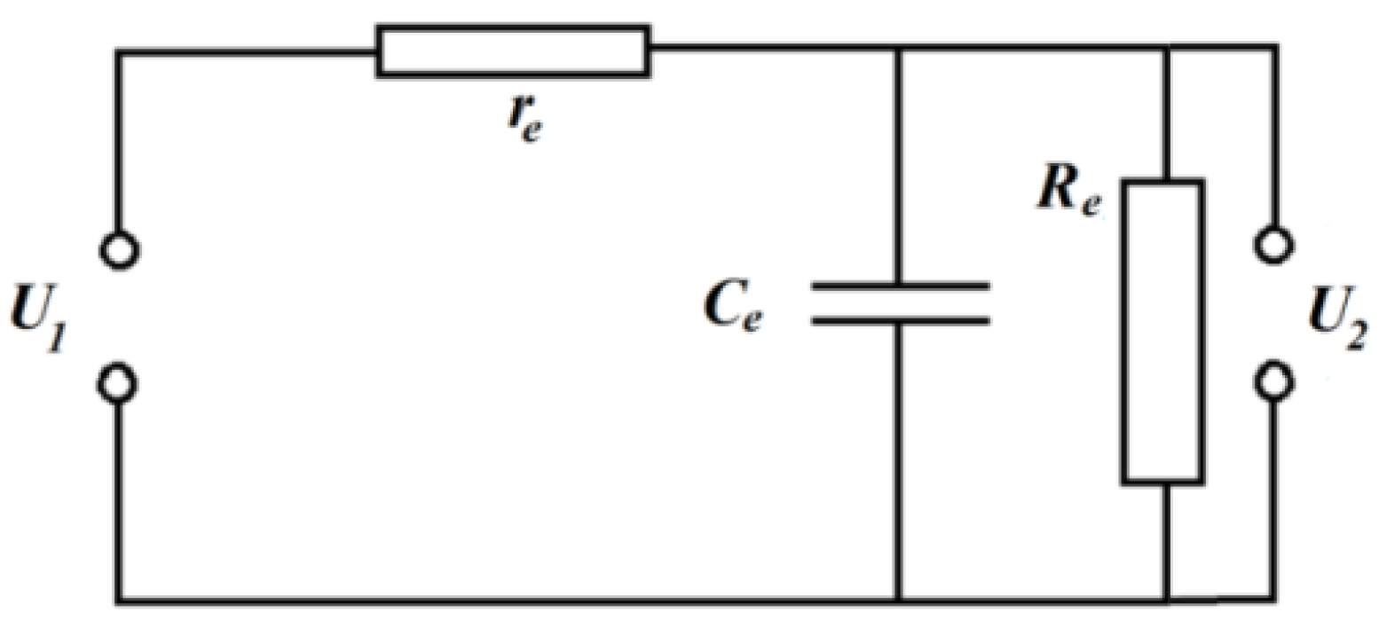
Figure 5.
Test bench scheme: 1—electric motor, 2—speed sensor, 3—slip rings used to supply high voltage, 4—the tested brake with ER fluid, 5—shaft, 6—connecting clutch, 7—torque gauge.
Figure 5.
Test bench scheme: 1—electric motor, 2—speed sensor, 3—slip rings used to supply high voltage, 4—the tested brake with ER fluid, 5—shaft, 6—connecting clutch, 7—torque gauge.
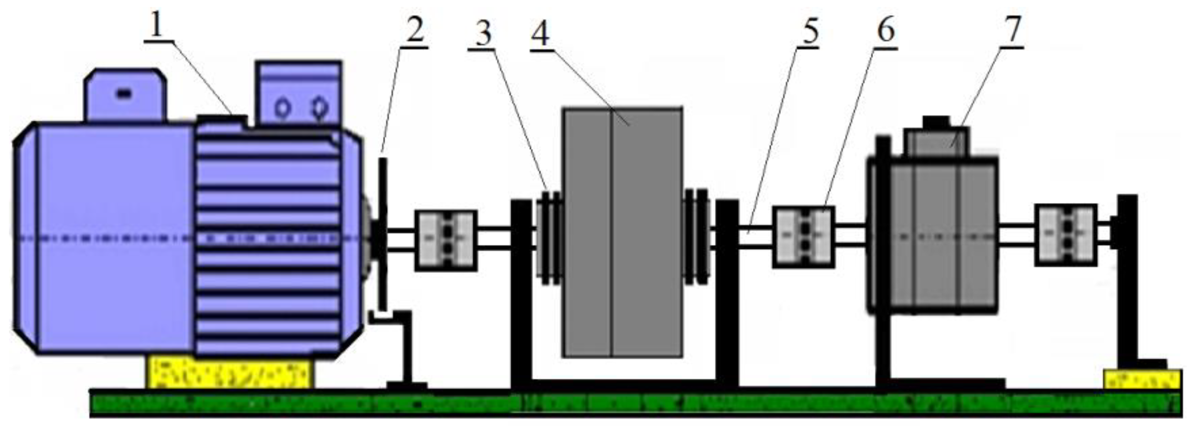
Figure 6.
Method of determining the coefficient c: solid line—model, points—test.
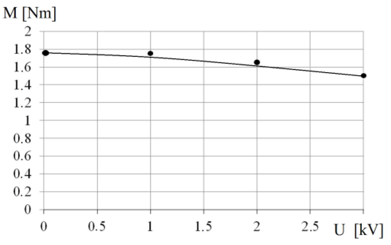
Figure 7.
Dependence of the torque on the radius rw and on the radius R.
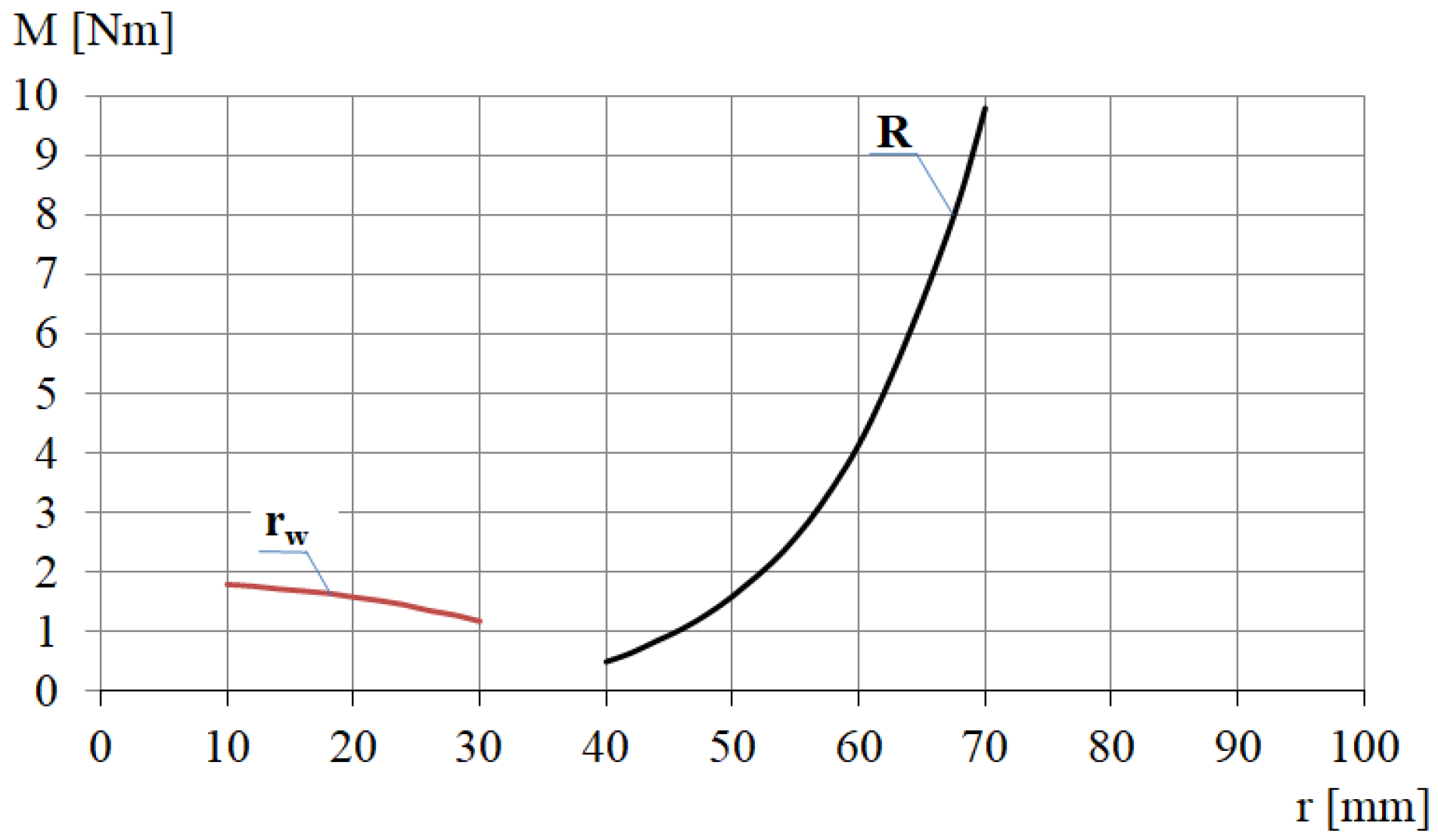
Figure 8.
Dependence of the torque M on the blade number n.
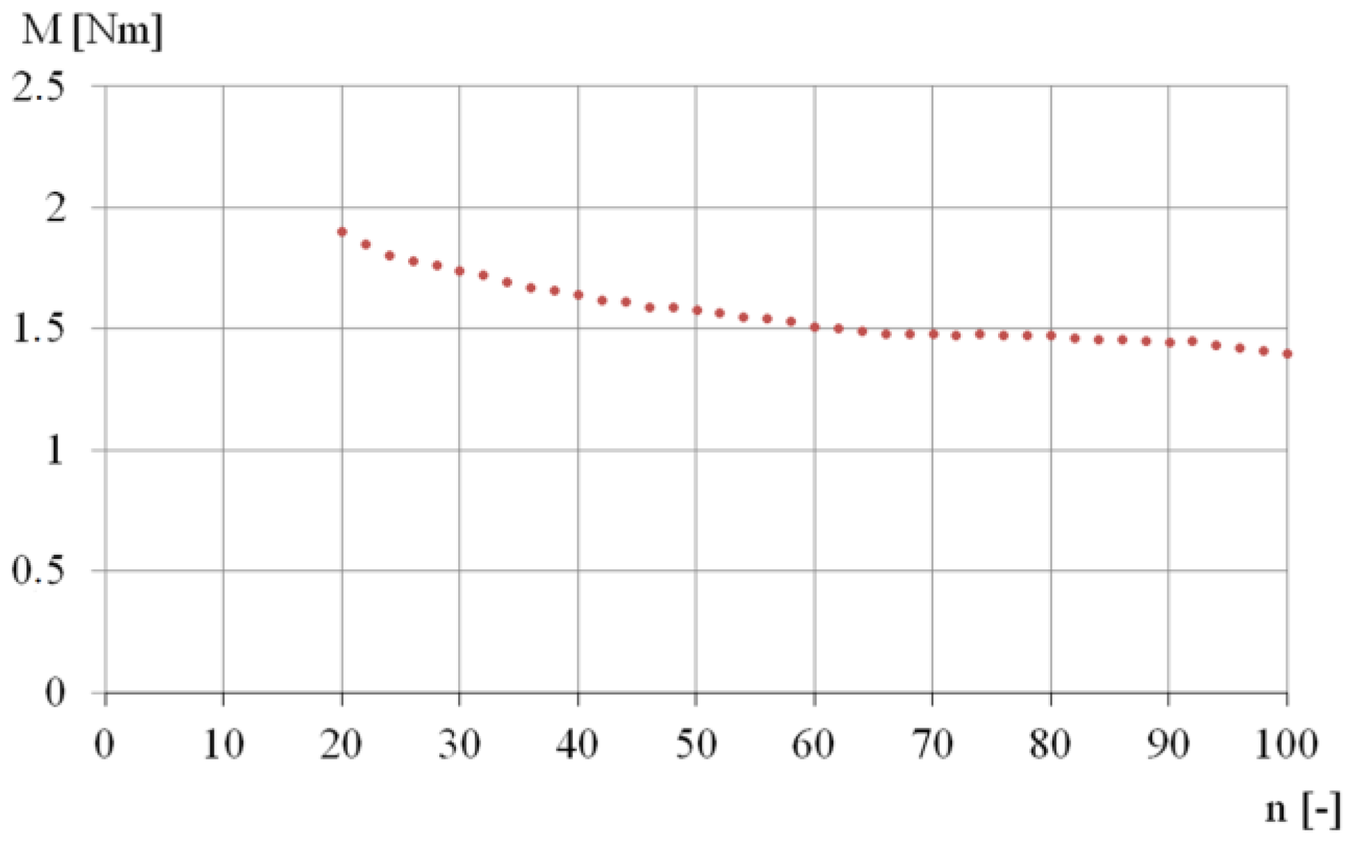
Figure 9.
Dependence of the voltage Uh on the blade number n.
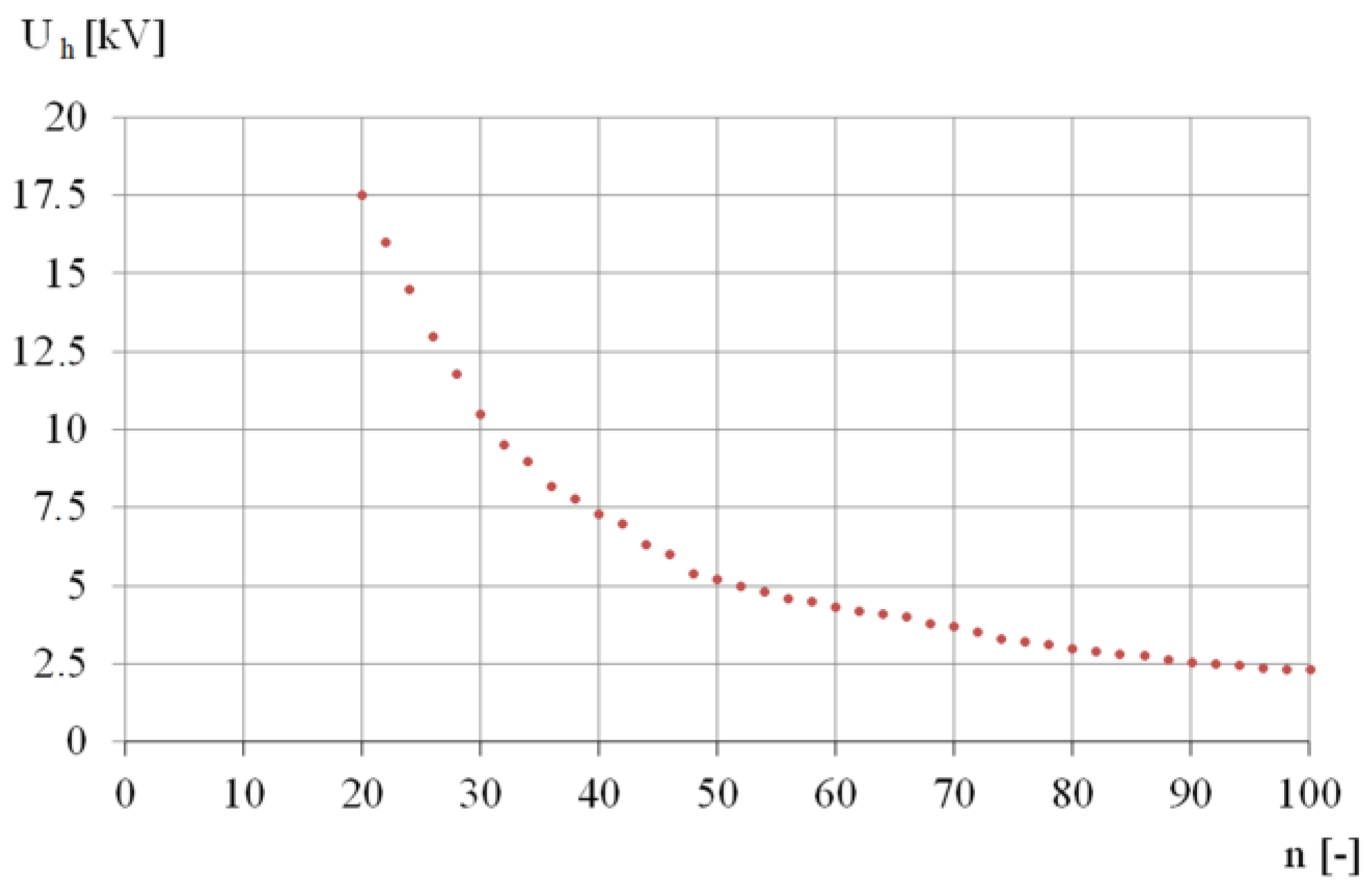
Figure 10.
Dependence of the weight G on the torque M.
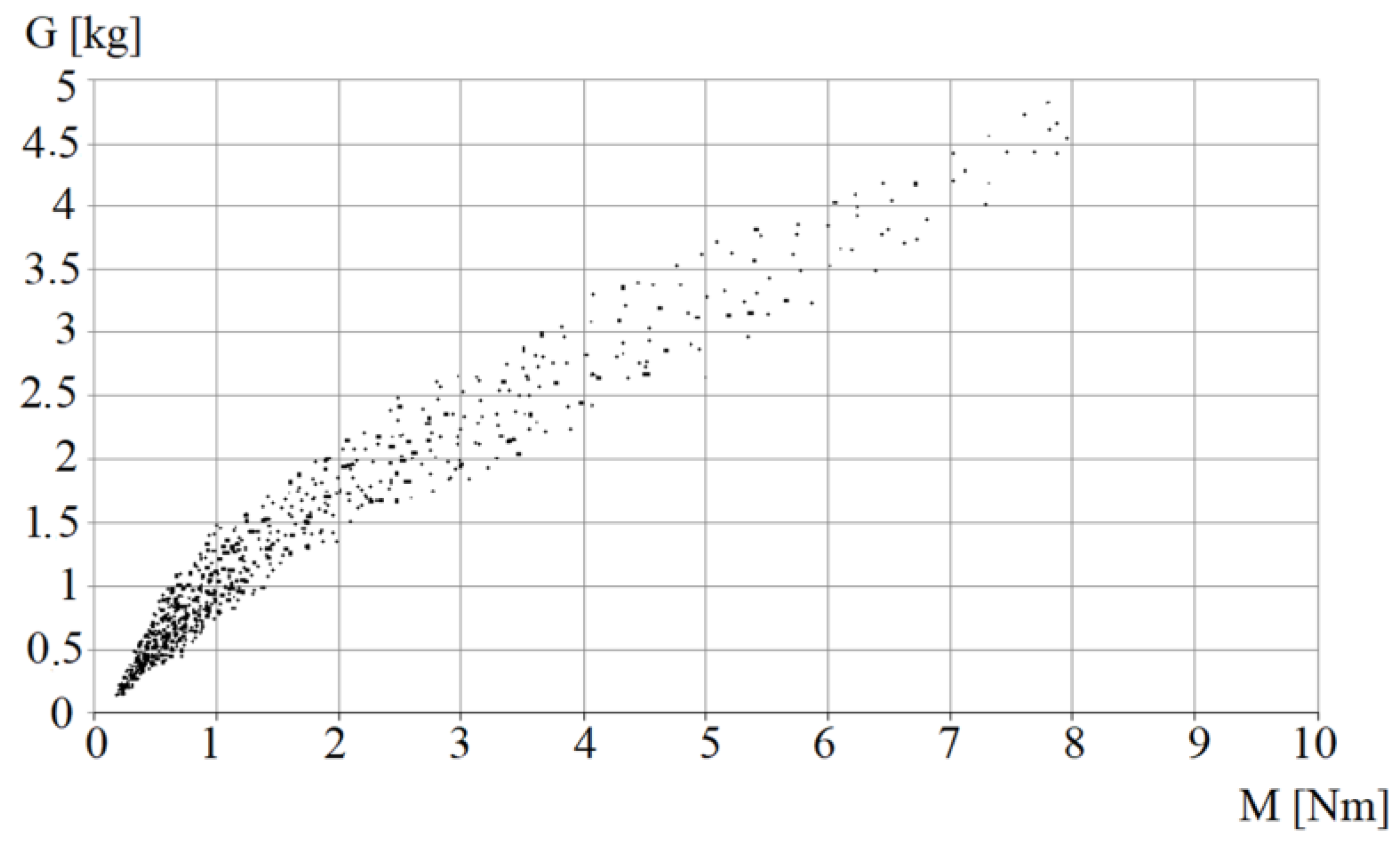
Figure 11.
Dependence of the electric power Pe on the torque M.
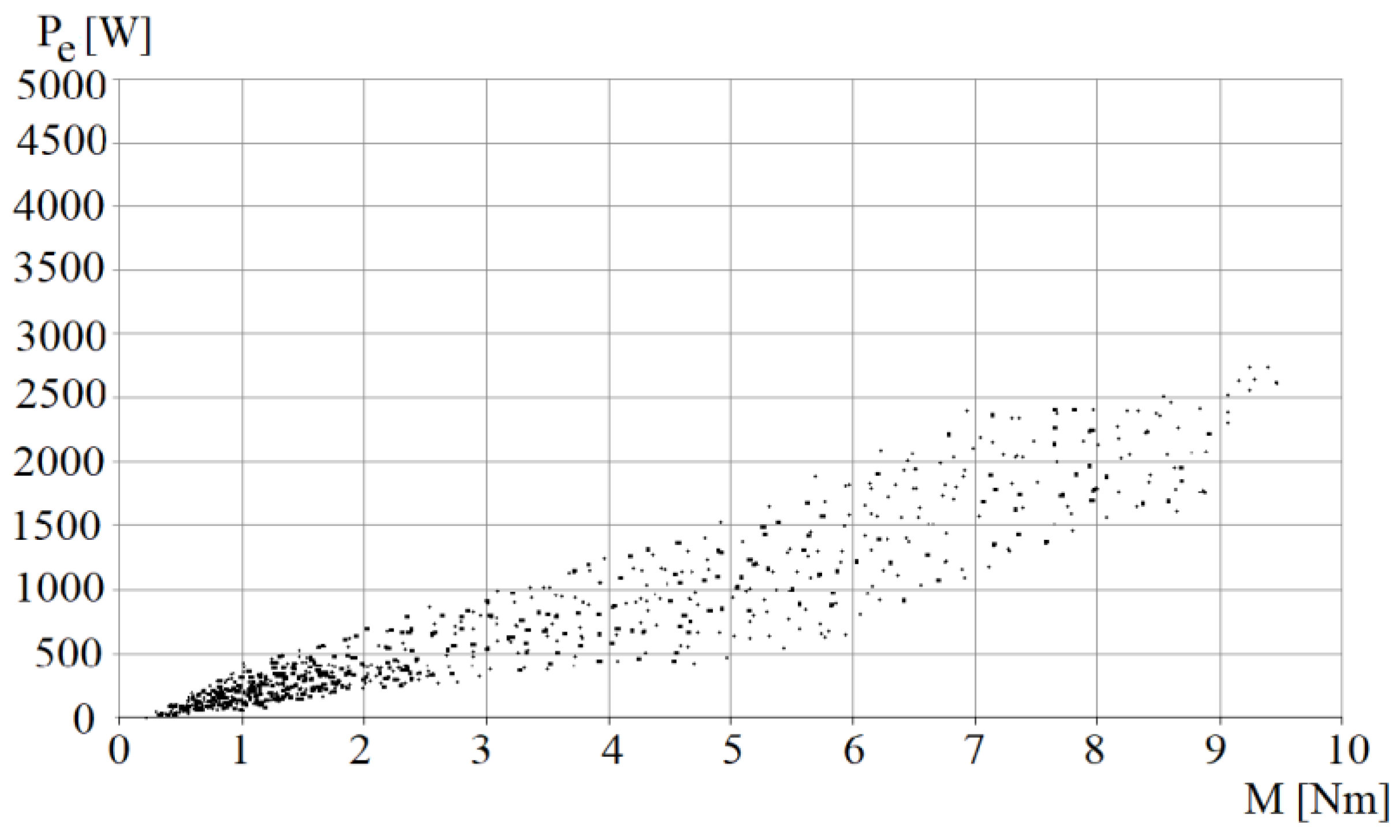
Figure 12.
Dependence of the time T on the torque M.
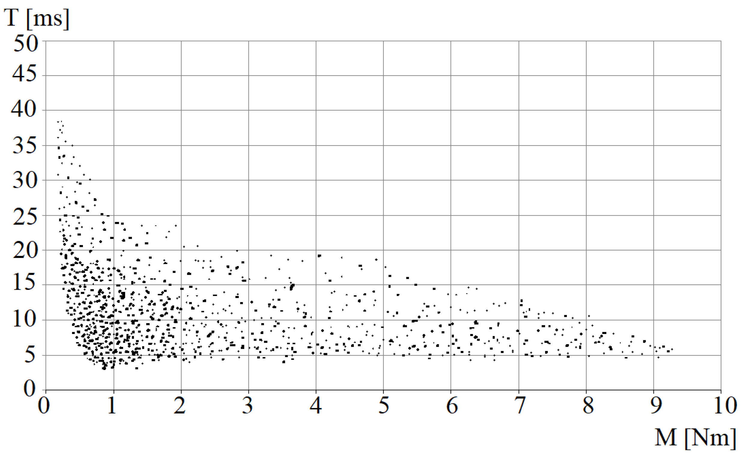
Figure 13.
Dependence of the torque M on the number of blades n.
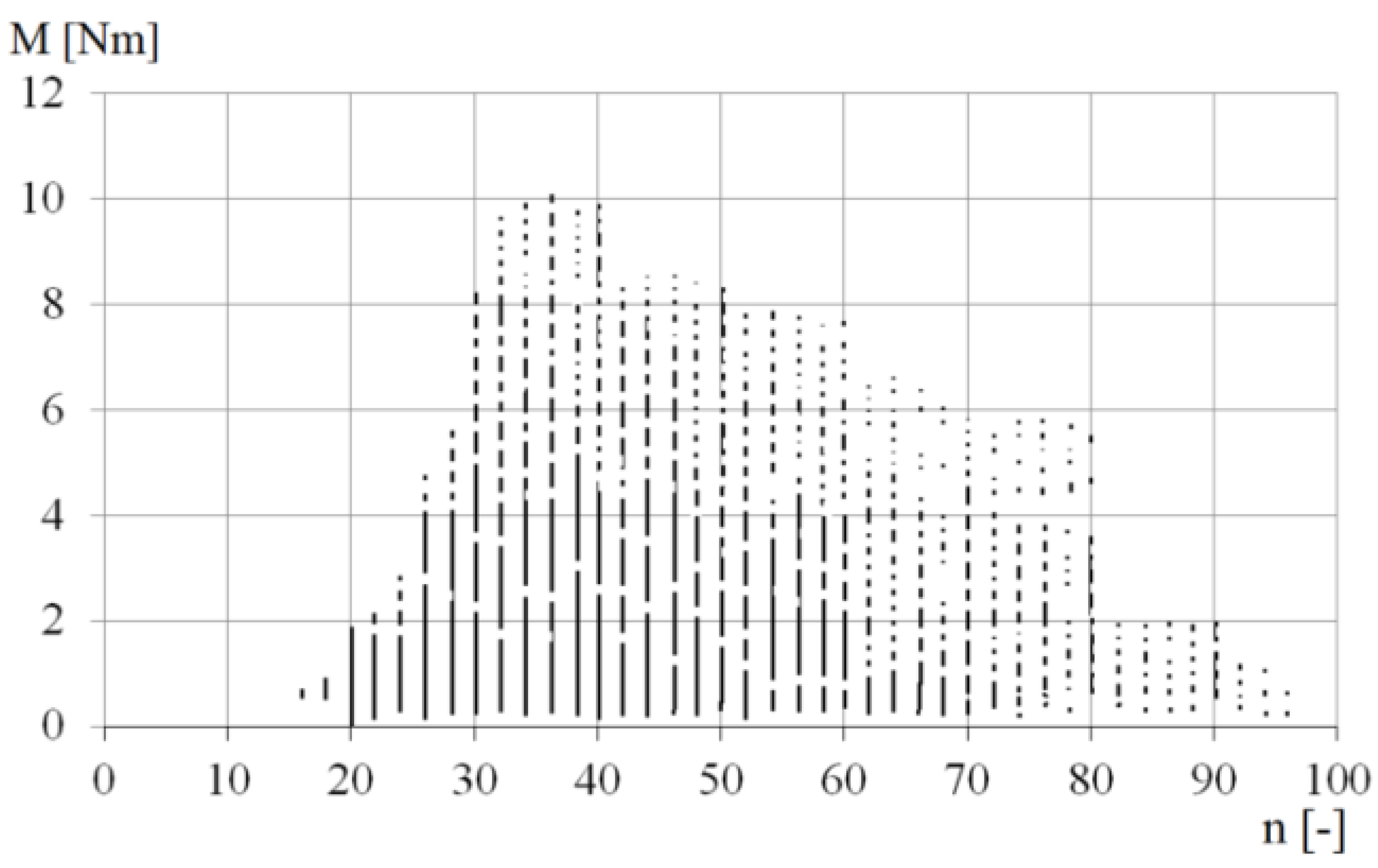
Figure 14.
Dependence of the electric power Pe on the number of blades n.
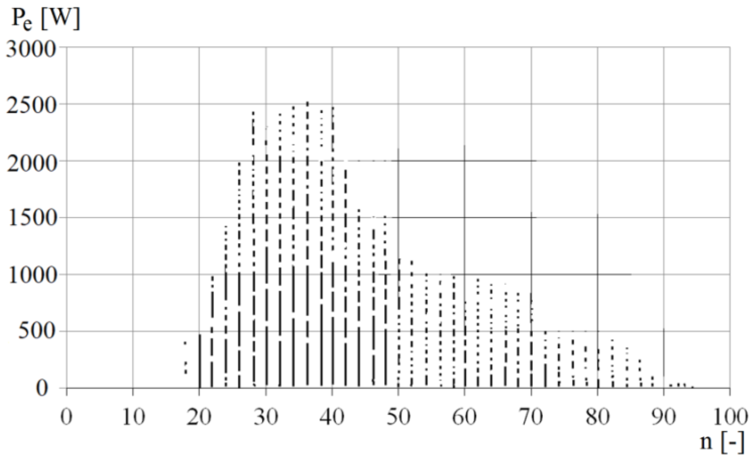
Figure 15.
Dependence of the time T on the number of blades n.

Figure 16.
Dependence of the torque M on the radius rw and on the radius R.

Figure 17.
Dependence of the electric power Pe on the radius rw and on the radius R.
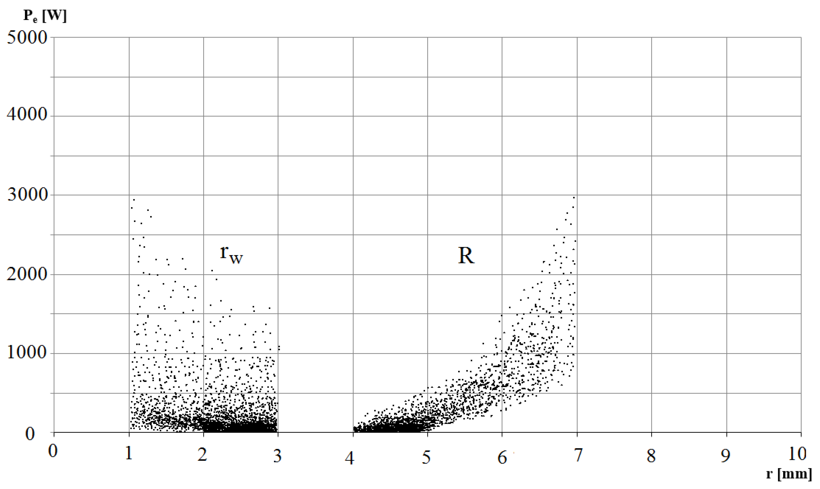
Figure 18.
Dependence of the time T on the radius rw and on the radius R.

Figure 19.
Algorithm of calculations carried out in one calculation step.
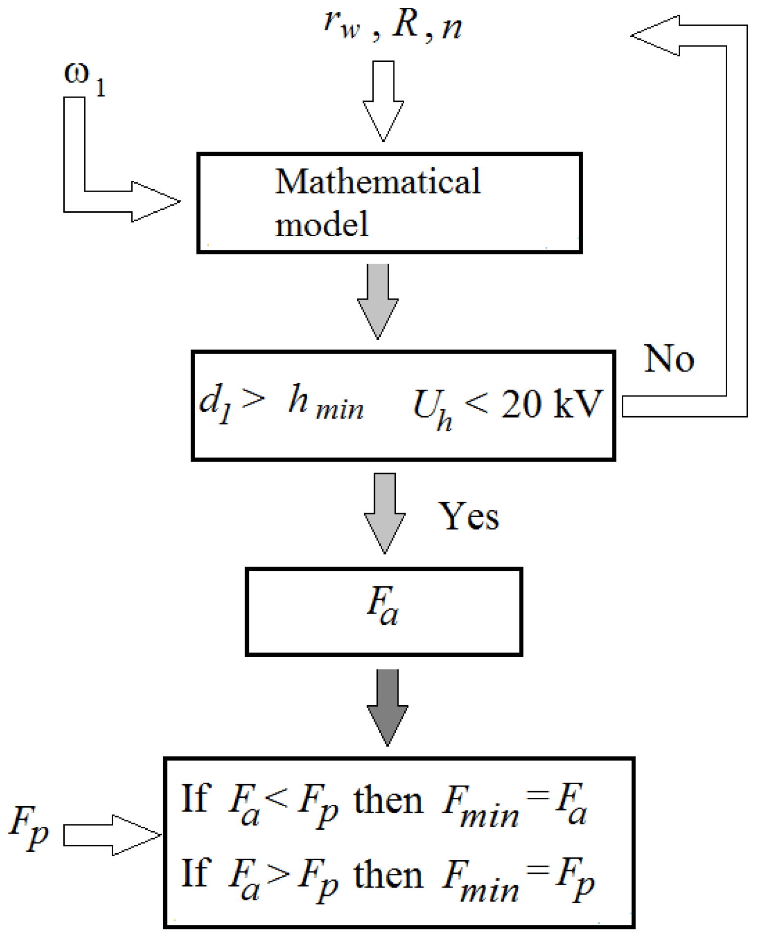
Figure 20.
Optimization results on the background of the Pareto chart: 1—FGmin, 2—FG1min, 3—FPmin, 4—FP1min, 5—FTmin, 6—FT1min, 7—PHB.
Figure 20.
Optimization results on the background of the Pareto chart: 1—FGmin, 2—FG1min, 3—FPmin, 4—FP1min, 5—FTmin, 6—FT1min, 7—PHB.


Table 1.
PHB data.
| R mm | rw mm | d1 mm | d2 mm | gb mm | n - | rs mm | r1 mm | r2 mm | ER Fluid LID 3354S |
|---|---|---|---|---|---|---|---|---|---|
| 50.5 | 15.5 | 1.5 | 7.3 | 1.0 | 38 | 37.4 | 28.6 | 44.4 |
Table 2.
Mathematical model coefficients for the researched PHB.
| Coefficient | α - | ξ - | c - | a kPa mm2/kV2 | b μA mm2/(cm2 kV2) | β - | εr - |
|---|---|---|---|---|---|---|---|
| Value Formula | 2.30 (7) | 6.64 (22) | 3.93 (23) | 0.41 (27) | 35.31 (28) | 3.00 (35) | 5.00 (37) |
Table 3.
Intervals and conditions concerning the parameters.
| Parameter Interval | Conditions | |||
|---|---|---|---|---|
| rw mm | R mm | n - | d1 mm | Uh kV |
| 10 < rw< 30 | 40 < R < 70 | 10 < n < 120 | d1 > hmin = 1 | Uh < 20 kV |
Table 4.
Requirements concerning the HB optimization criteria.
| Name | Designation | Requirements | Main Calculation Formula Numbers |
|---|---|---|---|
| Torque | M | Maximal | (16), (17), (25), (26) |
| Weight | G | Minimal | (4)–(7) |
| Electric power | Pe | Minimal | (30), (31), (33), (34) |
| Time | T | Minimal | (35)–(37) |
Table 5.
Optimization results for the whole intervals of decision variables.
| Fmin | M Nm | rw mm | R mm | n - | G/M kg/Nm | Pe/M W/Nm | T/M ms/Nm | G kg | Pe W | T ms |
|---|---|---|---|---|---|---|---|---|---|---|
| FGmin | 7.478 | 29.1 | 69.9 | 42 | 0.497 | 181.4 | 0.790 | 3.717 | 1356 | 5.9 |
| FG1min | 7.473 | 29.9 | 69.4 | 38 | 0.446 | 231.6 | 0.681 | 3.333 | 1731 | 5.1 |
| FPmin | 0.218 | 28.8 | 40.9 | 98 | 1.136 | 38.5 | 201.821 | 0.248 | 8.42 | 44.4 |
| FP1min | 0.222 | 28.9 | 41.1 | 100 | 1.150 | 38.2 | 206.113 | 0.255 | 8.45 | 45.8 |
| FTmin | 9.850 | 11.6 | 69.8 | 30 | 0.601 | 254.6 | 0.358 | 5.920 | 2508 | 3.5 |
| FT1min | 9.886 | 10.6 | 69.9 | 30 | 0.611 | 313.3 | 0.489 | 6.040 | 3096 | 4.8 |
Table 6.
Values of the ratios G/M, Pe/M, T/M and G, Pe, T for the optimized PHB.
| M Nm | rw mm | R mm | n - | G/M kg/Nm | Pe/M W/Nm | T/M ms/Nm | G kg | Pe W | T ms |
|---|---|---|---|---|---|---|---|---|---|
| 1.733 | 15.5 | 50.5 | 38 | 1.013 | 97.9 | 5.72 | 1.756 | 170 | 9.9 |
Table 7.
PHB optimization results for 1.700 Nm < M < 1.800 Nm.
| Fmin | M Nm | rw mm | R mm | n - | G/M kg/Nm | Pe/M W/Nm | T/M ms/Nm | G kg | Pe W | T ms |
|---|---|---|---|---|---|---|---|---|---|---|
| FGmin | 1.728 | 29.7 | 53.6 | 30 | 0.570 | 239.0 | 3.027 | 0.985 | 413 | 5.2 |
| FG1min | 1.782 | 28.9 | 53.6 | 30 | 0.586 | 240.9 | 3.070 | 1.044 | 429 | 5.4 |
| FPmin | 1.749 | 29.6 | 55.8 | 88 | 0.837 | 64.8 | 14.603 | 1.464 | 113 | 25.5 |
| FP1min | 1.753 | 29.6 | 55.9 | 86 | 0.823 | 66.5 | 13.986 | 1.443 | 116 | 24.5 |
| FTmin | 1.746 | 16.2 | 50.0 | 22 | 0.894 | 356.1 | 2.245 | 1.561 | 621 | 3.9 |
| FT1min | 1.795 | 12.6 | 49.8 | 22 | 0.992 | 351.0 | 2.269 | 1.781 | 630 | 4.0 |
Disclaimer/Publisher’s Note: The statements, opinions and data contained in all publications are solely those of the individual author(s) and contributor(s) and not of MDPI and/or the editor(s). MDPI and/or the editor(s) disclaim responsibility for any injury to people or property resulting from any ideas, methods, instructions or products referred to in the content. |
© 2023 by the authors. Licensee MDPI, Basel, Switzerland. This article is an open access article distributed under the terms and conditions of the Creative Commons Attribution (CC BY) license (https://creativecommons.org/licenses/by/4.0/).
Share and Cite
MDPI and ACS Style
Kęsy, Z.; Musiałek, I.; Choi, S.-B. Design Optimization of a Hydrodynamic Brake with an Electrorheological Fluid. Appl. Sci. 2023, 13, 1089. https://doi.org/10.3390/app13021089
AMA Style
Kęsy Z, Musiałek I, Choi S-B. Design Optimization of a Hydrodynamic Brake with an Electrorheological Fluid. Applied Sciences. 2023; 13(2):1089. https://doi.org/10.3390/app13021089
Chicago/Turabian StyleKęsy, Zbigniew, Ireneusz Musiałek, and Seung-Bok Choi. 2023. "Design Optimization of a Hydrodynamic Brake with an Electrorheological Fluid" Applied Sciences 13, no. 2: 1089. https://doi.org/10.3390/app13021089
Note that from the first issue of 2016, this journal uses article numbers instead of page numbers. See further details here.