

Software Operation Anomalies Diagnosis Method Based on a Multiple Time Windows Mixed Model

School of Reliability and Systems Engineering, Beihang University, Beijing 100191, China
*
Author to whom correspondence should be addressed.
Appl. Sci. 2023, 13(20), 11349; https://doi.org/10.3390/app132011349
Submission received: 16 August 2023
/
Revised: 2 October 2023
/
Accepted: 6 October 2023
/
Published: 16 October 2023
(This article belongs to the Topic Software Engineering and Applications)
Abstract
:Featured Application
This method addresses the problem of predicting anomaly data in software runtime. The proposed method utilizes multiple time windows to choose models from multiple classes of anomaly method detectors and fuses the anomaly results in order to save the process of anomaly detection model selection. In practice, the technique can make timely predictions and alerts for anomalous operation.
Abstract
The detection of anomalies in software systems has become increasingly crucial in recent years due to their impact on overall software quality. However, existing integrated anomaly detectors usually combine the results of multiple detectors in a clustering manner and do not consider the changes in data anomalies in the time dimension. This paper investigates the limitations of existing anomaly detection methods and proposes an improved integrated anomaly detection approach based on time windows and a voting mechanism. By utilizing multiple time windows, the proposed method overcomes the challenges of cumulative anomalies and achieves enhanced performance in capturing anomalies that accumulate gradually over time. Additionally, two hybrid models are introduced, based on accuracy and sensitivity, respectively, to optimize performance metrics such as AUC, precision, recall, and F1-score. The proposed method demonstrates remarkable performance, achieving either the highest or only a marginal 3% lower performance compared to the optimal model.
1. Introduction
In recent years, the importance of detecting anomalies in software systems has become increasingly evident. As software has become more prevalent in our daily lives, ensuring its quality has become crucial. Software failures have been linked to catastrophic accidents, highlighting the need for effective anomaly detection [1]. Moreover, the economic impact of software bugs and failures is substantial, with an estimated annual cost of $59.5 billion to the U.S. economy alone [2]. However, the task of identifying and diagnosing software faults poses significant challenges.
One limitation of anomaly detection in software is the inability to pinpoint the exact location of a true fault using real-time operational data. Traditionally, fault identification relies on the fault time and human expertise, rather than real-time data analysis. This approach is not efficient for modern software systems that generate vast amounts of operational data. To address this issue, the emergence of unsupervised learning techniques has provided a methodological foundation for detecting anomalies in real-world software.
Numerous unsupervised anomaly detection methods have been developed, including those available in the PYOD (version 1.1.0) [3] module for Python. These methods encompass linear models based on proximity, statistical approaches, abnormality combinations, and neural networks. However, determining the most suitable unsupervised anomaly detection method for a specific software failure time series dataset is not straightforward. The selection of optimal anomaly detectors requires research and exploration of integrated outlier detection methods.
An integrated detector combines the results and performance of multiple types of detectors, increasing the chances of achieving better detection outcomes. However, the effectiveness of the integrated detector heavily depends on the chosen integration method. If the integration is poorly executed or the results are not adequately combined, the predictive ability of the integrated detector will suffer.
Existing anomaly detection integrators encompass several approaches dominated by voting-based, weighted average-based, stacking-based, and data clustering-based methods. However, in the realm of software operation anomalies, most anomalies do not simply manifest abruptly. For instance, studies focused on collecting performance data, such as CPU and memory usage, have revealed a discernible tendency for these metrics to transition from normal to abnormal states. In the context of predicting software anomalies, certain methods aim to forecast performance anomalies in advance. These approaches leverage techniques such as long and short-term memory neural networks to capture the typical behavior of a system and identify early deviations that may serve as precursors to an impending anomaly. This observation further underscores the temporal and predictable nature of software anomalies [4,5]. Nonetheless, existing integrated detectors primarily emphasize the distribution and clustering of anomaly data. This emphasis poses challenges when attempting to incorporate the gradual accumulation of anomalies over time into the anomaly detection process. Although the clustering method is good at separating anomalous data from normal data, it is not effective for cumulative anomalies [6].
Therefore, this study considers an integrated anomaly detection method based on time windows. Considering that the cumulative time of anomalies is difficult to grasp and fix, this paper investigates the use of multiple time windows in combination with a voting mechanism to circumvent the anomaly advancement or lagging problem brought about by a single time window. Meanwhile, this paper proposes two hybrid models that combine the detection results of multiple anomaly detection basics, which can simultaneously deal with sudden and cumulative anomalies.
The main contributions of this paper are as follows:
- Proposing an improved integrated anomaly detector that utilizes multiple time windows and a voting mechanism to enhance the detection of cumulative anomalies. By incorporating information from different time windows, the detector achieves enhanced performance in capturing anomalies that accumulate gradually over time.
- Introducing two anomaly-integrated models based on accuracy and sensitivity, respectively. These models provide effective integration of anomaly detection results, aiming to optimize performance metrics such as AUC, precision, recall, and F1-score. The proposed models demonstrate remarkable performance, achieving either the highest or only a marginal 3% lower performance compared to the optimal model.
These contributions address the need for an advanced integrated anomaly detection approach that considers the cumulative nature of anomalies and optimizes performance metrics. The proposed techniques have the potential to significantly improve anomaly detection accuracy and effectiveness in various domains.
2. Related Research
2.1. Software Fault Detection Method
Software reliability prediction and evaluation technology remains a popular research topic and also implies the prediction of the possibility of software failure. Researchers [1,2] have investigated the future directions of architecture and fault data. Reliability diagnosis based on architecture uses the Markov model and various extended models, and also uses the failure rate information and path of the modules in the software. State transition predicts the reliability of the software system. Reliability diagnosis based on fault data uses the fault interval data and cumulative fault data collected in the reliability test to propose statistical models to evaluate the operating status of the system.
Current software fault diagnosis methods primarily include statistical methods and machine learning methods. Based on this development, a model that combines these two methods is used to diagnose software faults [7]. Software failure prediction models based on statistical methods primarily include many regression models, such as logistic regression, negative binomial regression, Poisson regression, and multiple zero negative binomial regression models. Since the relationship between software failure and data rarely has a direct linear correlation model, the most basic linear regression is not applicable to software failure prediction. Logistic regression improves upon linear regression because linear regression has difficulty classifying results when there is an illegal probability value other than 0–1; thus, logistic regression uses logarithmic transformation, and the result can be any value in the range of negative infinity to positive infinity. Taghi et al. [8,9] proposed a generalized classification rule to solve the problem that the logistic regression model could not perform a quantitative quality prediction. They conducted case studies on two industrial software systems and developed each system. Two counting models (PRM and ZIP) and one classification model (LRM) were used. Andrea Janes et al. [10] used statistical models that were suitable for nonnormally distributed count data, such as Poisson regression, negative binomial regression, and multiple zero negative binomial regression models, using correlation, dispersion coefficient, and the Alberg diagram on the same dataset as the evaluation criterion.
Machine learning algorithms have long been widely used for software fault diagnosis. The primary machine learning algorithms used are naive Bayes, Bayesian networks, support vector machines (SVMs), random forests, artificial neural networks, and other methods. Tim Menzies et al. [11] compared the classification performance of naive Bayes and decision trees. After logarithmic processing of the data, the training method of naive Bayes can achieve better classification results. Shiqing Jia et al. [12] used a multisource linear regression algorithm to analyze and diagnose web server parameters in detail based on the software aging phenomenon. Domenico Cotroneo et al. [13] performed defect data analysis on three large software projects to collect data on age-related errors (ARBs). Naive Bayes, Bayesian networks, decision trees, and other methods were used to construct a fault diagnosis model. Ref. [14] proposed a timed error detection framework that combines systematic interleaving of recorded instructions in source code with two detection algorithms to achieve error detection for two real-world critical information systems.
2.2. Development of Anomaly Detectors
The earliest anomaly detectors were derived from linear models. LMDD, OCSVM, and PCA are representative of linear models. This type of model primarily focuses on the deviation or dissimilarity of the data and uses a linear model to find possible interference values from a series of similar data. These interference values may be anomalous objects to look for [15,16,17].
Proximity-based detection is also a major research topic of anomaly detectors. KNN (k nearest neighbors) was developed first and judges abnormal data using the distance to the k-th nearest neighbor as an outlier. Many variants have also been developed based on KNN, such as AvgKNN and MedKNN [18,19]. In addition to KNN, other neighboring anomaly detectors can be identified according to different specified outlier sources. Methods such as LOF, COL, and CBLOF use different outlier factors to discriminate and process abnormal data [20,21,22]. HBOS uses histograms to obtain abnormal points in the series of data [23]. The closest proximity detector is ROD (rotation-based outlier detection) [24], which learns local spatial attributes and uses Rodrigues’ rotation formula to construct anomaly scores. This method does not require distribution assumptions and achieves good performance during forecasting.
The development of neural networks has also created new research directions for anomaly detection. More mature neural network detectors include AutoEncoder and VAE [25]. A self-encoding neural network is an unsupervised learning algorithm that uses a back propagation algorithm and makes the target value equal to the input value, making this type of algorithm more suitable for high-dimensional complex data. The cutting-edge neural network detectors also include SO_GAAL and MO_GAAL [26]. By generating confrontation, the generator creates abnormal data from random noise, and the discriminator determines whether the data generated are abnormal or original and normal. In the final abnormality detection process, it is only necessary to use the discriminator to determine whether data are normal or abnormal.
2.3. Anomaly Detection Integrator
An integrated anomaly detector is a sophisticated approach that combines multiple anomaly detection techniques or models to improve the accuracy and effectiveness of anomaly detection in various domains, including software systems, industrial processes, cybersecurity, and more. Instead of relying on a single detector, an integrated anomaly detector leverages the collective strength and diversity of multiple detectors to enhance the overall detection performance [27].
The integration process involves combining the outputs or predictions of individual anomaly detectors to generate a consolidated result. This integration can be achieved through different methods, such as voting, weighted averaging, stacking, or clustering [27,28,29]. The choice of integration method depends on factors like the nature of the data, the characteristics of the anomaly detection models, and the specific objectives of the detection task.
The integrated anomaly detector offers several advantages over using a single detector. By combining multiple detectors it can leverage their complementary strengths and mitigate their individual weaknesses. This leads to improved detection accuracy, robustness, and the ability to handle a wider range of anomaly types and patterns. Moreover, the integrated detector can provide more reliable and confident anomaly alerts or predictions, as it takes into account multiple perspectives and evidence [29].
Two recent outstanding representative anomaly detectors are LSCP [30] and SUOD [31]. LSCP uses the consistency of the nearest neighbors in randomly selected feature subspaces to define the local area around the test instance, thereby selecting the best detector and optimizing the detection result to a certain extent. SUOD focuses on solving the efficiency problems caused by using multiple detectors. SUOD designed three acceleration modules to optimize the anomaly detection process from three levels of data, model, and execution and achieved better experimental results.
However, existing studies rarely incorporate the cumulative properties of anomaly data over time-varying anomalies into anomaly detection [4,5,6]. Both weighting-based and clustering-based identify anomalies from the characteristics of the data itself. For sudden anomalies, these methods play a good supervisory role. But for cumulative anomalies, these methods have some limitations.
3. Anomaly Detection Synthesis Algorithm Based on Multiple Time Windows
Different algorithms examine the abnormal state of high-dimensional data from their own perspectives, but none can completely describe the anomaly. To fully identify possible data anomalies, an ensemble learning framework was designed to comprehensively use various newer algorithms. The algorithms used are from the 11 algorithms in the PYOD [3] library of the Python language, as shown in Table 1.
To improve the adaptability between the algorithm and the data, a comprehensive anomaly detection algorithm based on multiple time windows is proposed in this section. This algorithm uses a time window to search for a sequence of anomaly detection algorithms that is suitable for the training set. Two criteria of accuracy or sensitivity were used to fuse the anomaly detection algorithm, and the comprehensive anomaly score and anomaly label were calculated. The overall detection scheme is shown in Figure 1.
3.1. Automatic Selection of Detectors Based on Multiple Time Windows
This section describes how to select the most similar and optimal multiple detectors from multiple anomaly detection models.
As shown in Figure 2, the steps of this method are as follows:
- Training data are input into 10 anomaly detection algorithms for training, and each algorithm obtains a set of anomaly scores.
- Multiple time windows are selected, where each time window refers to a continuous set of data.
- The time windows are cycled through, as shown in Figure 3.
- 3.1
- We set the sample data corresponding to the largest n scores with the same number of windows in each group as an abnormal label.
- 3.2
- We randomly generate adjacent spaces. The default number of random times is 1/3 to 1/2 of the total sample data. The length of the adjacent data is equal to the length of the time window. We then find the space with the largest number of abnormal tags in this space and the front and rear spaces.
- 3.3
- We record the model sequence with abnormal labels in the adjacent space obtained in the previous step.
- 3.4
- We repeat steps 3.1 to 3.3 for the models that did not appear in 3.3 to obtain the second set of model sequences.
- The anomaly scores and anomaly labels of the two sets of the model sequences obtained in step 3 are then fused as the final detection result.
The first step is to put the training data into each anomaly detection algorithm for training and to obtain each anomaly score and anomaly label.
For each set of abnormal tags, multiple sets of model selection tags are generated with different time windows. The label setting condition is the position corresponding to the largest scores, where n is equal to the length of the time window. We select labels for multiple sets of models in the same time window and generate a neighboring space to count the number of abnormal labels in the space. For data group with different total numbers of abnormal labels, the number of spatial abnormal labels should be multiplied by the corresponding weight , which is determined by the real number of abnormal labels and the set number of labels . The calculation method is shown in Formula (1). In this study, we assume that if there are anomalies in the dataset, there should be multiple anomaly detectors that can identify most of the typical anomalies. The goal of this step is to use a random neighboring space to find these abnormal points recognized by multiple detectors.
Then, we count the number of detectors with abnormal tags in the abnormal space centered on this abnormal point. As shown in Figure 4, taking the median of the total as the dividing line, we select the detector that is larger than the dividing line. These detectors are the results found by this time window. We then count the detector results multiplied by the coefficient of and select the detector with more than half of the occurrences as the final result.
Concurrently, we identified another situation. The best multiple detectors did not appear in the anomaly space during the first iteration; this likely occurred because the number of different types of anomaly detectors selected were not exactly the same, resulting in the best detectors not necessarily appearing in the space with the most anomalies. Therefore, the secondary selection strategy was used in this study, as described in step 3.4. The detectors that did not appear in the first round are optimized again based on the time window. In subsequent steps, the performance indicators of the two rounds of results are calculated concurrently, and the best are selected for use.
3.2. Model Integrated Based on Accuracy or Sensitivity
Section A filters out suitable multiple anomaly algorithm detectors with better results for the dataset. This section introduces how to integrate the results of these anomaly detection algorithms to make the final anomaly result reach the optimal or suboptimal result.
For each detector, its results on the test set contain two results: anomaly score and anomaly label. First, for each group of abnormal scores, to facilitate their integration, the respective scores are standardized by Z score. The conversion formula is shown in Formula (2). The purpose is to scale the scores that are inconsistent in each interval so that they fall into a specific interval for integration:
where is the sample mean and is the sample variance.
Next, for the fusion of anomaly scores and anomaly labels, there are two solutions in this study, one based on accuracy and one based on sensitivity. The formula based on accuracy is as follows (3) and (4):
where A is the anomaly score; L is the anomaly label; i refers to the i-th sample; D is all the selected anomaly detectors; and num(D) counts the number of anomaly detectors.
When accuracy is most important, the abnormal label in this study is set to one when half or more of the selected algorithms report that there is an abnormality in the sample data. The final score is the average of the standardized scores of all models considered abnormal. This fusion calculation considers as much information as possible to reduce the false alarm rate in real fault diagnosis and to improve the accuracy of fault diagnosis.
The formula based on sensitivity is as follows:
where A is the anomaly score; L is the anomaly label; i refers to the i-th sample; D represents all the selected anomaly detectors; and num(D) counts the number of anomaly detectors.
When sensitivity is most important, the label of the point is set equal to one if the abnormal label of a certain point of sample data is identified as one using a specific model. This method tries to eliminate as many abnormalities as possible. All points are considered. In most cases, this method will reduce the recall rate of the model. However, in a real application, the two modes have their own advantages and disadvantages, as shown and analyzed in the experiments described below.
4. Experiments Design
In this study, we have designed four sets of validation experiments. The first set of experiments focuses on examining the impact of different time windows on the detector’s ability to identify anomalies. It presents the results under various combinations of time windows. The second set of experiments builds upon the findings from the first set and compares the integration results with those of the basic anomaly detector. The objective is to validate the effectiveness of the anomaly integration algorithm presented in Section 3. In the third set of experiments, we compare the proposed method with existing integration methods. These experiments evaluate the results against the original 10 basic anomaly detectors using publicly available real datasets. Lastly, the fourth set of experiments explores the application of this comprehensive set of methods on real software. Its aim is to demonstrate the feasibility and effectiveness of the proposed software fault diagnosis methods.
4.1. Dataset
In this section, seven real-time series derived from the real world were used as experimental objects. Their characteristics are shown in Table 2 and Table 3 [32,33].
SKAB data comes from the dataset skoltech anomaly benchmark (SKAB) [32], which contains 34 datasets with collective anomalies. Ad-cpc, Occu, speed, and twitter come from NAB [33], which is a novel benchmark for evaluating algorithms for anomaly detection in streaming real-time applications. This dataset consists of over 50 labeled real-world and artificial time series data files and includes a novel scoring mechanism designed for real-time applications. These datasets contain only one-dimension, and few abnormal points exist. Vowels and cardio come from the ODDS and DAMI. Since the algorithm proposed in this study uses a continuous time window, simple random proportional sampling cannot be used to divide the training and validation sets. Therefore, for each dataset, two sets of continuous data are selected as the test and verification sets.
For the experimental results, we have used AUC, precision, recall, and F1 as evaluation criteria. These metrics are widely used in outlier research and can be used to analyze the results.
4.2. Anomaly Detector Selection
For the base anomaly detector, we have selected the 10 anomaly detection methods listed in Table 1. In this study, the proposed methods are denoted as mixModel-pre and mixModel-sen, representing the precision-based integration model and the sensitivity-based integration model, respectively. To compare these integration models, we have chosen LSCP [30], which is a method that prioritizes integrated anomalizers following the clustering of anomaly data.
To enhance the understanding of the integration models’ capabilities, the study introduces two distinct models: mixModel-pre and mixModel-sen. These models focus on precision and sensitivity, respectively, which are essential aspects of anomaly detection. By separately considering these two dimensions, the study aims to provide a comprehensive evaluation of the integration models’ performance in capturing anomalies effectively.
To benchmark the performance of the integration models, LSCP is employed as a reference. This method utilizes clustering techniques to enable effective integration of multiple anomaly detectors, ultimately enhancing the overall detection capabilities.
Our expectation for the method presented in this study is that it has the potential to optimize one or more of the numerous anomaly detectors that exhibit similar anomaly detection outcomes. By integrating the results of these detectors, we anticipate achieving anomaly detection results that are consistent with the optimal model or demonstrate only a marginal decrease in performance.
Furthermore, it is important to highlight that, prior to the experiments, we optimized the hyperparameters of the 10 base detectors using Bayesian optimization. However, it should be noted that this optimization was conducted within a specific range and may not be generalizable to all datasets. The primary objective of this paper is to explore the selection of suitable detectors for integration based on the time window, rather than delving into the hyperparameter optimization problems of the individual models. Hence, to ensure consistency and prevent the influence of varying hyperparameter combinations on the experimental results, we directly employed the same hyperparameter settings for all detectors. The specific parameter configurations for each detector can be found in Table 4.
4.3. Experimental Design
4.3.1. Impact of Different Time Windows on Model Selection
This experiment was designed to demonstrate the intermediate process of the model preference method and its effectiveness, and discusses the implications of combining different time window intervals. The datasets used in this experiment are the seven datasets introduced in Section 4.1. Each of these different time windows is retrained data and recognized.
4.3.2. Comparison of Anomaly Detection Algorithms
This experiment compares the performance of the proposed anomaly detection integrated algorithm based on a time window and 10 basic anomaly detection algorithms. Firstly, 10 basic detectors are used to train and detect each dataset to obtain anomaly scores. After obtaining the integrated algorithms through the model optimization algorithm introduced in Section 3, their results are fused from the perspective of accuracy and sensitivity and compared with the results of the basic detector. The datasets used in this experiment are the seven datasets introduced in Section 4.1. The data in this experiment are the average values obtained from five replicates.
4.3.3. Comparison of Integrated Methods
In order to verify the effectiveness of the two integrated methods proposed in Section 3, we designed a set of experiments for validating their effects. In this study, we use the previously mentioned LSCP anomaly detection integration method as an experimental baseline. The datasets used in this experiment are the seven datasets introduced in Section 4.1. The data in this experiment are the average values obtained from five replicates.
4.3.4. Instance Validation
This experiment is designed to validate the effectiveness of the methods on a real software anomaly dataset. We considered tomcat (version 8.0.37) as an experimental object, and the selected fault was to use the stress testing tool Jmeter (version 5.6.2) to make tomcat run until the Java produced memory overflows, which causes tomcat to crash. Tomcat is a core project of the Apache Software Foundation’s Jakarta project. Tomcat is popular among Java enthusiasts and is recognized by some software developers. It is a popular web application server. The characteristics of the running data collected during the tomcat running process are shown in Table 5.
5. Result and Discussion
This section will present each of the four experimental results presented in Section 4 and their discussion.
5.1. Impact of Different Time Windows on Model Selection
In this experiment, we present the results obtained by applying different time windows to the preferred method proposed in Section 3.1. The analysis focuses on the SKAB, occu, and cardio datasets. We computed the anomaly data distribution plots for each dataset using time windows set to 2, 10, 20, 30, 40, 50, and 60, respectively. These datasets were carefully chosen as they originate from diverse data sources and exhibit distinct anomaly characteristics.
The selected datasets encompass various anomaly types, including cumulative anomalies, transient anomalies, and cases with multiple anomalies. These characteristics are visually represented in the graphs, enabling a comprehensive comparison that showcases the effectiveness of our method in handling different dataset characteristics.
For a more detailed explanation, we have included the experimental data and analysis of the remaining datasets in Appendix A. This additional information provides additional insights into our methodology and its performance across various datasets.
In these plots, the vertical axis represents the anomaly labels. The anomaly labels were determined based on the anomaly scores, which range from 0 to 1, within a fixed number (i.e., the time window). For instance, when the time window is set to two, the two highest anomaly scores are considered anomalies (labeled as 1), while the remaining scores are considered non-anomalies (labeled as 0). It is possible to observe labels in the graph that exceed the specified number. This occurs when multiple anomaly scores have the same value, leading to additional instances labeled as anomalies.
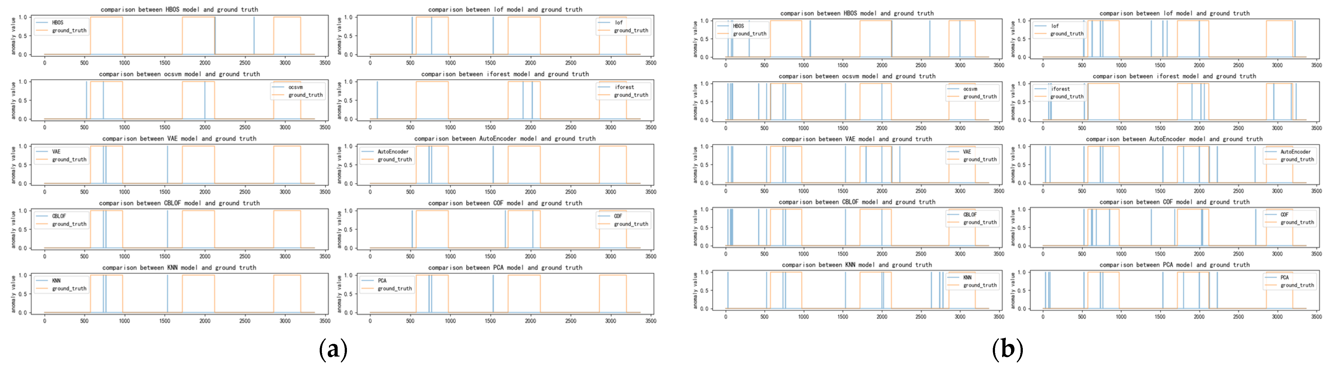
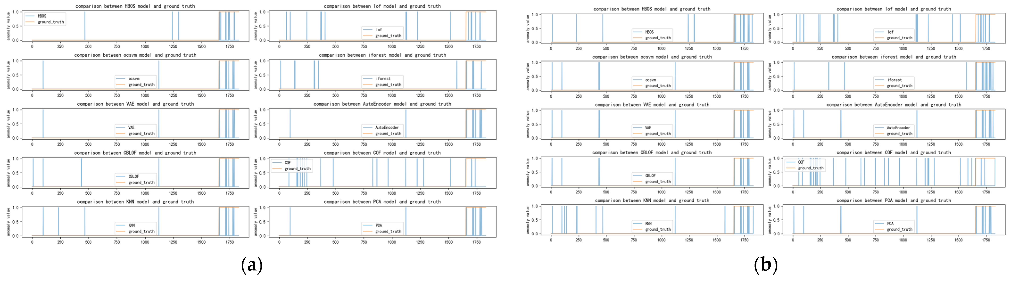
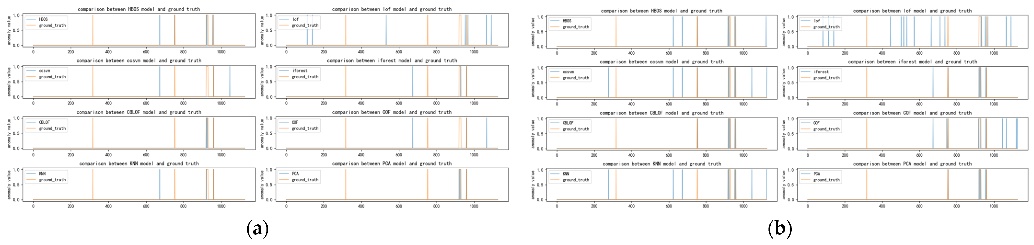
Figure 5, Figure 6, Figure 7 and Figure 8 depict the classification of anomalous labels under different time windows in the SKAB dataset. The yellow line represents the actual labels, while the blue line represents the anomaly labels generated by each detector within a fixed number of anomalies. From the figures, it is evident that almost every basic detector exhibits some false alarms and omissions in anomaly detection.
By comparing the extent of overlap between the yellow region (actual anomalies) and the blue region (detected anomalies), we can assess the performance of different detectors. Figure 5 demonstrates that it is challenging to determine which detectors are better suited for integration when the time window is small. And our algorithm also judges that there are multiple detectors focused on some data points, making it difficult to choose.
As the time window continues to increase, specifically in the range of 30–60, the number of selected detectors starts to decline and becomes more concentrated. Among them, VAE and AutoEncoder consistently maintain their favorable rankings. Other anomaly detectors occasionally appear or disappear. Notably, the PCA algorithm exhibits greater stability. Figure 7 and Figure 8 further confirm that these algorithms perform well in the anomaly region. While there are other algorithms like COF and LOF that excel in detecting certain anomalies, their numbers are relatively limited compared to the selected detectors. Hence, they were not chosen for integration.
Table 6 presents the detectors selected by our algorithm with comparable performance under different time windows. Meanwhile, Table 7 displays the preferred detectors when combining multiple time windows. It is evident that the selection of detectors tends to stabilize as the number of time window combinations increases. The combination of multiple time windows effectively mitigates the impact of randomness associated with a single time window.
However, it is important to note that determining whether a larger time window is superior is not possible to conclude definitively. In datasets such as twitter and other non-cumulative data anomalies (as shown in Appendix A), employing too many time windows may not align with the actual distribution of anomalies, leading to algorithmic judgment issues. Therefore, for practical purposes, we recommend limiting the selection of time windows based on the number of actual data anomalies. Generally, it is optimal to set the time window to no more than 1.5 times the size of the actual anomaly area. This approach ensures a more accurate assessment of anomalies while avoiding potential judgment problems caused by excessive time window combinations.
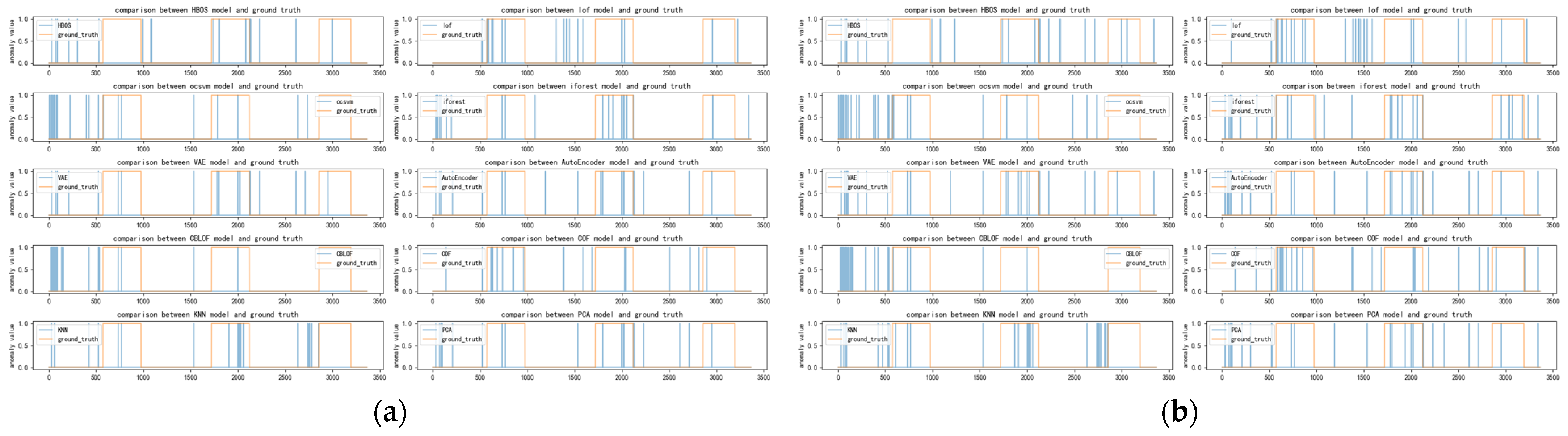
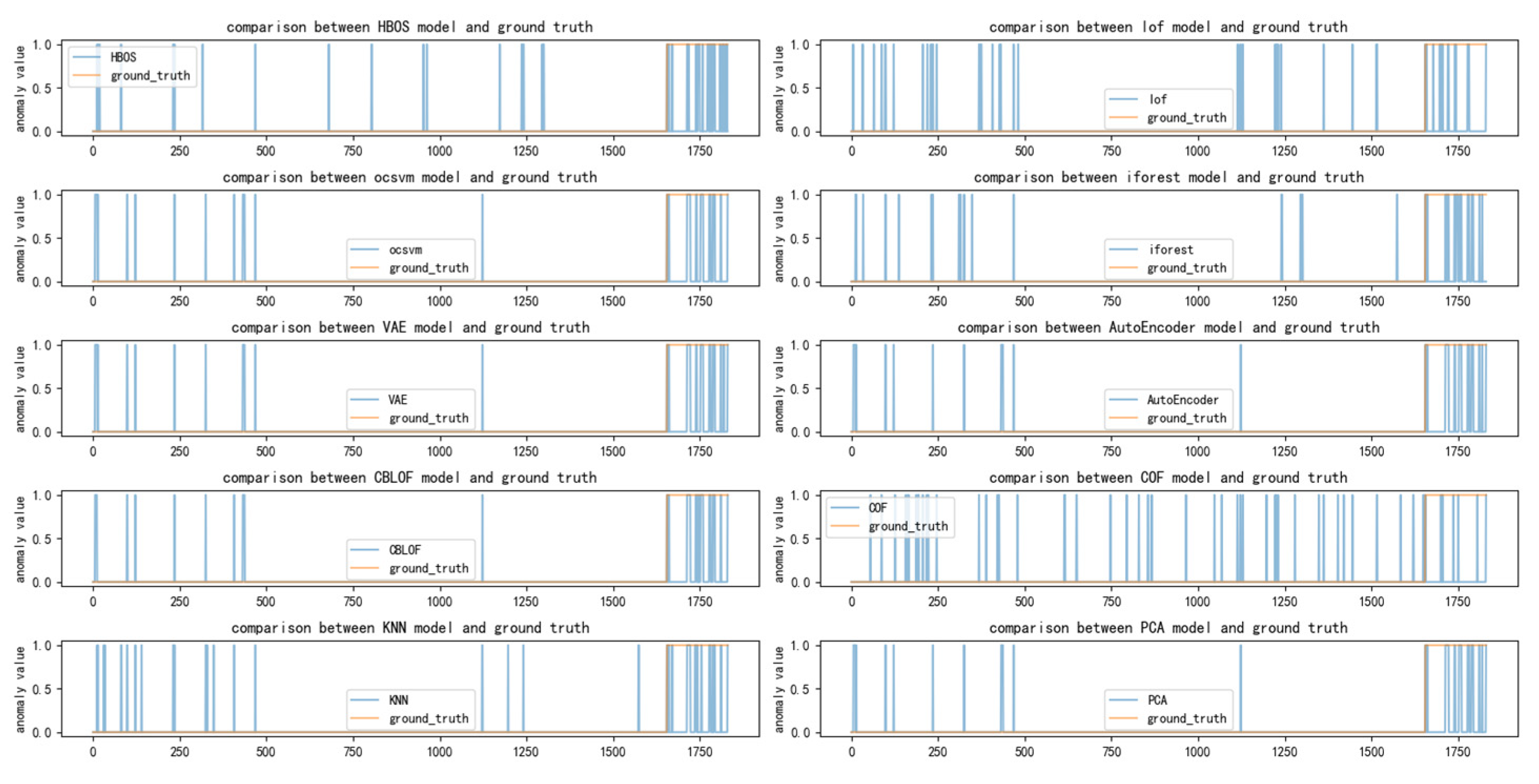
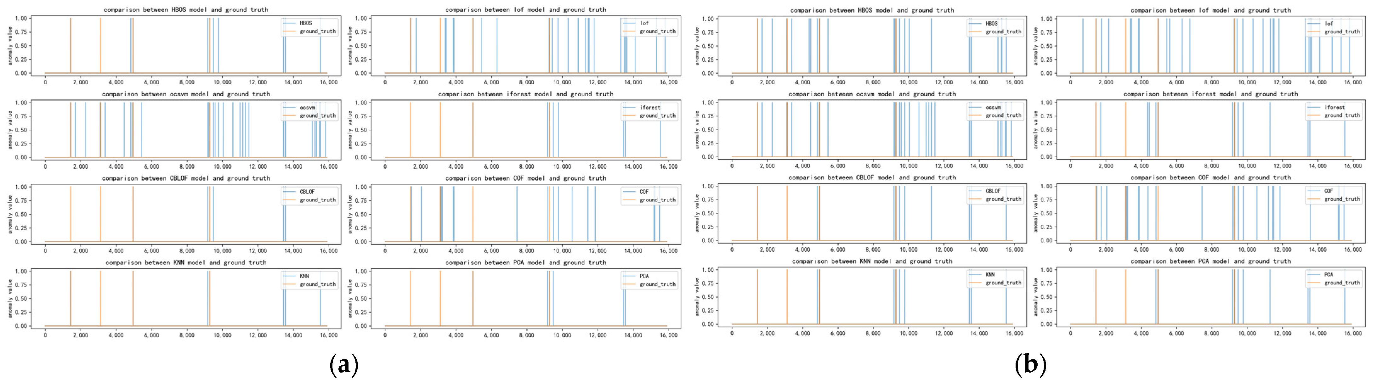
Figure 9, Figure 10, Figure 11 and Figure 12 depict the classification of anomalous labels under different time windows of the occu dataset. Table A4 presents the detectors selected by our algorithm with comparable performance under different time windows and the preferred detectors when combining multiple time windows.
As observed in Figure 9, Figure 10, Figure 11 and Figure 12, the distribution of anomalies in the occu dataset is limited, and these anomalies occur for a short duration. When the time window is small, detectors such as HBOS, OCSVM, IFOREST, CBLOF, KNN, and PCA can effectively identify these anomalies. However, as the time window increases, the accuracy of these detectors starts to decline, leading to a concentration of errors on certain common points, which results in misreported anomalies. Consequently, our method remains relatively stable regardless of changes in the time window, and different combinations of time windows do not significantly affect the preferred model’s outcomes. This is also evident from Table 8. Although our method successfully selects a few anomaly detectors that perform well, this could be attributed to chance or the specific selection of basic detectors. Our analysis suggests that this observation may be related to the characteristics of the occu dataset. All datasets from this data source are one-dimensional and exhibit a discrete distribution of anomalies. A similar pattern can be observed in the speed and twitter datasets, as outlined in Appendix A. Upon further examination of the results, when some of the underlying anomaly detectors correctly identify similar anomalies, our method can identify these detectors with similar detection results.
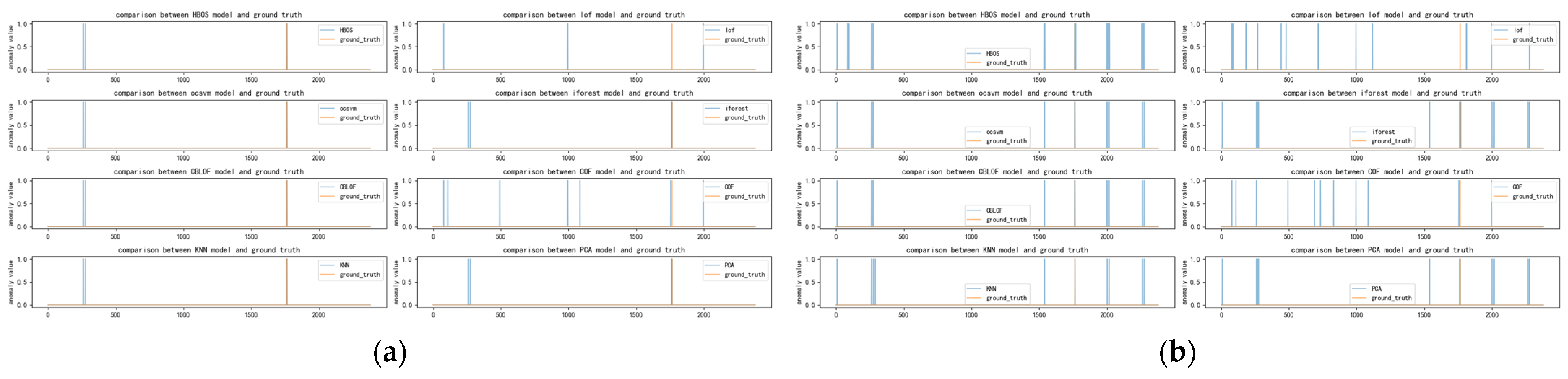
Figure 13, Figure 14, Figure 15 and Figure 16 depict the classification of anomalous labels under different time windows of the cardio dataset. Table 9 presents the detectors selected by our algorithm with comparable performance under different time windows and the preferred detectors when combining multiple time windows. The cardio dataset is characterized by the fact that its anomalies are concentrated on the last period of time and are cumulative continuous anomalies. This differs from both the SKAB and occu datasets.
As evident from the changes depicted in Figure 13, Figure 14, Figure 15 and Figure 16, most of the base detectors exhibit effective recognition of cardio anomaly data in the case of a small window setting. However, as the time window increases, sporadic false alarms of anomalies start to emerge, although the primary anomalies remain concentrated in the final segment. Nonetheless, our method adeptly selects the three detectors (VAE, AutoEncoder, PCA) that demonstrate the best recognition capability. The primary reason behind this lies in the fact that, as the time window expands, the other anomaly detectors, while also proficient at identifying true anomalies, tend to exhibit a higher tendency to falsely recognize anomalies compared to the three VAEs. Conversely, the three detectors (VAE, AutoEncoder, PCA) are better at concentrating on the actual anomalies, making them stand out. Additionally, from Figure 9 and Figure 16, it can be observed that when the time window is either too small or too large, it becomes more challenging to select our method. However, the combination of time windows can effectively address this issue and provide an appropriate solution.
It is evident that our time-window combination approach may effectively select the underlying detectors that demonstrate excellent performance in identifying cumulative anomalies over extended periods of time. This observation is further supported by the analysis of the vowels dataset in Appendix A. However, in order to consistently demonstrate this conclusion, further experiments with datasets exhibiting similar characteristics would be necessary. This is one of the future directions of this work.
It is worth highlighting that each time window experiment in this study involves separate retraining and data detection processes. The results obtained demonstrate a certain degree of reproducibility, as indicated by the variability of anomalies observed in some of the detectors shown in the figure. The majority of the detectors employed are traditional machine learning algorithms, while neural network algorithms like VAE and AutoEncoder exhibit notably consistent anomaly detection outcomes.
5.2. Comparison of Anomaly Detection Algorithms
Table 10 shows the results obtained with each dataset of the preferred algorithm scheme introduced in Section 3. Table 11, Table 12, Table 13, Table 14, Table 15, Table 16 and Table 17 show the performance of each algorithm with 7 real-world datasets. The NAB dataset is not suitable for neural network type anomaly detection algorithms due to its one-dimensional characteristics and is therefore considered in this study.
Table 11 provides clear evidence that the proposed method accurately selects three models with the highest anomaly detection performance in the SKAB dataset: PCA, AutoEncoder, and PCA (repeated entry). The integration results of these three models demonstrate optimal performance or a mere 0.1% degradation in each metric, as mentioned.
However, the performance of the proposed methods varies across the NAB datasets. Exceptional anomaly detectors were identified by our method on the ad-cpc, cardio, and vowels datasets. Additionally, our two integrated models successfully synthesized abnormal results from multiple models, resulting in improved performance compared to the basic detector. Notably, AUC, precision, recall, and F1 scores exhibited a 1–2% improvement across the different datasets.
Nevertheless, there are also some perplexing results. In the case of the cardio dataset, VAE, AutoEncoder, and PCA exhibited identical performance, which is puzzling. However, since these three algorithms were selected by the optimization model, the results of the proposed hybrid algorithm align with those of the other algorithms.
Regarding the occu and speed datasets, our method yielded only a few outstanding results. Observational indicators reveal that our method falls short of optimal performance in terms of AUC and recall. A detailed comparison of the performance of selected base detectors indicates that certain methods achieved 100% effectiveness on these datasets. However, this poses a challenge to the accuracy of the integration results, as the integration model takes into account negative outcomes from other models. Simultaneously, the high recall rate significantly impairs accuracy and F1 values. It is plausible that the choice of an anomaly threshold affects the range of identified anomalies within the data. Further research is needed to determine a reasonable threshold selection method.
In contrast, the performance metrics on the twitter dataset were the poorest. Upon analyzing the data, we discovered that the abnormal changes within the twitter dataset were abrupt, resulting in the excessive inclusion of normal data across numerous time windows. We believe that, in practical applications, the choice of the time window should be correlated with the number of detectable anomalies. This aspect requires further experimentation and investigation.
Based on this experiment, we can derive the following conclusions. Our two integration methods are designed to harmonize the anomaly results obtained from different detectors. The final results exhibit an error margin of approximately plus or minus 3% from the optimal value of the detector. Currently, we do not have a clear understanding of the decisive factors that contribute to better or worse results. At present, it appears to be a random issue. However, based on the results, our multiple time window strategy proves effective in selecting anomaly detectors that yield similar recognition outcomes. Additionally, our integration method successfully combines these detectors to produce outstanding anomaly results.
The results produced with the SKAB, cardio, and vowels datasets are visualized in Figure 17a which shows the visualization results of SKAB abnormal data, while Figure 17b visualizes the abnormal results of cardio, and Figure 17c visualizes the abnormal results of vowels. The dimensionality reduction operation of the dataset is primarily performed by the t-SNE method, and the dataset is projected onto a two-dimensional space. In the figure, the detection of abnormal points with 10 basic detectors and the 2 hybrid models proposed in this paper are repeated with points of different colors and sizes. Because other datasets are one-dimensional, and most abnormal points are outliers, no additional analysis is performed.
The visualizations of cardio and vowels show that mixed models are more advantageous in detecting local outliers clustered together. When the data have locality, the method in this paper produces better classification when recognizing outliers. However, when the data are scattered or there are multiple aggregation points, this method achieves a good recognition rate for peripheral points but fails sometimes with local points. Concurrently, the application effect of this method with the SKAB dataset is inferior to that of the other two datasets. Based on these visualizations, the proposed hybrid model can be deemed useful when the characteristics of the data appear to be aggregated.
5.3. Comparison of Integrated Methods
The data in bold in the table indicate the best performing integrated algorithm with that dataset.
The experimental results provide compelling evidence for the effectiveness of the proposed integrated method in this paper. The performance analysis on key datasets reveals both advantages and disadvantages when considering AUC. The integrated models and LSCP exhibit comparable AUC values, with minimal differences numerically. However, when evaluating precision and F1 performance, the integrated methods outperform the others. The precision-based integrated model and LSCP achieve better performances overall, except for the SKAB and speed datasets, where the precision-based integrated model performed better compared to LSCP.
On the other hand, the recall indicator is where the integrated model based on sensitivity excels. This model focuses more on identifying possible abnormal results, leading to higher recall rates. However, this process may generate numerous false alarms, resulting in lower AUC and precision values.
For the speed dataset, the effects of the three methods are similar. This outcome aligns with previous research on the speed dataset, which attributes the results to the dataset’s distinct abnormal characteristics. Consequently, the basic detector selected in the initial step is closer to its prediction results, promoting consistency in the integrated process.
5.4. Instance Validation
The anomaly detection integrated algorithm mentioned in Section 3 is used to model the data and fuse the results, which are shown in Table 22.
Experimental results show that the proposed fault diagnosis method achieves a high accuracy rate for faults that are injected into the tomcat dataset. However, the mixed model can also yield high early warning and low recall rates, which may be related to oversampling when fault data are actually labeled abnormal. When the AUC values of the two mixed models based on sensitivity and accuracy are consistent in the table, the number of models obtained by the model selection in the previous step is two, likely due to these data. When two models are selected to be fused, the data will be considered abnormal for the two integrated schemes if one model is considered abnormal. In addition, the anomaly scores are consistent; thus, the performance indicators of the two methods are consistent.
5.5. Summary of Experiments
Through experimentation, the proposed anomaly detection algorithm based on time windows achieves a good performance with multidimensional data. The algorithm can filter out multiple models that are more suitable for the dataset from multiple anomaly basic detectors and merge the results through two strategies. The algorithm can also obtain optimal or suboptimal performance results. Although its performance is mediocre on one-dimensional data, the algorithm is shown to achieve excellent performance with software fault diagnosis experimentally.
5.6. Limitations and Future Directions
First and foremost, we are unable to provide a clear explanation for the observed improvement in detection performance resulting from the choice of time window. Intuitively, we can comprehend that cumulative anomalies exhibit a gradual change in their data distribution over time until an anomaly occurs. However, the selection of multiple time windows in this study occasionally leads to the selection of a detector that may not necessarily be the best performing model. As a consequence, the final integration of anonmalous results is affected, as evidenced by its poor performance in certain datasets. The interpretability of the method presented in this paper lacks a clear intuitive explanation.
Moreover, the integration models based on precision and sensitivity present conflicting perspectives. An excessive focus on accuracy can sometimes lead to lower recall and F1 values for the method. Conversely, being overly sensitive to anomalous data can result in higher false alarm rates. The paper does not adequately address how to strike a balance between these two aspects. The consideration of this balance is not well addressed in this study.
6. Conclusions
In this study, we developed an anomaly detection integrated method based on the anomaly continuity criterion. Different from traditional combinatorial methods, this method considers the weighted statistics of each test instance in different anomaly time windows when selecting the optimal detector. Two detector-integrated methods based on accuracy and sensitivity are proposed. To verify its effectiveness, the proposed method is evaluated with seven real datasets and one real-time data collection.
The results obtained from our proposed method demonstrate the successful integration of anomaly effects, aligning with our initial expectations. In certain instances, the integrated results exhibit a high level of consistency with the outcomes obtained from the optimal detector. In the majority of cases, there is a marginal decrease of only 3% in precision, indicating a minimal impact on accuracy.
Furthermore, our proposed multiple time window strategy is specifically designed to capture the temporal characteristics of cumulative anomalies. This approach allows for a more effective extraction of the distribution of anomaly data. By targeting these temporal aspects, our method enhances the ability to accurately identify and analyze cumulative anomalies.
These findings highlight the efficacy of our approach in achieving consistent and accurate anomaly detection results. The integration of anomaly effects and the utilization of the multiple time window strategy contribute to a comprehensive understanding of the anomalies, leading to improved detection performance. The minimal decrease in precision further demonstrates the robustness and reliability of our proposed method.
Author Contributions
Conceptualization, T.S., J.A. and Z.Z.; methodology, T.S., J.A. and Z.Z.; software, T.S. and Z.Z.; validation, T.S. and Z.Z.; investigation, Z.Z. and T.S.; resources, T.S.; data curation, T.S.; writing—original draft preparation, T.S. and Z.Z.; writing—review and editing, T.S., J.A. and Z.Z.; visualization, T.S.; supervision, J.A.; project administration, J.A. All authors have read and agreed to the published version of the manuscript.
Funding
This research received no external funding.
Institutional Review Board Statement
Not applicable.
Informed Consent Statement
Not applicable.
Data Availability Statement
The source code of the method implementation can be downloaded at (https://gitee.com/stlinger/anomaly-detection-Integrated-model, accessed on 10 August 2023). The publicly available dataset used for the anomaly detection task can be found downloaded at [32,33] (https://github.com/waico/SkAB, and https://github.com/numenta/NAB, accessed on 1 October 2023).
Acknowledgments
The authors would like to thank the editors and anonymous reviewers for their constructive comments and suggestions for improving this work.
Conflicts of Interest
The authors declare no conflict of interest.
Appendix A
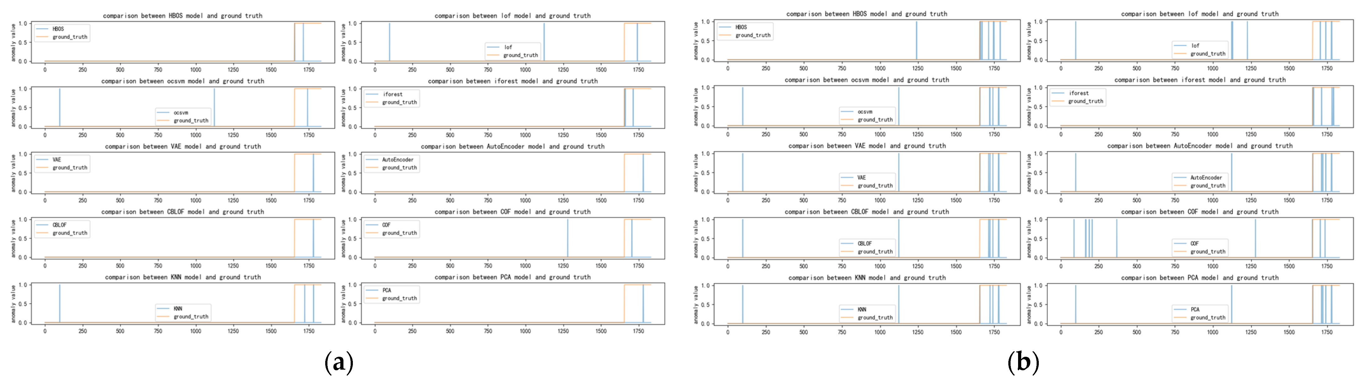
The experimental data and graphs for the remaining four datasets in Experimental Section 5.1 are shown here. Figure A1, Figure A2, Figure A3 and Figure A4 depict the classification of anomalous labels under different time windows in the SKAB dataset. Table A1 presents the detectors selected by our algorithm with comparable performance under different time windows and the preferred detectors when combining multiple time windows.
Figure A1.
(a) Distribution of anomalies with a time window of two for ad-cpc dataset; (b) Distribution of anomalies with a time window of ten for ad-cpc dataset.
Figure A1.
(a) Distribution of anomalies with a time window of two for ad-cpc dataset; (b) Distribution of anomalies with a time window of ten for ad-cpc dataset.

Figure A2.
(a) Distribution of anomalies with a time window of 20 for ad-cpc dataset; (b) Distribution of anomalies with a time window of 30 for ad-cpc dataset.
Figure A2.
(a) Distribution of anomalies with a time window of 20 for ad-cpc dataset; (b) Distribution of anomalies with a time window of 30 for ad-cpc dataset.

Figure A3.
(a) Distribution of anomalies with a time window of 40 for ad-cpc dataset; (b) Distribution of anomalies with a time window of 50 for ad-cpc dataset.
Figure A3.
(a) Distribution of anomalies with a time window of 40 for ad-cpc dataset; (b) Distribution of anomalies with a time window of 50 for ad-cpc dataset.

Figure A4.
Distribution of anomalies with a time window of 60 for ad-cpc dataset.


Table A1.
Algorithm selection result under different time windows for ad-cpc dataset.
| Size of Time Windows | Detector of Choice | Time Widow Combination | Detector of Choice |
|---|---|---|---|
| 2 | LOF, COF | 2-10 | LOF, COF, |
| 10 | LOF, COF, | 2-20 | LOF, COF, |
| 20 | LOF, COF, IFOREST, KNN | 2-30 | LOF, COF |
| 30 | LOF, COF, KNN PCA | 2-40 | LOF, COF, KNN |
| 40 | LOF, COF, KNN | 2-50 | LOF, COF, KNN |
| 50 | LOF, COF, KNN | 2-60 | LOF, COF, KNN |
| 60 | LOF, COF, KNN |
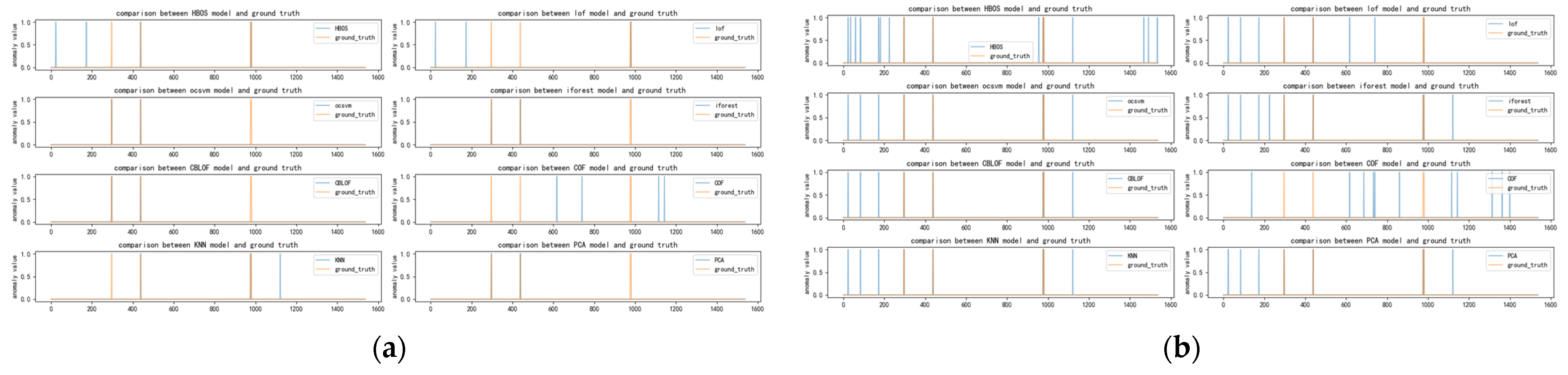
The ap-cpc dataset exhibits similar characteristics to the occu dataset, featuring a higher number of anomalies, albeit with short durations. The eight base detectors applied to the speed dataset produce comparable detection results. With a small time window, each detector primarily identifies a single anomaly. As the time window expands, the number of correct detections of anomalies increases proportionally with the number of false detections. In contrast, our preferred method is less susceptible to variations in the time window, particularly when the time window is large, showing minimal changes. The experimental findings obtained from the ap-cpc dataset align with those of the occu dataset, reinforcing the consistency of the conclusions.
Figure A5, Figure A6, Figure A7 and Figure A8 depict the classification of anomalous labels under different time windows in the speed dataset. Table A2 presents the detectors selected by our algorithm with comparable performance under different time windows and the preferred detectors when combining multiple time windows.
Figure A5.
(a) Distribution of anomalies with a time window of two for speed dataset; (b) Distribution of anomalies with a time window of ten for speed dataset.
Figure A5.
(a) Distribution of anomalies with a time window of two for speed dataset; (b) Distribution of anomalies with a time window of ten for speed dataset.

Figure A6.
(a) Distribution of anomalies with a time window of 20 for speed dataset; (b) Distribution of anomalies with a time window of 30 for speed dataset.
Figure A6.
(a) Distribution of anomalies with a time window of 20 for speed dataset; (b) Distribution of anomalies with a time window of 30 for speed dataset.

Figure A7.
(a) Distribution of anomalies with a time window of 40 for speed dataset; (b) Distribution of anomalies with a time window of 50 for speed dataset.
Figure A7.
(a) Distribution of anomalies with a time window of 40 for speed dataset; (b) Distribution of anomalies with a time window of 50 for speed dataset.

Figure A8.
Distribution of anomalies with a time window of 60 for speed dataset.

Table A2.
Algorithm selection result under different time windows for speed dataset.
| Size of Time Windows | Detector of Choice | Time Widow Combination | Detector of Choice |
|---|---|---|---|
| 2 | HBOS, OCSVM, IFOREST, CBLOF, COF, KNN, PCA | 2-10 | HBOS, IFOREST, CBLOF, PCA |
| 10 | HBOS, IFOREST, CBLOF, PCA | 2-20 | HBOS, IFOREST, CBLOF, PCA |
| 20 | HBOS, IFOREST, CBLOF, PCA | 2-30 | HBOS, IFOREST, CBLOF, PCA |
| 30 | HBOS, IFOREST, CBLOF, PCA | 2-40 | HBOS, IFOREST, CBLOF, PCA |
| 40 | HBOS, IFOREST, CBLOF, KNN, PCA | 2-50 | HBOS, IFOREST, CBLOF, PCA |
| 50 | HBOS, IFOREST, CBLOF, KNN, PCA | 2-60 | HBOS, IFOREST, CBLOF, PCA |
| 60 | HBOS, OCSVM, IFOREST, CBLOF, KNN, PCA |
The experimental findings on the speed dataset exhibit remarkable similarities to the occu dataset. As depicted in Table A2, it is evident that our selection method is not as effective on this particular dataset, despite successfully selecting the four detectors with the best performance.
Figure A9, Figure A10, Figure A11 and Figure A12 depict the classification of anomalous labels under different time windows in the twitter dataset. Table A3 presents the detectors selected by our algorithm with comparable performance under different time windows and the preferred detectors when combining multiple time windows.
Figure A9.
(a) Distribution of anomalies with a time window of two for twitter dataset; (b) Distribution of anomalies with a time window of ten for twitter dataset.
Figure A9.
(a) Distribution of anomalies with a time window of two for twitter dataset; (b) Distribution of anomalies with a time window of ten for twitter dataset.

Figure A10.
(a) Distribution of anomalies with a time window of 20 for twitter dataset; (b) Distribution of anomalies with a time window of 30 for twitter dataset.
Figure A10.
(a) Distribution of anomalies with a time window of 20 for twitter dataset; (b) Distribution of anomalies with a time window of 30 for twitter dataset.

Figure A11.
(a) Distribution of anomalies with a time window of 40 for twitter dataset; (b) Distribution of anomalies with a time window of 50 for twitter dataset.
Figure A11.
(a) Distribution of anomalies with a time window of 40 for twitter dataset; (b) Distribution of anomalies with a time window of 50 for twitter dataset.

Figure A12.
Distribution of anomalies with a time window of 60 for twitter dataset.

Table A3.
Algorithm selection result under different time windows for twitter dataset.
| Size of Time Windows | Detector of Choice | Time Widow Combination | Detector of Choice |
|---|---|---|---|
| 2 | HBOS, OCSVM, IFOREST, CBLOF, KNN, PCA | 2-10 | HBOS, OCSVM, IFOREST, CBLOF, PCA |
| 10 | HBOS, OCSVM, IFOREST, CBLOF, PCA | 2-20 | HBOS, OCSVM, IFOREST, CBLOF, PCA |
| 20 | HBOS, OCSVM, IFOREST, CBLOF, PCA | 2-30 | HBOS, OCSVM, CBLOF |
| 30 | HBOS, OCSVM, CBLOF | 2-40 | HBOS, OCSVM, CBLOF |
| 40 | HBOS, OCSVM, CBLOF | 2-50 | HBOS, OCSVM, CBLOF |
| 50 | HBOS, OCSVM, CBLOF, KNN | 2-60 | HBOS, OCSVM, CBLOF |
| 60 | HBOS, OCSVM, CBLOF, KNN |
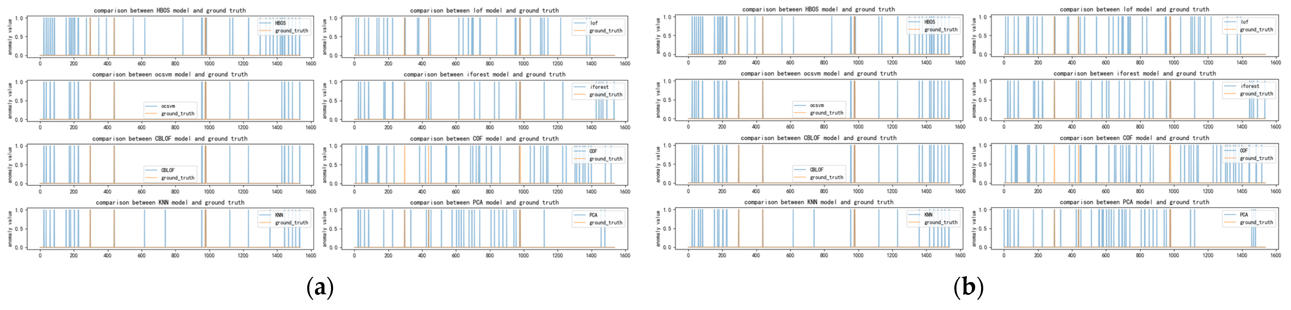
The twitter dataset, sourced from the NAB data source, exhibits anomaly characteristics that are essentially the same as those of the occu, speed, and other datasets, as depicted in Figure A9, Figure A10, Figure A11 and Figure A12. These figures clearly illustrate the anomaly detection results of each detector. Notably, OCSVM, LOF, and COF display prominent false alarm rates, while HBOS, CBLOF, IFOREST, and PCA exhibit more similar results. However, our method ultimately selects OCSVM, HBOS, and CBLOF, which may appear puzzling at first glance.
Upon closer inspection, it becomes evident that the twitter dataset contains a significantly larger amount of data compared to the other datasets. Although it might seem that OCSVM should have more overlap with LOF, COF, and other detectors based on the graphs, in reality, the overlap is not as substantial as it appears, possibly due to the effects of shrinkage. The concentration of true anomalies emerges as the crucial factor in selecting an anomaly detector. However, this concentration is also a side effect of using a large time window for discrete anomalies.
Figure A13, Figure A14, Figure A15 and Figure A16 depict the classification of anomalous labels under different time windows in the vowels dataset. Table A4 presents the detectors selected by our algorithm with comparable performance under different time windows and the preferred detectors when combining multiple time windows.
Figure A13.
(a) Distribution of anomalies with a time window of two for vowels dataset; (b) Distribution of anomalies with a time window of ten for vowels dataset.
Figure A13.
(a) Distribution of anomalies with a time window of two for vowels dataset; (b) Distribution of anomalies with a time window of ten for vowels dataset.

Figure A14.
(a) Distribution of anomalies with a time window of 20 for twitter dataset; (b) Distribution of anomalies with a time window of 30 for vowels dataset.
Figure A14.
(a) Distribution of anomalies with a time window of 20 for twitter dataset; (b) Distribution of anomalies with a time window of 30 for vowels dataset.

Figure A15.
(a) Distribution of anomalies with a time window of 40 for vowels dataset; (b) Distribution of anomalies with a time window of 50 for vowels dataset.
Figure A15.
(a) Distribution of anomalies with a time window of 40 for vowels dataset; (b) Distribution of anomalies with a time window of 50 for vowels dataset.

Figure A16.
Distribution of anomalies with a time window of 60 for vowels dataset.

Table A4.
Algorithm selection result under different time windows for vowels dataset.
| Size of Time Windows | Detector of Choice | Time Widow Combination | Detector of Choice |
|---|---|---|---|
| 2 | LOF, IFOREST, KNN | 2-10 | IFOREST, KNN |
| 10 | IFOREST, CBLOF, KNN | 2-20 | LOF, IFOREST, CBLOF, KNN |
| 20 | LOF, OCSVM, CBLOF, COF, KNN | 2-30 | LOF, CBLOF, KNN |
| 30 | LOF, CBLOF, KNN | 2-40 | LOF, CBLOF, COF, KNN |
| 40 | LOF, CBLOF, COF, KNN | 2-50 | LOF, CBLOF, KNN |
| 50 | LOF, CBLOF, KNN | 2-60 | LOF, CBLOF, KNN |
| 60 | LOF, OCSVM, CBLOF, COF, KNN |
The vowels dataset is a multidimensional dataset that shares similarities with the cardio dataset. As the time window increases, the figures indicate that the results of each detector begin to concentrate in different regions. Detectors with scattered anomaly results are eliminated, while those exhibiting concentration in a particular region, regardless of correct or incorrect anomalies, are selected. The different time windows also influence the final detector selection. Although the selection results tend to stabilize with LOF, CBLOF, and KNN, there are occasional instances where other detectors are chosen. It is evident that our method is not yet fully stable on this dataset, as observed from the fluctuating selection outcomes.
References
- Wong, W.E.; Li, X.; Laplante, P.A. Be more familiar with our enemies and pave the way forward: A review of the roles bugs played in software failures. J. Syst. Softw. 2017, 133, 68–94. [Google Scholar]
- Newman, M. Software Errors Cost US Economy $59.5 Billion Annually, NIST Assesses Technical Needs of Industry to Improve Software-Testing. 2002. Available online: https://www.nist.gov/system/files/documents/director/planning/report02-3.pdf (accessed on 5 April 2023).
- Zhao, Y.; Nasrullah, Z.; Li, Z. PyOD: A Python Toolbox for Scalable Outlier Detection. arXiv 2019, arXiv:1901.01588. [Google Scholar]
- Zhao, G.; Hassan, S.; Zou, Y.; Truong, D.; Corbin, T. Predicting Performance Anomalies in Software Systems at Run-time. ACM Trans. Softw. Eng. Methodol. 2021, 30, 1–33. [Google Scholar] [CrossRef]
- Kohyarnejadfard, I.; Aloise, D.; Dagenais, M.R.; Shakeri, M. A Framework for Detecting System Performance Anomalies Using Tracing Data Analysis. Entropy 2021, 23, 1011. [Google Scholar] [CrossRef] [PubMed]
- Guggilam, S.; Chandola, V.; Patra, A. Tracking clusters and anomalies in evolving data streams. Stat. Anal. Data Mining ASA Data Sci. J. 2022, 15, 156–178. [Google Scholar] [CrossRef]
- Luo, Y.; Ben, K. Summary of Software Failure Static Prediction Methods. Comput. Sci. Explor. 2009, 3, 449–459. [Google Scholar]
- Khoshgoftaar, T.M.; Gao, K. Count Models for Software Quality Estimation. IEEE Trans. Reliab. 2007, 56, 212–222. [Google Scholar] [CrossRef]
- Gao, K.; Khoshgoftaar, T.M. A Comprehensive Empirical Study of Count Models for Software Fault Prediction. IEEE Trans. Reliab. 2007, 56, 223–236. [Google Scholar] [CrossRef]
- Janes, A.; Scotto, M.; Pedrycz, W.; Russo, B.; Stefanovic, M.; Succi, G. Identification of defect-prone classes in telecommunication software systems using design metrics. Inf. Sci. 2006, 176, 3711–3734. [Google Scholar] [CrossRef]
- Menzies, T.; Greenwald, J.; Frank, A. Data Mining Static Code Attributes to Learn Defect Predictors. IEEE Trans. Softw. Eng. 2007, 33, 2–13. [Google Scholar] [CrossRef]
- Jia, S.; Hou, C.; Wang, J. Software aging analysis and prediction in a web server based on multiple linear regression algorithm. In Proceedings of the 2017 IEEE 9th International Conference on Communication Software and Networks (ICCSN), Guangzhou, China, 6–8 May 2017; pp. 1452–1456. [Google Scholar] [CrossRef]
- Cotroneo, D.; Natella, R.; Pietrantuono, R. Predicting aging-related bugs using software complexity metrics. Perform. Evaluation 2013, 70, 163–178. [Google Scholar] [CrossRef]
- Cinque, M.; Cotroneo, D.; Della Corte, R.; Pecchia, A. A framework for on-line timing error detection in software systems. Futur. Gener. Comput. Syst. 2019, 90, 521–538. [Google Scholar] [CrossRef]
- Arning, A.; Agrawal, R.; Raghavan, P. A Linear Method for Deviation Detection in Large Databases. United States: N. p., 1996. Web. Available online: https://cdn.aaai.org/KDD/1996/KDD96-027.pdf (accessed on 5 April 2023).
- Schölkopf, B.; Platt, J.C.; Shawe-Taylor, J.; Smola, A.J.; Williamson, R.C. Estimating the Support of a High-Dimensional Distribution. Neural Comput. 2001, 13, 1443–1471. [Google Scholar] [CrossRef]
- Shyu, M.; Chen, S.; Sarinnapakorn, K.; Chang, L. A novel anomaly detection scheme based on principal component classifier. In Proceedings of the IEEE Foundations and New Directions of Data Mining Workshop, in conjunction with the Third IEEE International Conference on Data Mining, ICDM’03, 2003, pp. 172–179. Available online: https://scholar.google.com.hk/scholar?hl=en&as_sdt=0%2C5&q=.+A+novel+anomaly+detection+scheme+based+on+principal+component+classifier.+&btnG=#d=gs_cit&t=1696759862460&u=%2Fscholar%3Fq%3Dinfo%3AjiTPoAYrCo8J%3Ascholar.google.com%2F%26output%3Dcite%26scirp%3D0%26hl%3Den (accessed on 5 April 2023).
- Ramaswamy, S.; Rastogi, R.; Shim, K. Efficient algorithms for mining outliers from large data sets. In Proceedings of the 2000 ACM SIGMOD International Conference on Management of Data, New York, NY, USA, 15–18 May 2000; pp. 427–438. [Google Scholar] [CrossRef]
- Angiulli, F.; Pizzuti, C. Fast Outlier Detection in High Dimensional Spaces. In European Conference on Principles of Data Mining and Knowledge Discovery; Springer: Berlin/Heidelberg, Germany, 2002; Volume 2431, pp. 15–27. [Google Scholar] [CrossRef]
- Breunig, M.M.; Kriegel, H.-P.; Ng, R.T.; Sander, J. LOF: Identifying Density-Based Local Outliers. In Proceedings of the 2000 ACM SIGMOD International Conference on Management of Data, Association for Computing Machinery, New York, NY, USA, 16–18 May 2000; pp. 93–104. [Google Scholar] [CrossRef]
- Tang, J.; Chen, Z.; Fu, A.W.; Cheung, D.W. Enhancing Effectiveness of Outlier Detections for Low Density Patterns. In Advances in Knowledge Discovery and Data Mining; Springer: Berlin/Heidelberg, Germany, 2002; pp. 535–548. [Google Scholar] [CrossRef]
- He, Z.; Xu, X.; Deng, S. Discovering cluster-based local outliers. Pattern Recognit. Lett. 2003, 24, 1641–1650. [Google Scholar] [CrossRef]
- Goldstein, M.; Dengel, A. Histogram-based Outlier Score (HBOS): A fast Unsupervised Anomaly Detection Algorithm. KI-2012 Poster Demo Track 2012, 1, 59–63. [Google Scholar]
- Almardeny, Y.; Boujnah, N.; Cleary, F. A Novel Outlier Detection Method for Multivariate Data. IEEE Trans. Knowl. Data Eng. 2020, 34, 4052–4062. [Google Scholar] [CrossRef]
- Kingma, D.P.; Welling, M. Auto-Encoding Variational Bayes. arXiv 2013, arXiv:1312.6114. Available online: http://arxiv.org/abs/1312.6114 (accessed on 2 September 2021).
- YLiu, Y.; Li, Z.; Zhou, C.; Jiang, Y.; Sun, J.; Wang, M.; He, X. Generative Adversarial Active Learning for Unsupervised Outlier Detection. IEEE Trans. Knowl. Data Eng. 2020, 32, 1517–1528. [Google Scholar] [CrossRef]
- Blázquez-García, A.; Conde, A.; Mori, U.; Lozano, J.A. A Review on Outlier/Anomaly Detection in Time Series Data. ACM Comput. Surv. 2021, 54, 1–33. [Google Scholar] [CrossRef]
- Chatterjee, A.; Ahmed, B.S. IoT anomaly detection methods and applications: A survey. Internet Things 2022, 19, 100568. [Google Scholar] [CrossRef]
- Oreilly, C.; Gluhak, A.; Imran, M.A. Distributed Anomaly Detection Using Minimum Volume Elliptical Principal Component Analysis. IEEE Trans. Knowl. Data Eng. 2016, 28, 2320–2333. [Google Scholar] [CrossRef]
- Zhao, Y.; Nasrullah, Z.; Hryniewicki, M.K.; Li, Z. LSCP: Locally Selective Combination in Parallel Outlier Ensembles. In Proceedings of the 2019 SIAM International Conference on Data Mining; Society for Industrial and Applied Mathematics: Philadelphia, PA, USA, 2019; p. 9. [Google Scholar]
- Zhao, Y.; Hu, X.; Cheng, C.; Wang, C.; Wan, C.; Wang, W.; Akoglu, L. SUOD: Accelerating Large-scale Unsupervised Heterogeneous Outlier Detection. Proc. Mach. Learn. Syst. 2021, 3, 463–478. [Google Scholar]
- Available online: https://github.com/waico/SkAB (accessed on 8 May 2023).
- Available online: https://github.com/numenta/NAB (accessed on 8 May 2023).
Figure 1.
Overall detection scheme.

Figure 2.
Automatic selection model.

Figure 3.
Time window loop.

Figure 4.
Random adjacent space.

Figure 5.
(a) Distribution of anomalies with a time window of 2 for SKAB dataset; (b) Distribution of anomalies with a time window of 10 for SKAB dataset.
Figure 5.
(a) Distribution of anomalies with a time window of 2 for SKAB dataset; (b) Distribution of anomalies with a time window of 10 for SKAB dataset.

Figure 6.
(a) Distribution of anomalies with a time window of 20 for SKAB dataset; (b) Distribution of anomalies with a time window of 30 for SKAB dataset.
Figure 6.
(a) Distribution of anomalies with a time window of 20 for SKAB dataset; (b) Distribution of anomalies with a time window of 30 for SKAB dataset.

Figure 7.
(a) Distribution of anomalies with a time window of 40 for SKAB dataset; (b) Distribution of anomalies with a time window of 50 for SKAB dataset.
Figure 7.
(a) Distribution of anomalies with a time window of 40 for SKAB dataset; (b) Distribution of anomalies with a time window of 50 for SKAB dataset.

Figure 8.
Distribution of anomalies with a time window of 60 for SKAB dataset.

Figure 9.
(a) Distribution of anomalies with a time window of two for occu dataset; (b) Distribution of anomalies with a time window of ten for occu dataset.
Figure 9.
(a) Distribution of anomalies with a time window of two for occu dataset; (b) Distribution of anomalies with a time window of ten for occu dataset.

Figure 10.
(a) Distribution of anomalies with a time window of 20 for occu dataset; (b) Distribution of anomalies with a time window of 30 for occu dataset.
Figure 10.
(a) Distribution of anomalies with a time window of 20 for occu dataset; (b) Distribution of anomalies with a time window of 30 for occu dataset.

Figure 11.
(a) Distribution of anomalies with a time window of 40 for occu dataset; (b) Distribution of anomalies with a time window of 50 for occu dataset.
Figure 11.
(a) Distribution of anomalies with a time window of 40 for occu dataset; (b) Distribution of anomalies with a time window of 50 for occu dataset.

Figure 12.
Distribution of anomalies with a time window of 60 for occu dataset.

Figure 13.
(a) Distribution of anomalies with a time window of two for cardio dataset; (b) Distribution of anomalies with a time window of ten for cardio dataset.
Figure 13.
(a) Distribution of anomalies with a time window of two for cardio dataset; (b) Distribution of anomalies with a time window of ten for cardio dataset.

Figure 14.
(a) Distribution of anomalies with a time window of 20 for cardio dataset; (b) Distribution of anomalies with a time window of 30 for cardio dataset.
Figure 14.
(a) Distribution of anomalies with a time window of 20 for cardio dataset; (b) Distribution of anomalies with a time window of 30 for cardio dataset.

Figure 15.
(a) Distribution of anomalies with a time window of 40 for cardio dataset; (b) Distribution of anomalies with a time window of 50 for cardio dataset.
Figure 15.
(a) Distribution of anomalies with a time window of 40 for cardio dataset; (b) Distribution of anomalies with a time window of 50 for cardio dataset.

Figure 16.
Distribution of anomalies with a time window of 60 for cardio dataset.

Figure 17.
(a) t-SNE visualizations on SKAB; (b) t-SNE visualizations on cardio; (c) t-SNE visualizations on vowels.
Figure 17.
(a) t-SNE visualizations on SKAB; (b) t-SNE visualizations on cardio; (c) t-SNE visualizations on vowels.

Table 1.
Abnormal data monitoring algorithm table.
| Algorithm Type | Abbreviation | Introduction |
|---|---|---|
| Linear model | PCA | Principal Component Analysis (the sum of weighted projected distances to the eigenvector hyperplanes) |
| Linear model | OCSVM | One-Class Support Vector Machines |
| Based on proximity | LOF | Local Outlier Factor |
| Based on proximity | COF | Connectivity-Based Outlier Factor |
| Based on proximity | CBLOF | Clustering-Based Local Outlier Factor |
| Based on proximity | HBOS | Histogram-based Outlier Score |
| Based on proximity | KNN | k Nearest Neighbors (use the distance to the kth nearest neighbor as the outlier score) |
| Combination of abnormal | IForest | Isolation Forest |
| Neural network | AutoEncoder | Fully connected AutoEncoder (use reconstruction error as the outlier score) |
| Neural network | VAE | Variational AutoEncoder (use reconstruction error as the outlier score) |
Table 2.
Real-world datasets used for training.
| Name | Dimension | %Outlier | Source |
|---|---|---|---|
| SKAB | (3368, 8) | 0.3385 | SKAB |
| Ad-cpc | (1538, 1) | 0.0052 | NAB |
| Occu | (2380, 1) | 0.0004 | NAB |
| speed | (1127, 1) | 0.0151 | NAB |
| (15,902, 1) | 0.003 | NAB | |
| cardio | (1831, 21) | 0.0961 | ODDS |
| vowels | (1456, 12) | 0.0343 | DAMI |
Table 3.
Real-world datasets used for validation.
| Name | Dimension | %Outlier | Source |
|---|---|---|---|
| SKAB | (2244, 8) | 0.3356 | SKAB |
| Ad-cpc | (1643, 1) | 0.0018 | NAB |
| Occu | (2500, 1) | 0.0048 | NAB |
| speed | (2495, 1) | 0.0020 | NAB |
| (15,831, 1) | 0.0013 | NAB | |
| cardio | (1730, 21) | 0.0936 | ODDS |
| vowels | (1563, 12) | 0.0275 | DAMI |
Table 4.
Parameter use of the basic anomaly detectors.
| Detector | Parameters | Value | Detector | Parameters | Value |
|---|---|---|---|---|---|
| HBOS | n_bin | 10 | OCSVM | degree | 2 |
| alpha | 0.1 | Coef0 | 0 | ||
| Tol | 0.5 | tol | 0.005 | ||
| contamination | 0.1 | nu | 0.5 | ||
| LOF | n-neighbors | 10 | contamination | 0.1 | |
| leaf_size | 15 | VAE | encoder_neurons | [15, 8, 4] | |
| contamination | 0.1 | encoder_neurons | [4, 8, 15] | ||
| p | 2 | KNN | contamination | 0.1 | |
| IFOREST | n_estimator | 10 | n-neighbors | 5 | |
| contamination | 0.1 | radius | 1.0 | ||
| max_features | 0.5 | leaf_size | 30 | ||
| n_jobs | 1 | p | 2 | ||
| AutoEncoder | hidden_neurous | [8, 15] | COF | contamination | 0.1 |
| CBLOF | n_cluster | 10 | n-neighbors | 6 | |
| contamination | 0.1 | PCA | contamination | 0.1 | |
| alpha | 0.9 | n_components | None | ||
| beta | 5 | other | default |
Table 5.
Data characteristics of tomcat failure.
| Name | Dimension | %Outlier |
|---|---|---|
| tomcat failure | 1600, 30 | 0.077 |
Table 6.
Algorithm selection results under different time windows.
| Size of Time Windows | Detector of Choice |
|---|---|
| 2 | LOF, VAE, AutoEncoder, CBLOF, KNN, PCA |
| 10 | LOF, OCSVM, VAE, AutoEncoder, CBLOF, COF, KNN, PCA |
| 20 | HBOS, OCSVM, IFOREST, VAE, AutoEncoder, CBLOF, PCA |
| 30 | IFOREST, VAE, AutoEncoder, PCA |
| 40 | VAE, AutoEncoder |
| 50 | VAE, AutoEncoder, PCA |
| 60 | SO_GAAL, VAE, AutoEncoder, CBLOF |
Table 7.
Algorithm selection results under different Time Window Combination.
| Time Widow Combination | Detector of Choice |
|---|---|
| 2-10 | LOF, VAE, AutoEncoder, CBLOF, KNN, PCA |
| 2-20 | LOF, VAE, AutoEncoder, CBLOF, PCA |
| 2-30 | LOF, VAE, AutoEncoder, PCA |
| 2-40 | VAE, AutoEncoder, PCA |
| 2-50 | VAE, AutoEncoder, PCA |
| 2-60 | VAE, AutoEncoder, PCA |
Table 8.
Algorithm selection results under different time windows of occu dataset.
| Size of Time Windows | Detector of Choice | Time Widow Combination | Detector of Choice |
|---|---|---|---|
| 2 | HBOS, OCSVM, IFOREST, CBLOF, KNN, PCA | 2-10 | HBOS, OCSVM, IFOREST, CBLOF, KNN |
| 10 | HBOS, OCSVM, IFOREST, CBLOF, KNN | 2-20 | HBOS, OCSVM, IFOREST, CBLOF, KNN |
| 20 | HBOS, OCSVM, IFOREST, CBLOF, KNN | 2-30 | HBOS, OCSVM, IFOREST, CBLOF, KNN |
| 30 | HBOS, OCSVM, IFOREST, CBLOF, KNN | 2-40 | HBOS, OCSVM, IFOREST, CBLOF, KNN |
| 40 | HBOS, OCSVM, IFOREST, CBLOF, KNN | 2-50 | HBOS, OCSVM, IFOREST, CBLOF, KNN |
| 50 | HBOS, OCSVM, IFOREST, CBLOF, KNN, PCA | 2-60 | HBOS, OCSVM, IFOREST, CBLOF, KNN |
| 60 | HBOS, OCSVM, IFOREST, CBLOF, KNN, PCA |
Table 9.
Algorithm selection results under different time windows for cardio dataset.
| Size of Time Windows | Detector of Choice | Time Widow Combination | Detector of Choice |
|---|---|---|---|
| 2 | AutoEncoder, CBLOF, KNN, PCA | 2-10 | AutoEncoder, CBLOF, KNN, PCA |
| 10 | OCSVM, VAE, AutoEncoder, CBLOF, KNN, PCA | 2-20 | VAE, AutoEncoder, PCA |
| 20 | VAE, AutoEncoder, PCA | 2-30 | VAE, AutoEncoder, PCA |
| 30 | VAE, AutoEncoder, PCA | 2-40 | VAE, AutoEncoder, PCA |
| 40 | OCSVM, IFOREST, VAE, AutoEncoder, PCA | 2-50 | VAE, AutoEncoder, PCA |
| 50 | VAE, AutoEncoder, CBLOF, KNN, PCA | 2-60 | AutoEncoder, CBLOF, KNN, PCA |
| 60 | OCSVM, VAE, AutoEncoder, CBLOF, KNN, PCA |
Table 10.
Algorithm selection result with seven datasets.
| Dataset | Algorithm of Choice |
|---|---|
| SKAB | VAE, AutoEncoder, PCA |
| Ad-cpc | LOF, COF, KNN |
| Occu | HBOS, OCSVM, CBLOF, IFOREST, KNN |
| speed | HBOS, IFOREST, CBLOF, PCA |
| OCSVM, HBO, CBLOF | |
| cardio | VAE, AutoEncoder, PCA |
| vowels | LOF, CBLOF, KNN |
Table 11.
Performance of each algorithm with the SKAB dataset.
| SKAB | mixModel-pre | mixModel-sen | HBOS | lof | OCSVM | iforest | VAE | AutoEncoder | CBLOF | COF | KNN | PCA |
|---|---|---|---|---|---|---|---|---|---|---|---|---|
| AUC | 0.6645 | 0.6638 | 0.6171 | 0.5136 | 0.5279 | 0.6058 | 0.6631 | 0.6682 | 0.4843 | 0.4531 | 0.5099 | 0.6611 |
| precision | 0.4877 | 0.4682 | 0.4328 | 0.3648 | 0.2719 | 0.4216 | 0.4850 | 0.4878 | 0.1852 | 0.1709 | 0.2893 | 0.4693 |
| recall | 0.6056 | 0.6560 | 0.2523 | 0.2669 | 0.2058 | 0.3001 | 0.5790 | 0.6082 | 0.0797 | 0.0359 | 0.2151 | 0.6494 |
| f1 | 0.5403 | 0.5465 | 0.3188 | 0.3083 | 0.2343 | 0.3507 | 0.5278 | 0.5414 | 0.1114 | 0.0593 | 0.2468 | 0.5448 |
Table 12.
Performance of each algorithm with the ad-cpc dataset.
| ad-cpc | mixModel-pre | mixModel-sen | HBOS | lof | OCSVM | iforest | CBLOF | COF | KNN | PCA |
|---|---|---|---|---|---|---|---|---|---|---|
| AUC | 0.5339 | 0.5339 | 0.4670 | 0.5118 | 0.4594 | 0.4787 | 0.4798 | 0.5274 | 0.4919 | 0.4336 |
| precision | 0.1333 | 0.1066 | 0.0949 | 0.1004 | 0.0984 | 0.0954 | 0.0741 | 0.1200 | 0.0848 | 0.0902 |
| recall | 0.0364 | 0.2545 | 0.1576 | 0.1455 | 0.1879 | 0.2000 | 0.1212 | 0.1455 | 0.1152 | 0.2848 |
| f1 | 0.0571 | 0.1503 | 0.1185 | 0.1188 | 0.1292 | 0.1292 | 0.0920 | 0.1315 | 0.0977 | 0.1370 |
Table 13.
Performance of each algorithm with the occu dataset.
| occu | mixModel-pre | mixModel-sen | HBOS | lof | OCSVM | iforest | CBLOF | COF | KNN | PCA |
|---|---|---|---|---|---|---|---|---|---|---|
| AUC | 0.9895 | 0.9824 | 0.9880 | 0.6714 | 0.9927 | 0.9900 | 0.9927 | 0.9303 | 0.9804 | 0.9783 |
| precision | 0.0175 | 0.0074 | 0.0149 | 0.0091 | 0.0152 | 0.0210 | 0.0157 | 0.0313 | 0.0087 | 0.0821 |
| recall | 1.0000 | 1.0000 | 1.0000 | 1.0000 | 1.0000 | 1.0000 | 1.0000 | 1.0000 | 1.0000 | 0.9167 |
| f1 | 0.0344 | 0.0148 | 0.0293 | 0.0181 | 0.0299 | 0.0412 | 0.0310 | 0.0606 | 0.0173 | 0.1507 |
Table 14.
Performance of each algorithm with the speed dataset.
| Speed | mixModel-pre | mixModel-sen | HBOS | lof | OCSVM | iforest | CBLOF | COF | KNN | PCA |
|---|---|---|---|---|---|---|---|---|---|---|
| AUC | 0.9985 | 0.9985 | 0.9984 | 0.5866 | 0.9965 | 1.0000 | 1.0000 | 0.9911 | 0.9970 | 1.0000 |
| precision | 0.0943 | 0.0442 | 0.0481 | 0.0337 | 0.0360 | 0.0439 | 0.0439 | 0.0862 | 0.0602 | 0.1000 |
| recall | 1.0000 | 1.0000 | 1.0000 | 0.6000 | 1.0000 | 1.0000 | 1.0000 | 1.0000 | 1.0000 | 1.0000 |
| f1 | 0.1724 | 0.0847 | 0.0917 | 0.0638 | 0.0694 | 0.0840 | 0.0840 | 0.1587 | 0.1136 | 0.1818 |
Table 15.
Performance of each algorithm with the twitter dataset.
| mixModel-pre | mixModel-sen | HBOS | lof | OCSVM | iforest | CBLOF | COF | KNN | PCA | |
|---|---|---|---|---|---|---|---|---|---|---|
| AUC | 0.9963 | 0.9944 | 0.5250 | 0.6487 | 0.9963 | 0.9955 | 0.9965 | 0.9693 | 0.7740 | 0.0552 |
| precision | 0.0880 | 0.0361 | 0.0013 | 0.1429 | 0.0776 | 0.0904 | 0.0922 | 0.0909 | 0.2558 | 0.0033 |
| recall | 0.9500 | 0.9500 | 1.0000 | 0.3500 | 0.9000 | 0.8500 | 1.0000 | 0.9500 | 0.5500 | 0.0500 |
| f1 | 0.1610 | 0.0696 | 0.0025 | 0.2029 | 0.1429 | 0.1635 | 0.1688 | 0.1659 | 0.3492 | 0.0063 |
Table 16.
Performance of each algorithm with the cardio dataset.
| Cardio | mixModel-pre | mixModel-sen | HBOS | lof | OCSVM | iforest | VAE | AutoEncoder | CBLOF | COF | KNN | PCA |
|---|---|---|---|---|---|---|---|---|---|---|---|---|
| AUC | 0.9500 | 0.9500 | 0.8377 | 0.5958 | 0.9352 | 0.9163 | 0.9500 | 0.9500 | 0.8320 | 0.5062 | 0.6861 | 0.9500 |
| precision | 0.6011 | 0.6011 | 0.4699 | 0.2595 | 0.5027 | 0.4590 | 0.6011 | 0.6011 | 0.5355 | 0.1421 | 0.3500 | 0.6011 |
| recall | 0.6250 | 0.6250 | 0.4886 | 0.1932 | 0.5227 | 0.4773 | 0.6250 | 0.6250 | 0.5568 | 0.1477 | 0.2784 | 0.6250 |
| f1 | 0.6128 | 0.6128 | 0.4791 | 0.2215 | 0.5125 | 0.4680 | 0.6128 | 0.6128 | 0.5460 | 0.1448 | 0.3101 | 0.6128 |
Table 17.
Performance of each algorithm with the vowels dataset.
| Vowels | mixModel-pre | mixModel-sen | HBOS | lof | OCSVM | iforest | VAE | AutoEncoder | CBLOF | COF | KNN | PCA |
|---|---|---|---|---|---|---|---|---|---|---|---|---|
| AUC | 0.9589 | 0.9683 | 0.6766 | 0.9434 | 0.7783 | 0.7484 | 0.6217 | 0.6217 | 0.9471 | 0.7749 | 0.9768 | 0.6062 |
| precision | 0.2586 | 0.4408 | 0.0822 | 0.2913 | 0.1438 | 0.1233 | 0.0959 | 0.0959 | 0.2603 | 0.1918 | 0.4128 | 0.0890 |
| recall | 1.0000 | 0.8305 | 0.2400 | 0.6000 | 0.4200 | 0.3600 | 0.2800 | 0.2800 | 0.7600 | 0.5600 | 0.9000 | 0.2600 |
| f1 | 0.2856 | 0.5727 | 0.1224 | 0.3922 | 0.2143 | 0.1837 | 0.1429 | 0.1429 | 0.3878 | 0.2857 | 0.5660 | 0.1327 |
Table 18.
AUC performance of the proposed algorithm and LSCP.
| Datasets | mixModel-Precision | mixModel-Sensibility | LSCP |
|---|---|---|---|
| SKAB | 0.6627 | 0.6621 | 0.6647 |
| ad-cpc | 0.7439 | 0.7250 | 0.7327 |
| occu | 0.9927 | 0.9927 | 0.9927 |
| speed | 1.0000 | 1.0000 | 1.0000 |
| 0.9941 | 0.9462 | 0.9900 | |
| cardio | 0.9500 | 0.9500 | 0.9501 |
| vowels | 0.9518 | 0.9629 | 0.9621 |
Table 19.
Precision performance of the proposed algorithm and LSCP.
| Datasets | mixModel-Precision | mixModel-Sensibility | LSCP |
|---|---|---|---|
| SKAB | 0.4850 | 0.4686 | 0.4854 |
| ad-cpc | 0.0046 | 0.0021 | 0.0033 |
| occu | 0.0169 | 0.0139 | 0.0154 |
| speed | 0.0439 | 0.0439 | 0.0439 |
| 0.0794 | 0.0013 | 0.0571 | |
| cardio | 0.6011 | 0.6011 | 0.5978 |
| vowels | 0.4576 | 0.2614 | 0.2945 |
Table 20.
Recall performance of the proposed algorithm and LSCP.
| Datasets | mixModel-Precision | mixModel-Sensibility | LSCP |
|---|---|---|---|
| SKAB | 0.5790 | 0.6534 | 0.5950 |
| ad-cpc | 0.6667 | 0.6667 | 0.6667 |
| occu | 1.0000 | 1.0000 | 1.0000 |
| speed | 1.0000 | 1.0000 | 1.0000 |
| 1.0000 | 1.0000 | 0.8000 | |
| cardio | 0.6250 | 0.6250 | 0.6250 |
| vowels | 0.5400 | 0.9200 | 0.8600 |
Table 21.
F1 performance of the proposed algorithm and LSCP.
| Datasets | mixModel-Precision | mixModel-Sensibility | LSCP |
|---|---|---|---|
| SKAB | 0.5278 | 0.5458 | 0.5346 |
| ad-cpc | 0.0092 | 0.0042 | 0.0066 |
| occu | 0.0333 | 0.0273 | 0.0303 |
| speed | 0.0840 | 0.0840 | 0.0840 |
| 0.1471 | 0.0025 | 0.1067 | |
| cardio | 0.6128 | 0.6128 | 0.6111 |
| vowels | 0.4954 | 0.4071 | 0.4388 |
Table 22.
Performance of each algorithm with tomcat failure.
| Metrics | mixModel-pre | mixModel-sen | HBOS | lof | OCSVM | iforest | VAE | AutoEncoder | CBLOF | COF | KNN | PCA |
|---|---|---|---|---|---|---|---|---|---|---|---|---|
| AUC | 0.9768 | 0.9768 | 0.8367 | 0.8602 | 0.9308 | 0.8889 | 0.8882 | 0.8882 | 0.8791 | 0.7087 | 0.9295 | 0.8871 |
| precision | 1.0000 | 1.0000 | 0.6375 | 0.6589 | 0.8813 | 0.7500 | 1.0000 | 1.0000 | 0.5813 | 0.4375 | 1.0000 | 1.0000 |
| recall | 0.9440 | 0.9440 | 0.4397 | 0.3664 | 0.6078 | 0.5172 | 0.6897 | 0.6897 | 0.4009 | 0.3017 | 0.5345 | 0.6897 |
| f1 | 0.9712 | 0.9712 | 0.5204 | 0.4709 | 0.7194 | 0.6122 | 0.8163 | 0.8163 | 0.4745 | 0.3571 | 0.6966 | 0.8163 |
Disclaimer/Publisher’s Note: The statements, opinions and data contained in all publications are solely those of the individual author(s) and contributor(s) and not of MDPI and/or the editor(s). MDPI and/or the editor(s) disclaim responsibility for any injury to people or property resulting from any ideas, methods, instructions or products referred to in the content. |
© 2023 by the authors. Licensee MDPI, Basel, Switzerland. This article is an open access article distributed under the terms and conditions of the Creative Commons Attribution (CC BY) license (https://creativecommons.org/licenses/by/4.0/).
Share and Cite
MDPI and ACS Style
Shi, T.; Zou, Z.; Ai, J. Software Operation Anomalies Diagnosis Method Based on a Multiple Time Windows Mixed Model. Appl. Sci. 2023, 13, 11349. https://doi.org/10.3390/app132011349
AMA Style
Shi T, Zou Z, Ai J. Software Operation Anomalies Diagnosis Method Based on a Multiple Time Windows Mixed Model. Applied Sciences. 2023; 13(20):11349. https://doi.org/10.3390/app132011349
Chicago/Turabian StyleShi, Tao, Zhuoliang Zou, and Jun Ai. 2023. "Software Operation Anomalies Diagnosis Method Based on a Multiple Time Windows Mixed Model" Applied Sciences 13, no. 20: 11349. https://doi.org/10.3390/app132011349
Note that from the first issue of 2016, this journal uses article numbers instead of page numbers. See further details here.