Article

Three-Dimensional Stability Analysis of Ridge Slope Using Strength Reduction Method Based on Unified Strength Criterion

1
College of Civil Engineering, Tongji University, Shanghai 200092, China
2
Key Laboratory of Geotechnical and Underground Engineering of Ministry of Education, Tongji University, Shanghai 200092, China
*
Author to whom correspondence should be addressed.
Appl. Sci. 2023, 13(3), 1580; https://doi.org/10.3390/app13031580
Submission received: 21 December 2022 / Revised: 22 January 2023 / Accepted: 23 January 2023 / Published: 26 January 2023
(This article belongs to the Special Issue Predictive Modeling in Mining and Geotechnical Engineering)

Abstract

:
Ridge slopes often occur in highway or railway engineering. The initial stress distribution of a ridge slope is important for the original slope and an excavation slope. In this paper, a wire-frame model of ridge slope was established. Numerical simulations on the 3D stability analysis were performed using the strength reduction method based on unified strength theory. The influences of ridgeline dip angle α, flank slope angle β, and slope height H on the deformation and failure mode of ridgeline slopes were analyzed. When α was small, cracking failure easily occurred at the front edge of the ridge slope and the area near the ridge line. When α was large, shear failure was prone to occur at the trailing edge of the ridge slope. Under the same reduction coefficient, the larger the flank slope angle β, the larger the slope displacement of the ridge. The plastic zone gradually concentrated near the ridge. When H was small, the displacement mainly occurred at the trailing edge of the slope, and the slopes were generally prone to cracking damage at the trailing edge. The front edge of the slope experienced a large displacement when the height of the ridge slope increased. The bottom of the flank slope was also displaced, and a plastic zone was observed at the foot of the slope. When the excavation slope ratio of the ridge slope was small, the plastic zone was mainly located on the side slope. When the excavation rate increased, the plastic zone appeared on the excavation slope surface, and its stability decreased significantly.

1. Introduction

In recent years, the highway construction, water conservancy, hydropower stations, nuclear power stations, and other large-scale projects in China have increased [1,2]. However, some of these projects had to be constructed in areas with complex geological conditions and steep terrain due to the restriction of topographic conditions. Various complex slope problems are inevitable during engineering construction [3,4,5]. Meanwhile, natural slopes may lose stability due to artificial construction disturbances, which cause huge economic losses and major casualties [6,7,8]. Therefore, distinguishing the deformation failure mode of slopes and studying their stability for the support design of slope engineering have great engineering significance in ensuring construction safety [9,10,11].
The stability analysis of slopes has always been important in geotechnical engineering. Many scholars have conducted research on the deformation damage mode and stability of slopes [12,13]. Luan et al. [14] proposed that a connected plastic zone from the foot to the top of the slope was a sign of slope instability. Shibutao et al. [15] analyzed the stability of a slope and took an abrupt change in a slope’s vertical displacement as the criterion of slope instability. At present, the stability analysis of slopes mainly includes the limit equilibrium method, probability analysis method, fuzzy mathematical, artificial intelligence, and finite element reduction methods, as shown in Table 1. Nanehkaran et al. [16,17,18] classified Q-slope based on slope angle, studied the influence of Q-slope angle on slope stability, and successfully evaluated slope stability based on the susceptibility of an artificial neural network.
However, the reliability, fuzzy mathematics, and artificial intelligence methods are relatively poor in interpretation and rely on the experience of engineers for efficiency [19,20,21]. According to the static equilibrium condition of a three-dimensional sliding body, Deng et al. [22] deduced the limit equilibrium solution of three-dimensional slope stability on the basis of the calculation model of the sliding surface’s normal stress and the Mohr–Coulomb strength criterion. However, the existing research shows a significant deviation in slope stability study using the limit equilibrium method and illustrates that the landslide risk is often overestimated [23,24]. Chen et al. [25] analyzed the influence of the spatial variability of soil shear strength parameters on slope stability on the basis of the finite element limit analysis method and the strength reduction method of the generalized variational principle and compared it with those of three typical limit equilibrium methods. Xu et al. [26] discounted the material strength of two-dimensional soil–rock mixed slopes according to the strength reduction method and studied the entire process of large deformation and the failure characteristics after slope instability. Yang et al. [27] analyzed the stability of an actual strength reduction method (SRM) slope, developed a digital image processing technology suitable for the SRM slope, and used the strength reduction numerical manifold method to evaluate the stability of the SRM slope. Zhang et al. [28] used Flac3D software to study the stability of slops under different slope heights using the Bishop method, Spencer method, and reduced strength method, respectively. The results showed that the safety factor of the slope decreased with the increase in the slope height, and the relative error of each scheme was less than 2%. However, the above method was developed based on a two-dimensional model without considering the 3D characteristics. Lin et al. [29] adopted the PLAXIS three-dimensional finite element method and the built-in strength reduction method to longitudinally extend the two-dimensional slope model and establish a three-dimensional slope model, and three-dimensional slope stability has been studied. Slopes are naturally three-dimensional, and their geological characteristics, sliding surface characteristics, deformation characteristics, and mechanism when broken and unstable have three-dimensional effects [30,31,32]. Therefore, humans should start from a three-dimensional perspective in order to understand, control, and transform slopes to correctly reflect their natural properties and obtain a theoretical understanding in line with the objective reality [33,34,35].
In this paper, a three-dimensional ridgeline slope wire-frame model was established. The influences of ridgeline dip angle α, flank slope angle β, and slope height H on the deformation and stability of ridgeline slopes were analyzed using the strength reduction method of unified strength theory. The displacement field and stability of ridge slopes under different excavation rates were studied. The research results can provide theoretical support for the stability evaluation measures and support design of ridge slopes.

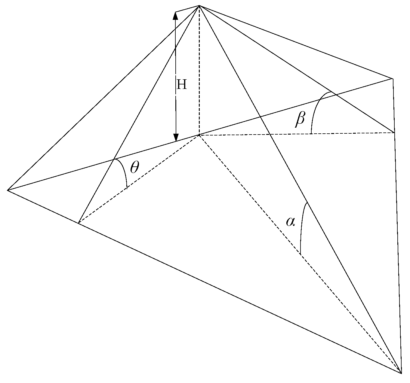
2. Three-Dimensional Model of Natural Ridge Slope

2.1. Establishment of Three-Dimensional Model of Natural Ridge Slope and Wire Frame Model

A considerable part of the natural slope is distributed along the ridge. From the perspective of two-dimensional analysis, it is generally believed that slope stability is closely related to the slope angle, and the safety factor of the slope with a large slope angle is relatively low. However, the structure of the ridge slope is relatively complex, and the complexity and difference in its stress distribution are often ignored when the analysis is simplified to a plane strain problem, which leads to a deviation in the understanding of its overall stability. At the same time, when a slope instability occurs in nature, the sliding surface usually presents a three-dimensional form, but the slope stability analysis still adopts the two-dimensional method. Compared with the three-dimensional analysis method, the two-dimensional analysis method obtains relatively conservative results. In addition, the strength parameters of the rock mass may be overestimated when back analyzing the rock mass strength parameters of the unstable slope. Therefore, it is necessary to establish a three-dimensional model of the ridge slope for research.
A ridge is a convex landform formed by the combination of two opposite slopes with different inclines to form a strip ridge extension. The ridge line is the connection of the highest point of the ridge; that is, the intersection of two slopes. Figure 1 shows a typical ridge slope schematic. The control elements of the ridge slope for simplifying the ridge slope using a wire frame model were determined to be the ridgeline dip angle, two flank slope feet, and the slope height. Figure 2 presents a diagram of an average ridge slope. The angle of the front edge of the mountain ridge and the horizontal plane was α, the right-wing slope angle was β, the left-wing slope feet was θ, and the slope height was H. The model was simplified based on the actual slope. Different ridge slopes can be simulated by adjusting α, β, θ, and H. In this paper, only the case in which β=θ was considered—that is, the ridge slope—was symmetrical. Considering the boundary effect at the bottom of the ridge slope, a base was set at the bottom of the ridge slope, simulating the stratum below the slope. The three-dimensional geometric model of the complete ridge slope used for numerical simulation is shown in Figure 3. On the side boundaries, the displacements perpendicular to the front, back, left, and right sides were set as zero in a horizontal direction and the others were set as free. The displacements and rotation angles were all fixed at zero on the bottom boundary. A free boundary was adopted on the slope surface.
The slope was mainly composed of the ridge slope and the mountain body (Figure 1). The stability of the ridge slope under different conditions was studied in the current study. Therefore, the mountain part was truncated, and the displacement in the X direction was fixed in the truncated part.

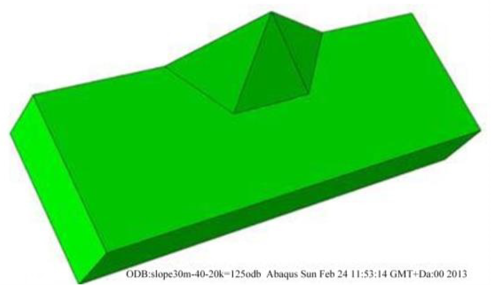
2.2. Geometric Parameters of Natural Ridge Slope Model

The influences of ridgeline dip angle α, flank slope angle β, and slope height H on the stability of the ridge slope were studied. Two factors of the ridge slope were controlled (unchanged), the third factor was changed, and the strength reduction calculation was carried out for comparative analysis. Considering the most common conditions of actual ridge slopes, the value of α ranged from 20° to 60°, the value of β ranged from 30° to 70°, and the values of H were 10, 20, and 30 m. In three-dimensional geometry, αβ must exist; therefore, the combination of αβ in the table cannot make a solid model. The geometric parameters of the ridge slope model are shown in Table 2.

2.3. Physical and Mechanical Parameters of the Ridge and Slope Model

The physical and mechanical parameters were determined and combined with the “Specifications for Water Conservancy and Hydropower Project Slope” and the “Engineering Rock Body Holocating Standards” [36]. Parameters with high strength were selected first according to the principle of strength reduction in finite element calculation. The strength reduction method was used to reduce the shear strength. Then, the plastic zone development process was analyzed when the shear strength of the ridge slope gradually decreased. The physical and mechanical parameters of the slope rock mass were determined according to [37] using empirical analogy, the rock mass quality scoring system, and the connectivity rate method with the judgment results of macroscopic geological conditions. Table 3 shows the physical and mechanical parameters of the ridge slope.

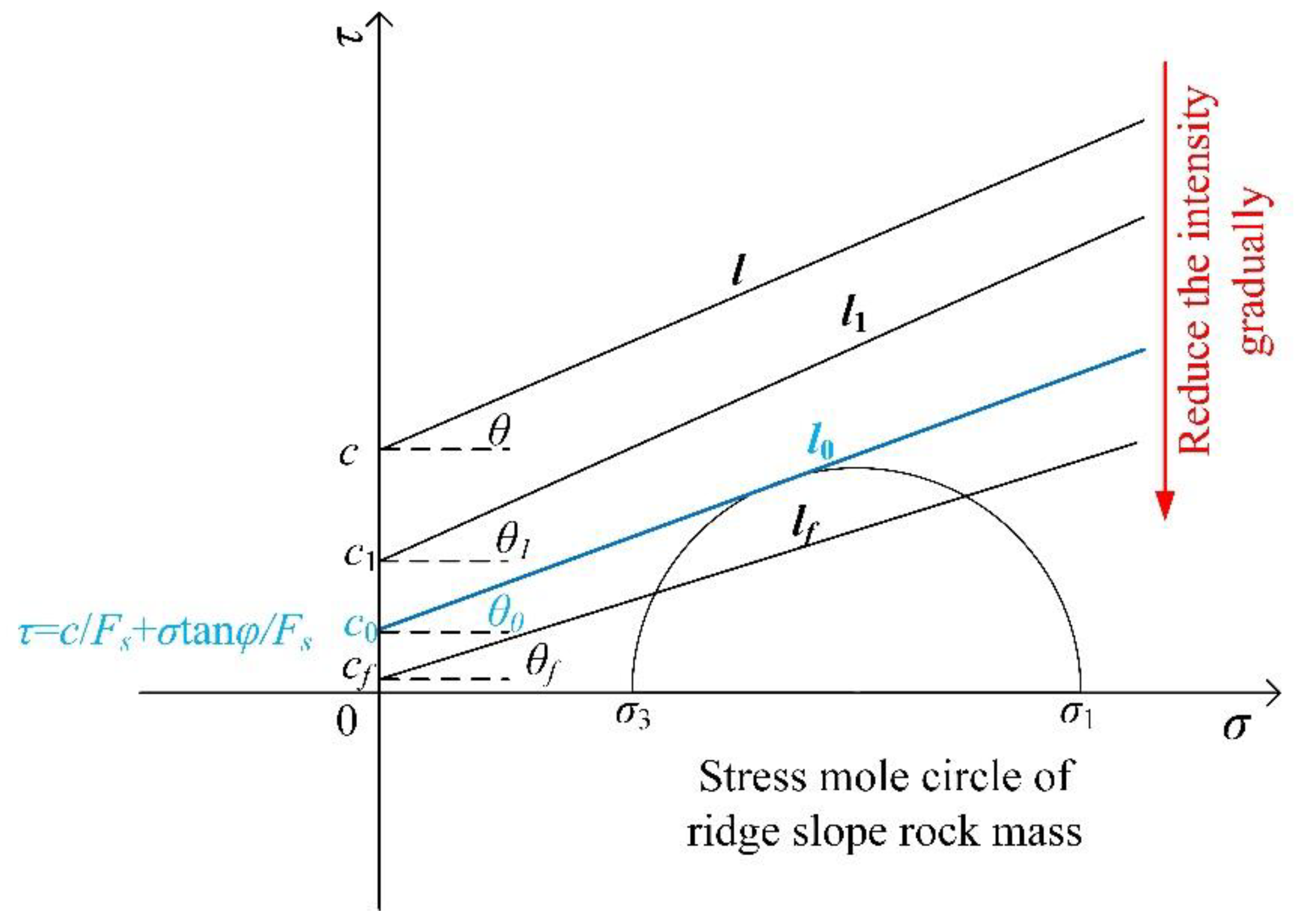
3. Stability Analysis of Ridge Slope

Numerical analysis was performed on the established ridge slope model to study the impact of ridge line inclination α, flank slope angle β, and slope height H on the ridge slope destruction mode. The strength reduction method was used to calculate the displacement and plastic zone of the slope.
Many test results showed that geotechnical materials followed unified intensity theory when the intermediate main stress coefficient (b) was 0.5 [37]. Based on the mechanical model and mathematical expression of the unified strength theory, a corresponding user interface subroutine UMAT (User-defined Material Mechanical Behavior) was written in Fortran language according to the basic elements of elastoplastic constitutive relation proposed in classical elastoplastic mechanics, which was connected to ABAQUS software. The main stress coefficient was 0.5; this was used to calculate the safety factor for the strength reduction method. The software environment used in this study was Windows 8, the hardware environment was Intel(R) Core (TM)2 Duo CPU, NVIDIA GeForce GT240/ATI HD4670, and the RAM was 8 GB. The version of ABAQUS was 6.13.
In this study, the strength reduction method was used to study the stability of the ridge slope. In general, the strength envelope (l) of the ridge slope rock was in a state of separation from the stress circle of the current state, and the ridge slope was in a stable state with relatively small deformation. With the gradual increase in the reduction coefficient, when the strength envelope (l0) was tangent to the Mohr circle of rocks on the ridge slope, the ridge slope was in the limit equilibrium state. With the further increase in the reduction factor, as shown in Figure 4, the strength envelope (lf) intersected the stress circle of the current state. At this time, instability and failure of the ridge and slope had occurred, resulting in a large displacement. Through a strength reduction method, the ridge and slope became unstable. The ridge slope underwent a large displacement.
ABAQUS software was used to simulate the stability of the ridge slope under different conditions. During the calculation process of ABAQUS software, the "Nlgeom" large deformation analysis was initiated in the analysis step. When the strength reduction was not performed or the strength reduction factor was small, the ridge slope was in a relatively stable state in which the displacement of the ridge slope was only a few millimeters. However, the stability of the ridge slope under different conditions cannot be obtained. Therefore, the displacements of ridge slope with a reduction factor of 30 was selected to study the stability of the ridge slope. Wang et al. [38] also adopted ABAQUS software and obtained the displacement of the slope top up to 10.37~11.28 m using a strength reduction method to study the displacement field when the slope instability failure occurred.
In unified strength theory, the failure mode of rock mass can be determined by the following equation:
f = 1 1 + b σ 1 + b 1 + b σ 2 N φ σ 3 + 2 c N φ , σ 2 1 sin φ 2 σ 3 + 1 + sin φ 2 σ 1 f = σ 1 b 1 + b N φ σ 2 1 1 + b N φ σ 3 + 2 c N φ , σ 2 1 sin φ 2 σ 3 + 1 + sin φ 2 σ 1 f t = σ 3 σ t
where b is the failure criterion selection parameter, reflecting the influence of intermediate principal stress on material failure. N φ = 1 + sin φ 1 sin φ , φ is the friction angle of rock material, σt is the tensile strength of a rock material. σ1, σ2, and σ3 are the maximum, intermediate, and minimum principal stresses, respectively. When σ3 is greater than the tensile strength of rock and soil mass, tensile cracking failure occurs; otherwise, shear failure occurs.

3.1. Deformation and Failure Characteristics of Ridge Slope under Different Ridgeline Dip Angles

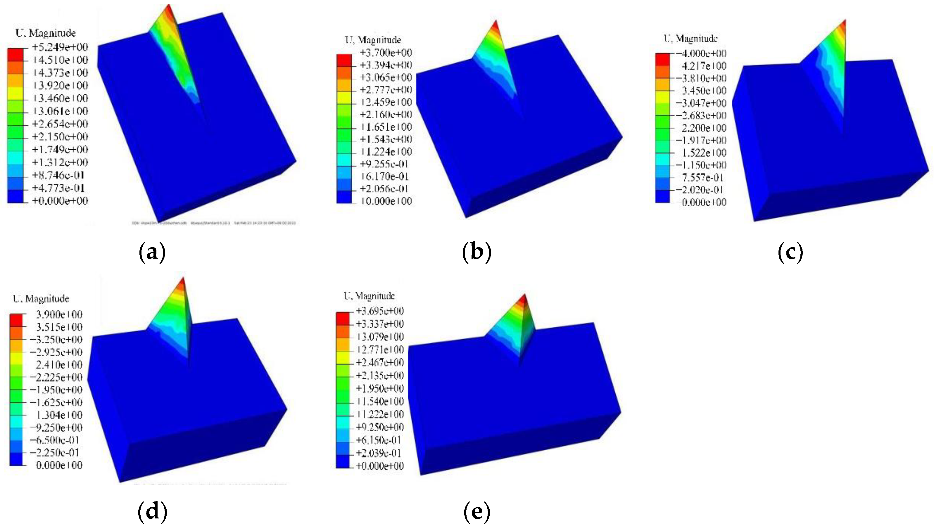
3.1.1. Deformation Characteristics of Ridge Slope under Different Ridgeline Dip Angles

When the flank slope angle (β) of the ridge slope was 70° and the slope height was 10 m, the displacement field and plastic zone of the ridge slope under different ridgeline dip angles α (20°, 30°, 40°, 50°, and 60°) are shown in Figure 5 and Figure 6, respectively. In this study, the displacement was the vector sum of the displacement in the x direction, y direction, and z direction.
The displacement distribution law of the ridge slope was similar when the flank slope angle and the slope height were the same and the ridgeline inclination angle was different (Figure 5). The maximum displacement occurred at the top of the slope at different ridgeline inclination angles; when the ridgeline inclination angle was 20°, the displacement near the top of the slope was at its largest, and the maximum displacement reached 3.8~4.5 m. When the ridgeline inclination angle was 30°, the maximum displacement was 2.7~3.39 m. When the ridgeline inclination angle was 40°, the maximum displacement was 3.45~4.21m. When the ridgeline inclination angle was 50° and 60°, the maximum displacement was 2.77~3.90 m. The displacement of the slope decreased and was distributed in layers as the height decreased.

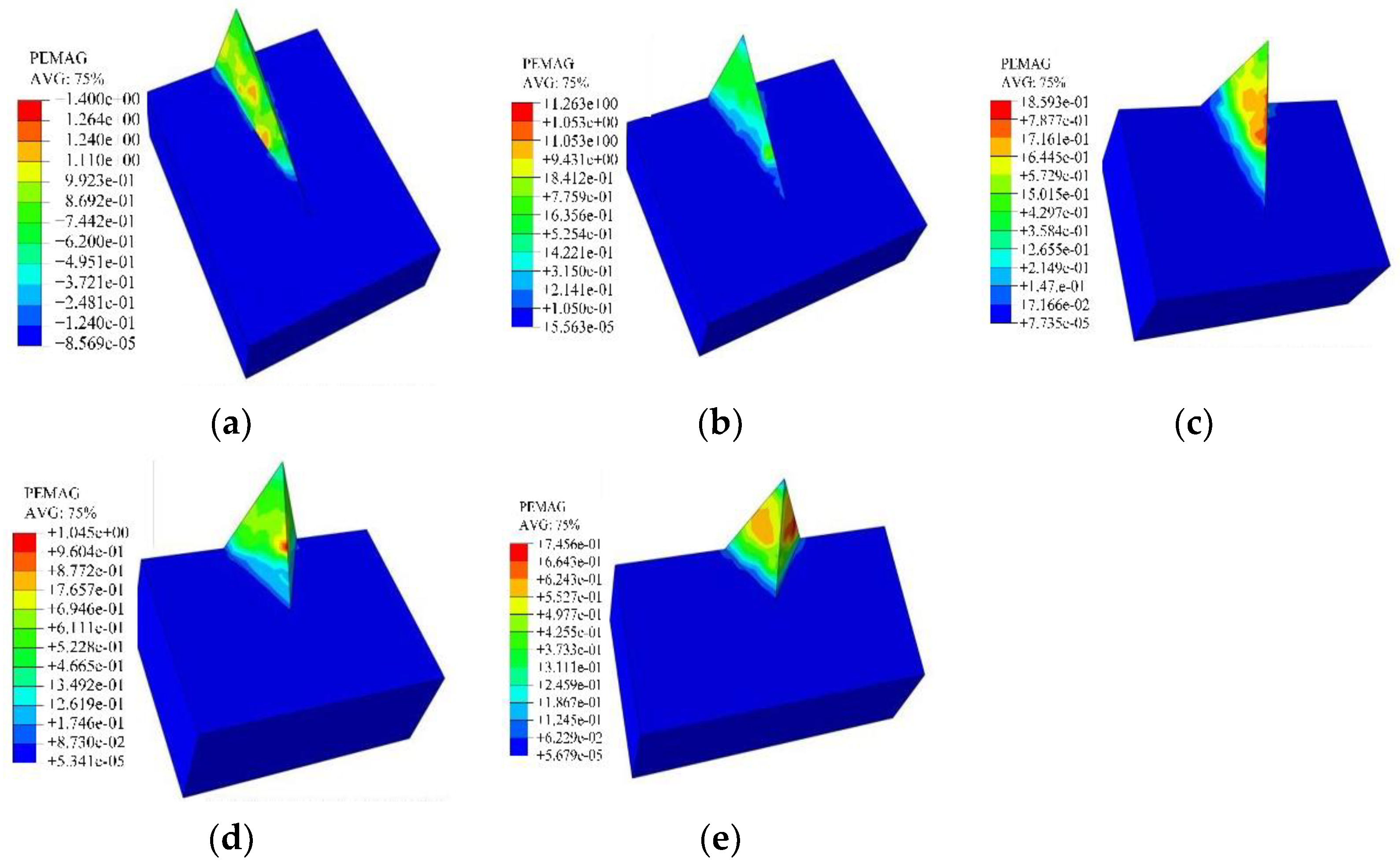
3.1.2. Failure Characteristics of Ridge Slope under Different Ridgeline Dip Angles

Figure 6 shows the cloud map of the plastic zone of the ridge slope under different ridgeline angles (α).
When β and H were unchanged, α = 20°, the largest area of the plastic zone appeared at the front end of the slope of the flank, near the ridgeline (Figure 6). The largest plastic zone gradually moved from the front end of the flank slope to the rear of the slope with the increase in α. When α = 60°, the largest plastic zone was near the rear edge of the slope.
The distribution of plastic deformation of ridge slope could be observed in the plastic zone, and the region with large plastic displacement was prone to failure. When the ridgeline angle of the ridge slope was small, the plastic displacement was mainly distributed in the back edge of the slope (Figure 6), where the failure was prone to occur. When the ridgeline angle of the ridge slope was large, the plastic displacement was mainly distributed near the front of the slope, and the most vulnerable area of the ridge slope was near the front of the slope.

3.1.3. Stability of Ridge Slope under Different Ridgeline Dip Angles

Figure 7 shows the relationship between the displacement at the maximum displacement (at the Apex of the ridge slope) and the reduction coefficient at different ridgeline inclination angles.
Figure 7a shows the relationship between the reduction coefficient and the vertex displacement of the ridge under different α values when β = 70° and H = 10 m. When the reduction coefficient was less than six, no displacement of the ridge slope occurred under different ridgeline angles (Figure 7). When the reduction factor was 8, the ridge slope with α = 20° exhibited a displacement inflection point, indicating that the safety factor of the slope at this time was eight. When the reduction factor gradually increased to 10, the ridge slope at other angles also displayed an inflection point. The smaller the ridgeline inclination angle of the ridge slope, the worse its stability.
When β = 60°, H = 10 m, or β = 50°, H = 10 m, the displacement of the ridge slope did not change with the reduction coefficient, and when the reduction coefficient was greater than six, the displacement of the ridge slope increased uniformly with the reduction coefficient under different ridgeline inclination angles (Figure 7b,c). β also had a great influence on the displacement of the ridge slope (Figure 7). The influence of β on the ridge slope displacement was analyzed.

3.2. Deformation and Failure Characteristics of Ridge Slope under Different Flank Angles

3.2.1. Deformation Characteristics of Ridge Slope under Different Flank Slope Angles

The ridgeline inclination angle of the ridge slope (α) was 20° and the slope height H was 10 m. The displacement cloud of the ridge slope under different mountain wing slopes β (30°, 40°, 50°, 60°, and 70°) is shown in Figure 8.
The maximum displacement of the ridge slope occurred at the top of the slope under the different flank slope angles (Figure 8). When β was small, the area of the large displacement was relatively large, and large displacements occurred in a wide range at the bottom of the ridge slope. When the flank angle was 30°, the maximum displacement of the bottom bedrock was 45.6 cm, which was distributed circularly at the bottom of the mountain slope. However, with the increase in β, the displacement area gradually concentrated on the slope, while the bedrock at the bottom of the ridge slope did not produce a large displacement.

3.2.2. Failure Characteristics of Ridge Slope under Different Flank Slope Angles

Figure 9 shows the plastic zone cloud of the ridge slope under the same ridgeline inclination angle and slope height and different ridgeline inclination angles.
The range of the plastic zone gradually decreased with the increase in β (Figure 9). The stability of the ridge slope was greatly affected by the surrounding strata when β was small, and the slope transmitted part of the force to the surrounding strata. With the increase in β, the force transmitted by the slope to the surrounding strata gradually decreased and became more dependent on the stability of its own rock mass, also reducing the stability of the slope, which was consistent with the actual situation; that is, the steeper the slope, the more unstable it was. The position of the plastic zone was also affected by β; that is, when β was small, the plastic zone was mainly on the slope of the flanks. At this time, the area most prone to damage from the slope was on the flank slope, e.g., sliding along the slope. With the increase in β, the plastic zone concentrated near the ridge line, and the slope became prone to failure along the ridge line.

3.2.3. Stability of Ridge Slope under Different Flank Slope Angles

Figure 10 shows the relationship between the displacement at the maximum displacement (at the apex of the ridge) and the reduction coefficient at different ridgeline inclination angles.
Figure 10a shows that when slope height H and α were the same, the stability of the ridge slope decreased with the increase in β. When β was 70°, the stability coefficient of the ridge slope was seven. When β was 60° and 50°, the displacement curves of the ridge slope in the two cases were basically the same, and the stability coefficient of the slope was 10 at this time. When β was reduced to 40° and 30°, the stability factor of the ridge slope reached 15.
Figure 10b shows the displacement curve of the ridge slope with the reduction coefficient when α = 20°, H = 20 m, and β changes from 30° to 70°. When H and α were the same, the larger the β value, the greater the displacement of the slope under the same reduction coefficient (Figure 10b). Compared with the case of H = 10 m in Figure 10a, when the slope height was high, the displacement of the slope increased obviously with the increase in β. The greater the slope height, the more prominent the influence of β on the stability of the slope.

3.3. Deformation and Failure Characteristics of Ridge Slopes with Different Slope Heights

3.3.1. Deformation Characteristics of Ridge Slope under Different Slope Heights

This section maintained ridge-line inclination α and flank slope angle β, resulting in the change in the slope height between 10 and 30 m, and the stress field and plastic zone variation law of the ridgeline slope were studied. Figure 11 shows the displacement cloud map of the ridge slope under different slope heights (10, 20, and 30 m) with the ridge-line inclination of 20° and the flank slope angle of 30°.
The displacement distribution laws in the ridge slope displacement cloud map were similar under different slope heights (Figure 11). The maximum displacement occurred at the top of the slope, and the higher the slope height, the greater the displacement at the top of the slope. When the slope height was 10 m, the displacement at the top of the slope was 1.5 m. When the slope height increased to 30 m, the displacement at the top of the slope reached as high as 14.7 m. The displacement was the same in the underslope part of the ridge slope. The bedrock at the bottom of the ridge slope had a large displacement, and the higher the slope height was, the larger the displacement and the displacement area were.

3.3.2. Failure Characteristics of Ridge Slope under Different Slope Heights

Figure 12 shows the plastic zone of the ridge slope under the same ridgeline inclination angle, flank slope angle, and different slope heights.
Figure 12 shows that the larger the height of the ridge slope, the larger its plastic area, and the plastic strain was also increasing. When the height was small, the plastic zone mainly occurred at the back edge of the slope, easily cracking the back edge. When the height of the ridge slope increased, a large plastic zone appeared at the front of the slope, and the bottom of the flank slope was also displaced. When the slope of the ridge increased slowly, the maximum plastic strain of the slope occurred at the top of the slope compared with those in Figure 11 and Figure 12. When the slope increased, the plasticity zone began to appear at the foot of the slope, indicating that it was prone to squeeze and damage.

3.3.3. Stability of Ridge Slope under different Slope Heights

The relationship between the displacement at the top of the ridge slope and the reduction coefficient was presented to study the influence of slope height on the stability of ridge slope more intuitively (Figure 13).
The slope height had a great impact on the stability of the ridge slope when α and β were the same (Figure 13). When the reduction coefficient was the same, the higher the slope height, the greater the displacement of the slope body. When the slope height was 30 m and the reduction coefficient was greater than four, the displacement of the ridge slope increased significantly with the increase in the reduction coefficient. The slope was in a critical failure state at this time, indicating that the safety and stability coefficient of the slope body at this time was four. When the slope height was 10 m, the displacement curve grew slowly, indicating that the slope nearly remained stable when the slope height was 10 m.

4. Numerical Simulation Study on Stability of Ridge and Slope after Excavation

4.1. Simulation of Excavation Model

The variation law of the displacement field and the plastic zone of the ridge slope after excavation under different excavation slope rates (1:1, 1:1.25, and 1:1.5) was studied to observe the influence degree of the excavation slope rate on the stability of the ridge slope. Figure 14a shows a schematic of ridge slope excavation. If a highway passes through the area, then slope excavation is required. The slope in the red line represents the part to be excavated. As shown in Figure 14b, point B was the midpoint of the intersection between the ridge slope and the road. OA was the height of point O, and the slope rate of the excavation was i = OA/AB = h/l.

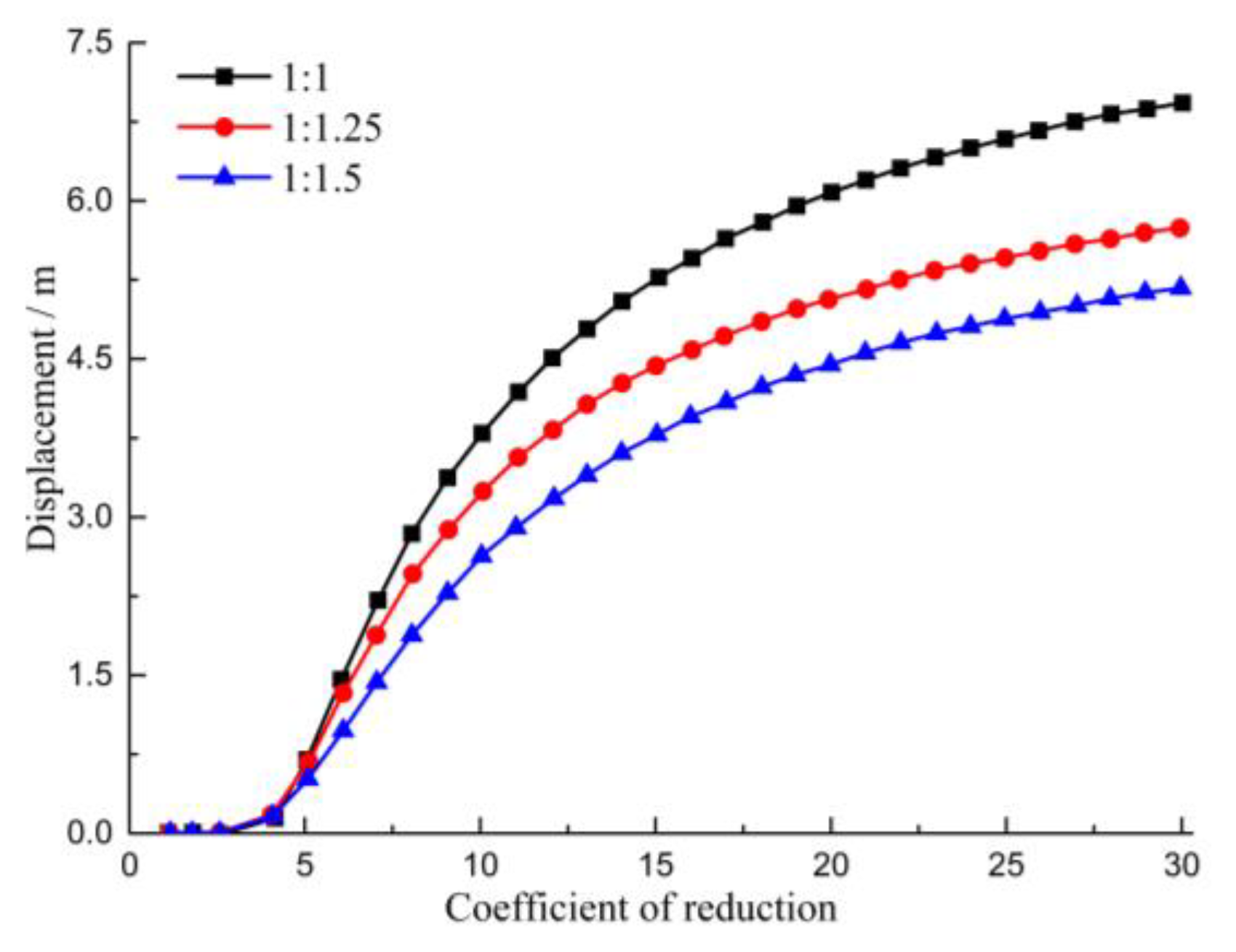
4.2. Stability of Ridge Slope under Different Excavation Slope Ratio

In actual engineering, if the slope height is small, then it can be directly excavated without considering the influence of excavation. The effect of the excavation slope rate was considered only when the slope height was large, so the slope height was set to 30 m in this paper. Figure 15 presents the displacement cloud map of the ridge slope under different excavation slope ratios when α is 20° and β is 40°.
The maximum displacement occurred at the top of the slope under different excavation slope rates, and the greater the excavation slope rate, the greater the displacement at the top of the slope (Figure 15). The displacement of the flank slope also increased with the excavation slope ratio. When the excavation slope ratio was small, the displacement of the lower part of the ridge slope and the disturbance of the excavation effect on the bedrock at the bottom of the slope were small. However, when the excavation slope rate was large, the bedrock at the bottom of the slope displayed a large displacement, and the area of the bedrock deformation zone was also large.
Figure 16 shows the cloud map of the plastic zone of the ridge slope under different excavation slope rates when α is 20° and β is 40°.
The larger the excavation slope ratio, the larger the plastic zone area and plastic displacement of the ridge slope. When the excavation slope ratio was 1:1.5, the plastic strain of the ridge slope was 2.89, and very little plastic displacement occurred on the excavation surface. When the excavation slope ratio increased to 1:1, the plastic displacement of the excavation slope increased, and even a penetrated plastic zone appeared. A plastic zone also existed in the area of the slope toe. Therefore, appropriate reinforcement treatment was required at the slope foot.
Figure 17 shows the relationship between the displacement at the top of the slope and the strength reduction coefficient under different excavation slope rates.
The curves of the displacement at the top of the slope with the reduction coefficient at different excavation slope rates. The safety factor of the excavated slope was indeed reduced compared with the original slope. The comparison of the displacement curves of three different excavation slope ratios indicates that the stability coefficient of the slope with a small slope rate was small. When the excavation slope rate was small, the excavation volume was large, and the slope extended to the back of the ridge side slope. The slope surface was greatly affected by the displacement of the trailing edge of the slope, so the stability coefficient of the ridge slope was low at this time (Figure 17).
In the calculation of H = 30 m, α = 30°, and β = 40°, even when the excavation slope rate was 1:1, the excavated slope still reached the peak of the ridge when excavating the ridge slope. Therefore, the slope was cut from the top of the ridge slope, and the slope ratio was 1:0.9, which satisfied the road width requirement. The slope after cutting is shown in Figure 18, and the displacement cloud and plastic zone maps are shown in Figure 19.
When the excavation slope ratio was 1:0.9, the displacement at the top of the ridge slope was the largest, and a large displacement also occurred on the excavation slope surface at this time (Figure 19b). As shown in Figure 19b, when the excavation slope ratio increased to 1:0.9, the plastic zone of the slope was transferred from the position of the flank slope to the area of the slope. That is, the closer the cutting position was to the trailing edge of the ridge slope, the larger the plastic zone of the cutting slope surface was, and the more prone it was to instability.

5. Conclusions

In this paper, a geometric model of a ridge slope was constructed, based on the unified strength theory, and the stability of a ridge slope under different working conditions was studied by using strength reduction method. The following conclusions were reached.
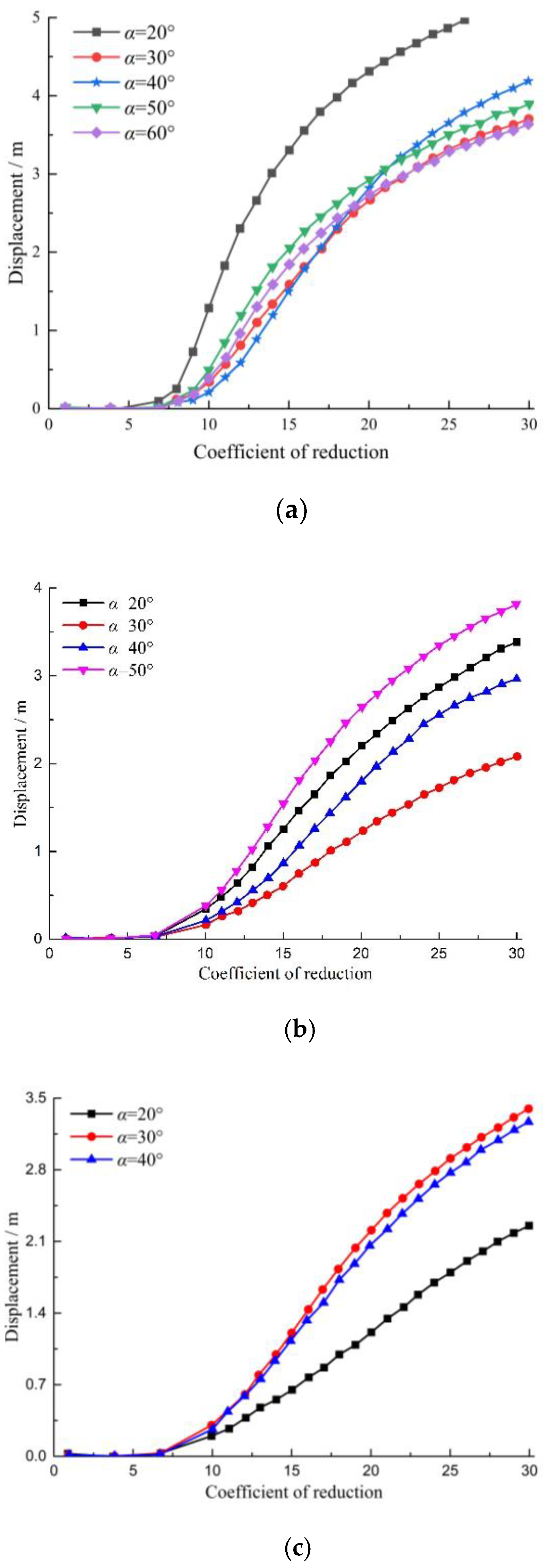
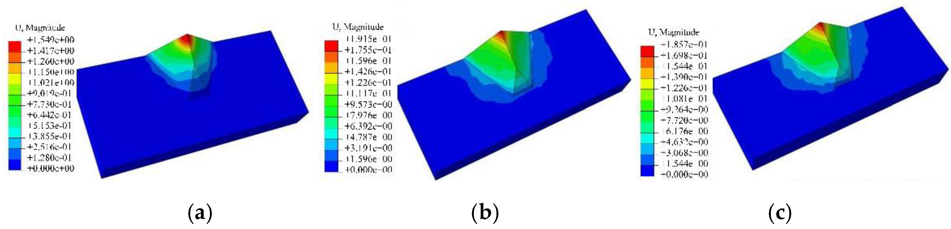
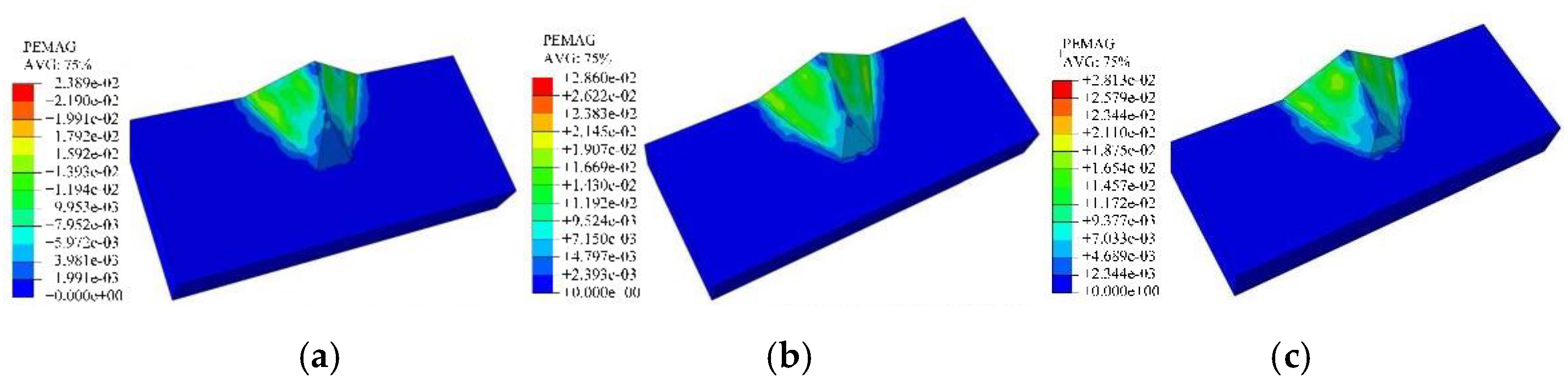
  • No displacement of the ridge slope occurred under different α values when the reduction factor was less than six. The smaller the α of the ridge slope, the worse its stability. When α = 20°, the stability coefficient of the ridge slope was 8, and when α was greater than 20°, the stability coefficient of the ridge slope increased to 10.
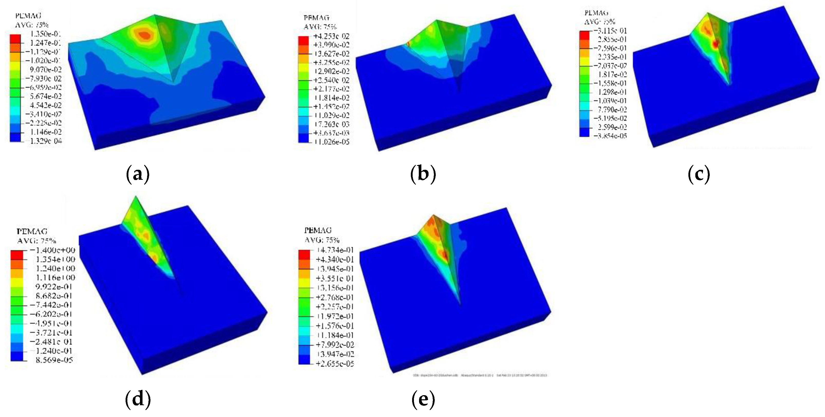
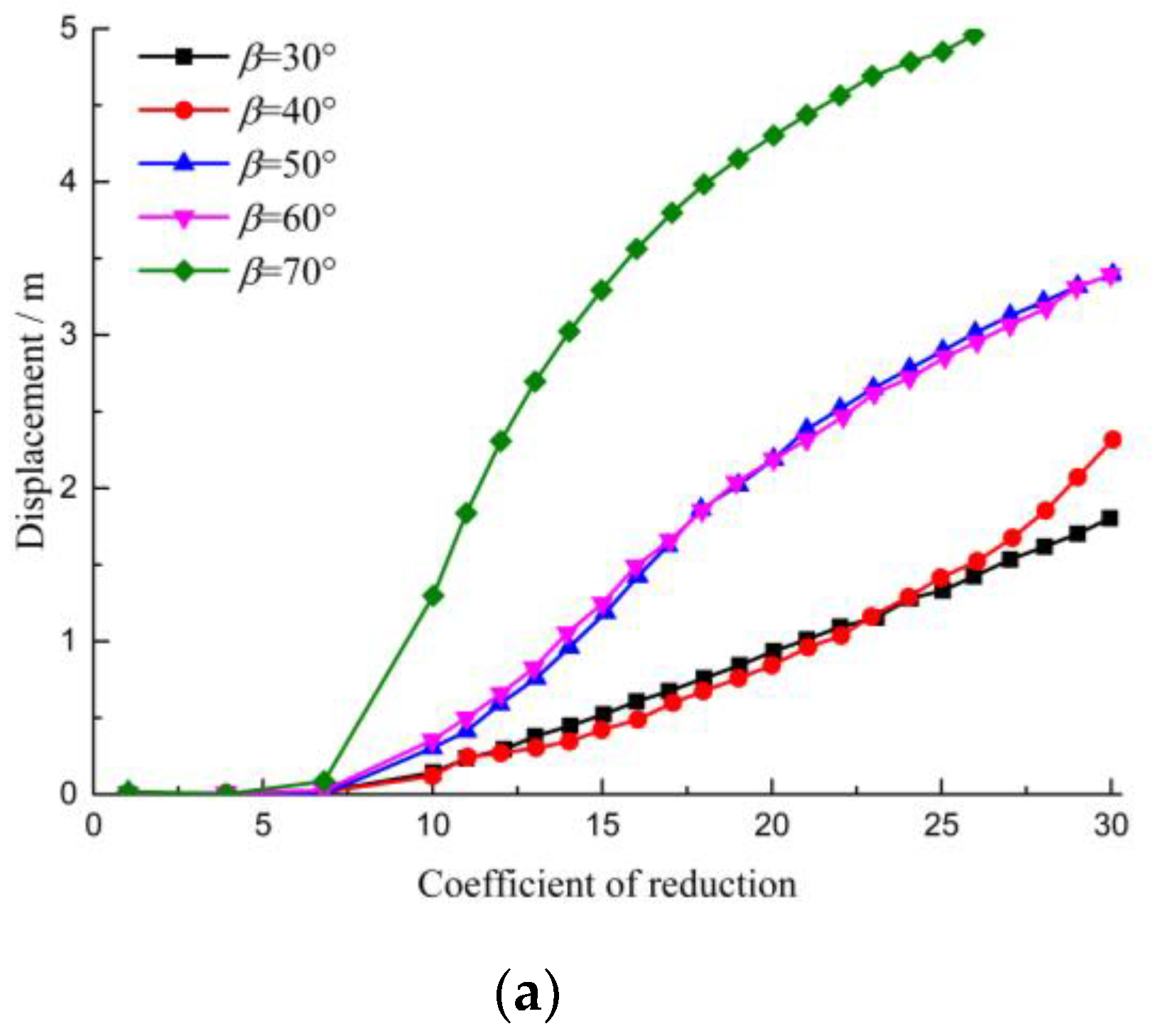
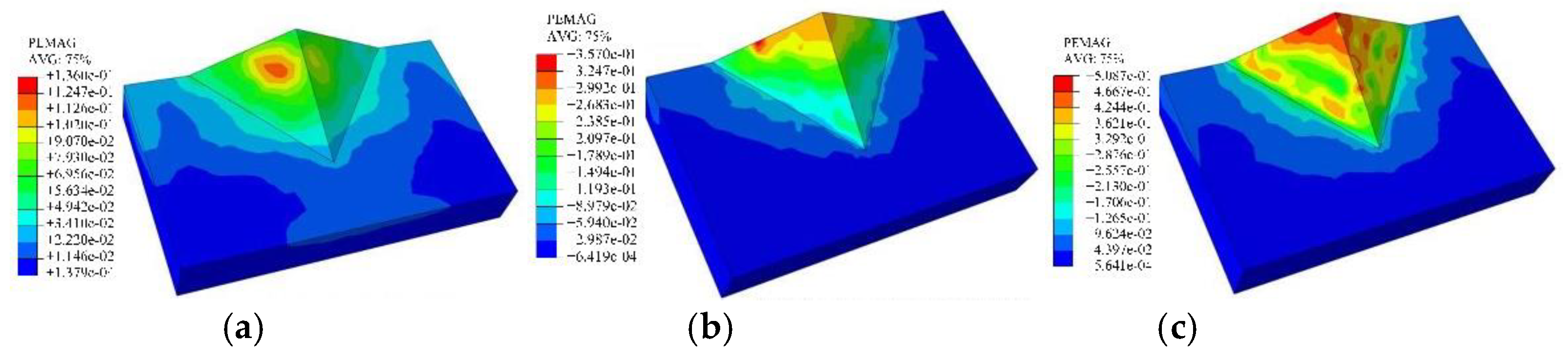
  • When the β was small, the plastic area was distributed in a flank slope position, and the plastic area gradually concentrated to the ridge as β increased. When the β was 70 °, the stabilization coefficient of the ridge slope was 7. When the β decreased to 40° and 30°, the stability coefficient of the ridge slope reached 15. Under the same reduction factor, the larger the β of the ridge slope, the larger the displacement, and the ridge slope was more prone to instability.
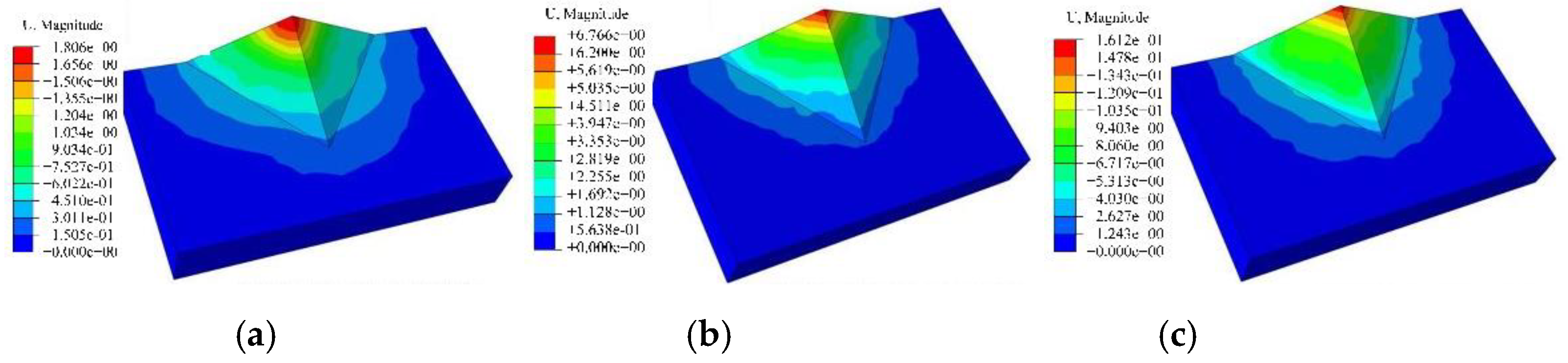
  • The higher the slope height was, the larger the displacement at the top of the slope was. The reduction coefficient of the ridge slope curve increased gently, and the instability phenomenon of the slope hardly occurred. When the slope height increased to 30 m, the displacement at the top of the slope was 14.7 m, and the safety and stability coefficient of the slope was 4.
  • When the excavation slope rate was large, the bedrock exhibited a large displacement; the plastic zone and a large displacement began to appear on the excavation slope surface because of the close proximity of the excavation surface position to the back edge of the ridge slope. Therefore, the ridge slope is more prone to instability.

Author Contributions

Conceptualization, J.W.; Methodology, J.W., P.S. and F.W.; Software, J.W. and P.S.; Validation, J.W., P.L., P.S., H.L., F.W., Y.S. (Yuxin Su), Y.L., A.C., Y.S. (Yuanwei Sun) and Q.Z.; Formal analysis, J.W. and P.S.; Investigation, J.W., P.S., H.L., F.W., Y.S. (Yuxin Su), Y.L., A.C., Y.S. (Yuanwei Sun) and Q.Z.; Data curation, J.W., P.S., H.L., F.W., Y.S. (Yuxin Su), Y.L., A.C., Y.S. (Yuanwei Sun) and Q.Z.; Writing—original draft, J.W., P.L. and P.S.; Writing—review & editing, J.W. and P.L.; Supervision, J.W.; Funding acquisition, J.W. All authors have read and agreed to the published version of the manuscript.

Funding

This research was funded by the Shanghai Municipal Science and Technology Project (18DZ1201300;19DZ1200900); the Xiamen Road and Bridge Group (XM2017-TZ0151; XM2017-TZ0117); the project of the Key Laboratory of Impact and Safety Engineering (Ningbo University), Ministry of Education (CJ202101); the Shanghai Municipal Science and Technology Major Project (2021SHZDZX0100) and the Fundamental Research Funds for the Central Universities; the Key Laboratory of Land Subsidence Monitoring and Prevention, Ministry of Natural Resources of China (No. KLLSMP202101; KLLSMP202201); Suzhou Rail Transit Line 1 Co. Ltd., and China Railway 15 Bureau Group Co. Ltd.

Institutional Review Board Statement

Not applicable.

Informed Consent Statement

Not applicable.

Data Availability Statement

Not applicable.

Conflicts of Interest

The authors declare no conflict of interest.

References

  1. Liu, Y.; Li, X.; Liu, X.; Yang, Z. A combined shear strength reduction and surrogate model method for efficient reliability analysis of slopes. Comput. Geotech. 2022, 152, 105021. [Google Scholar] [CrossRef]
  2. Chen, X.; Ren, J.; Wang, D.; Lyu, Y.; Zhang, H. A Generalized Strength Reduction Concept and Its Applications to Geotechnical Stability Analysis. Geotech. Geol. Eng. 2019, 37, 2409–2424. [Google Scholar] [CrossRef]
  3. Xu, Q.; Yin, H.; Cao, X.; Li, Z. A temperature-driven strength reduction method for slope stability analysis. Mech. Res. Commun. 2009, 36, 224–231. [Google Scholar] [CrossRef]
  4. Li, P.F.; Liu, H.B.; Zhang, Y. Based on The Strength Reduction Slope Stability Finite Element Analysis of Engineering Examples: Progress in Civil Engineering, PTS 1–4[Z]. In Proceedings of the 2nd International Conference on Civil Engineering, Architecture and Building Materials (CEABM 2012), Yantai, China, 25–27 May 2012; Volume 170–173, pp. 885–888. [Google Scholar]
  5. Illeditsch, M.; Preh, A.; Sausgruber, J.T. Challenges Assessing Rock Slope Stability Using the Strength Reduction Method with the Hoek-Brown Criterion on the Example of Vals (Tyrol/Austria). Geosciences 2022, 12, 255. [Google Scholar] [CrossRef]
  6. Chen, Q.; Bai, B.; Wang, H.; Li, X. Dissipated Energy as the Evaluation Index for the Double Reduction Method. Int. J. Geomech. 2021, 21, 6021012. [Google Scholar] [CrossRef]
  7. Yang, Y.; Xia, Y.; Zheng, H.; Liu, Z. Investigation of rock slope stability using a 3D nonlinear strength-reduction numerical manifold method. Eng. Geol. 2021, 292, 106285. [Google Scholar] [CrossRef]
  8. An, X.; Li, N. Non-Equal Strength Reduction Analysis of Soil Slopes Considering Progressive Failure. Soil Mech. Found. Eng. 2021, 58, 273–279. [Google Scholar] [CrossRef]
  9. Hu, L.; Takahashi, A.; Kasama, K. Effect of spatial variability on stability and failure mechanisms of 3D slope using random limit equilibrium method. Soils Found. 2022, 62, 101225. [Google Scholar] [CrossRef]
  10. Li, S.; Zhao, Z.; Hu, B.; Yin, T.; Chen, G.; Chen, G. Hazard Classification and Stability Analysis of High and Steep Slopes from Underground to Open-Pit Mining. Int. J. Environ. Res. Public Health 2022, 19, 11679. [Google Scholar] [CrossRef]
  11. Ding, Q.L.; Peng, Y.Y.; Cheng, Z.; Wang, P. Numerical Simulation of Slope Stability during Underground Excavation Using the Lagrange Element Strength Reduction Method. Minerals 2022, 12, 1054. [Google Scholar] [CrossRef]
  12. Li, Y.; Qian, C.; Fu, Z.; Li, Z. On Two Approaches to Slope Stability Reliability Assessments Using the Random Finite Element Method. Appl. Sci. 2019, 9, 4421. [Google Scholar] [CrossRef] [Green Version]
  13. Dyson, A.P.; Tolooiyan, A. Optimisation of strength reduction finite element method codes for slope stability analysis. Innov. Infrastruct. Solut. 2018, 3, 38. [Google Scholar] [CrossRef]
  14. Luan, M.; Wu, Y.; Nian, T. An Alternative Criterion for Evaluating Slope Stability Based on Development of Plastic Zone by Shear Strength Reduction FEM. J. Disaster Prev. Mitig. Eng. 2003, 23, 1–8. [Google Scholar]
  15. Shi, B.T.; Zhang, Y.; Zhang, W. Strength reduction material point method for slope stability. Chin. J. Geotech. Eng. 2016, 38, 1678–1684. [Google Scholar]
  16. Ahangari Nanehkaran, Y.; Pusatli, T.; Chengyong, J.; Chen, J.; Cemiloglu, A.; Azarafza, M.; Derakhshani, R. Application of Machine Learning Techniques for the Estimation of the Safety Factor in Slope Stability Analysis. Water 2022, 14, 3743. [Google Scholar] [CrossRef]
  17. Nanehkaran, Y.A.; Licai, Z.; Chen, J.; Azarafza, M.; Yimin, M. Application of artificial neural networks and geographic information system to provide hazard susceptibility maps for rockfall failures. Environ. Earth Sci. 2022, 81, 475. [Google Scholar] [CrossRef]
  18. Azarafza, M.; Nanehkaran, Y.A.; Rajabion, L.; Akgün, H.; Rahnamarad, J.; Derakhshani, R.; Raoof, A. Application of the modified Q-slope classification system for sedimentary rock slope stability assessment in Iran. Eng. Geol. 2020, 264. [Google Scholar] [CrossRef]
  19. Bai, B.; Yuan, W.; Li, X. A new double reduction method for slope stability analysis. J. Cent. South Univ. 2014, 21, 1158–1164. [Google Scholar] [CrossRef]
  20. Wang, H.; Yang, Y.; Sun, G.; Zheng, H. A stability analysis of rock slopes using a nonlinear strength reduction numerical manifold method. Comput. Geotech. 2021, 129, 103864. [Google Scholar] [CrossRef]
  21. Wang, H.; Zhang, B.; Mei, G.; Xu, N. A statistics-based discrete element modeling method coupled with the strength reduction method for the stability analysis of jointed rock slopes. Eng. Geol. 2020, 264, 105247. [Google Scholar] [CrossRef]
  22. Deng, D.; Li, L.; Zhao, L. Limit equilibrium method (LEM) of slope stability and calculation of comprehensive factor of safety with double strength-reduction technique. J. Mt. Sci. 2017, 14, 2311–2324. [Google Scholar] [CrossRef]
  23. Yuan, W.; Bai, B.; Li, X.C.; Wang, H.B. A strength reduction method based on double reduction parameters and its application. J. Cent. South Univ. 2013, 20, 2555–2562. [Google Scholar] [CrossRef]
  24. Wei, Y.; Jiaxin, L.; Zonghong, L.; Wei, W.; Xiaoyun, S. A strength reduction method based on the Generalized Hoek-Brown (GHB) criterion for rock slope stability analysis. Comput. Geotech. 2020, 117, 103240. [Google Scholar] [CrossRef]
  25. Chen, Z.; Lei, J.; Huang, J. Finite element limit analysis of slope stability considering spatial variability of soil strengths. Chin. J. Geotech. Eng. 2018, 40, 985–993. [Google Scholar]
  26. Xu, Z.; Li, C.; Fang, F.; Wu, F. Study on the Stability of Soil-Rock Mixture Slopes Based on the Material Point Strength Reduction Method. Appl. Sci. 2022, 12, 11595. [Google Scholar] [CrossRef]
  27. Yang, Y.; Chen, T.; Wu, W.; Zheng, H. Modelling the stability of a soil-rock-mixture slope based on the digital image technology and strength reduction numerical manifold method. Eng. Anal. Bound. Elem. 2021, 126, 45–54. [Google Scholar] [CrossRef]
  28. Zhang, W.L.; Sun, X.Y.; Chen, Y. Slope stability analysis method based on compressive strength reduction of rock mass. Rock Soil Mech. 2022, 43, 607–615. [Google Scholar]
  29. Lin, H.; Wang, W.; Li, A. Investigation of dilatancy angle effects on slope stability using the 3D finite element method strength reduction technique. Comput. Geotech. 2020, 118, 103295. [Google Scholar] [CrossRef]
  30. Cheng, Y.M.; Lansivaara, T.; Wei, W.B. Reply to “Comments on ‘Two-dimensional slope stability analysis by limit equilibrium and strength reduction methods’ by Y.M. Cheng, T. Lansivaara and W.B. Wei,” by J. Bojorque, G. De Roeck and J. Maertens. Comput. Geotech. 2008, 35, 309–311. [Google Scholar] [CrossRef]
  31. Nie, Z.; Zhang, Z.; Zheng, H. Slope stability analysis using convergent strength reduction method. Eng. Anal. Bound. Elem. 2019, 108, 402–410. [Google Scholar] [CrossRef]
  32. Sarkar, S.; Chakraborty, M. Stability analysis for two-layered slopes by using the strength reduction method. Int. J. Geo-Eng. 2021, 12, 24. [Google Scholar] [CrossRef]
  33. Wei, W.B.; Cheng, Y.M. Stability Analysis of Slope with Water Flow by Strength Reduction Method. Soils Found. 2010, 50, 83–92. [Google Scholar] [CrossRef] [Green Version]
  34. Qiao, S.F.; Wang, C. Study on safety factor calculation and stability evaluation of dynamic slope based on strength reduction method. Fresenius Environ. Bull. 2019, 28, 5301–5311. [Google Scholar]
  35. Sun, G.; Lin, S.; Zheng, H.; Tan, Y.; Sui, T. The virtual element method strength reduction technique for the stability analysis of stony soil slopes. Comput. Geotech. 2020, 119, 103349. [Google Scholar] [CrossRef]
  36. Ding, Z.J.; Zheng, J.; Lu, Q.; Deng, J.; Tong, M. Discussion on calculation methods of quality index of slope engineering rock mass in Standard for engineering classification of rock mass. Rock Soil Mech. 2019, 40, 275–280. [Google Scholar]
  37. Wu, X.; Jia, Z.X.; Chen, Z.Y.; Wang, X.G.; Yang, J. Research of a synthetical method GMEM on ascertaining shear strength for engineering rock mass. Chin. J. Rock Mech. Eng. 2005, 24, 246–251. [Google Scholar]
  38. Wang, J.Q. Study on Slope Stability Analysis Based on Double Strength Reduction Method. Master’s Thesis, Chongqing University, Chongqing, China, 2019. [Google Scholar]
Figure 1. Diagram of a ridge slope.
Applsci 13 01580 g001
Figure 2. Three -dimensional model of the ridge slope.
Applsci 13 01580 g002
Figure 3. Three-dimensional geometric model of the ridge slope.
Applsci 13 01580 g003
Figure 4. Principle of strength reduction method.
Applsci 13 01580 g004
Figure 5. Displacement cloud map of ridge slope under different ridgeline dip angles (unit: m); (a) α = 20°; (b) α = 30°; (c) α = 40°; (d) α = 50°; (e) α = 60°.
Applsci 13 01580 g005
Figure 6. Cloud map of the plastic zone of ridge slope under different ridgeline inclination; (a) α = 20°; (b) α = 30°; (c) α = 40°; (d) α = 50°; (e) α = 60°.
Applsci 13 01580 g006
Figure 7. Variation curve of displacement at the apex of ridge slope with reduction factor under different α; (a) H = 10 m, β = 70°; (b) H = 10 m, β = 60°; (c) H = 10 m, β = 50°.
Applsci 13 01580 g007
Figure 8. Ridge slope displacement cloud under different flank inclination angles (unit: m); (a) β = 30°; (b) β = 40°; (c) β = 50°; (d) β = 60°; (e) β = 70°.
Applsci 13 01580 g008
Figure 9. Plastic zone cloud map of ridge slope under different flank dip angles; (a) β = 30°; (b) β = 40°; (c) β = 50°; (d) β = 60°; (e) β = 70°.
Applsci 13 01580 g009
Figure 10. Variation curve of ridge apex displacement with reduction coefficient under different β; (a) α = 20°, H = 10 m; (b) α = 20°, H = 20 m.
Applsci 13 01580 g010aApplsci 13 01580 g010b
Figure 11. Displacement cloud map of ridge slop under different slope high (Unit: m) (a) H = 10 m; (b) H = 20 m; (c) H = 30 m.
Applsci 13 01580 g011
Figure 12. The plastic zone cloud map of ridge slope under different slope heights; (a) H = 10 m; (b) H = 20 m; (c) H = 30 m.
Applsci 13 01580 g012
Figure 13. Variation curve of ridge vertex displacement with reduction coefficient under different H.
Applsci 13 01580 g013
Figure 14. Schematic diagram of ridge slope excavation model, (a) pre-excavation; (b) post-excavation.
Applsci 13 01580 g014
Figure 15. The displacement clouds map of ridge slope after excavation under different excavation slope rates (Unit: m). (a) The excavation slope ratio is 1:1.5; (b) the excavation slope ratio is 1:1.25; (c) the excavation slope ratio is 1:1.
Applsci 13 01580 g015
Figure 16. The plastic zone cloud map of ridge slope after excavation under different excavation slope rates. (a) The excavation slope ratio is 1:1.5; (b) the excavation slope ratio is 1:1.25; (c) the excavation slope ratio is 1:1.
Applsci 13 01580 g016
Figure 17. Displacement curves at the top of the slope with different excavation slope ratios.
Applsci 13 01580 g017
Figure 18. Model diagram of the ridge slope after slope cutting (H = 30 m, α = 30°, β = 40°).
Applsci 13 01580 g018
Figure 19. The displacement cloud map and plastic zone cloud map of ridge slope after excavation. (a) Displacement cloud map; (b) plastic zone cloud map.
Applsci 13 01580 g019
Table 1. Method for analysis of slope stability.
MethodAdvantageDisadvantage
Limit equilibrium methodThe physical meaning of parameters and structures is very clear; the formula is simple and easy to understand intuitively.Without considering the relationship between material stress and material strain, the obtained safety factor is only the average safety degree on the assumed sliding surface.
Probability analysis methodThe reliability analysis method can objectively and quantitatively reflect the safety of a slope to a certain extent.The probability model of each factor and its numerical characteristics cannot be reasonably selected, and the calculation process is relatively complex.
Fuzzy mathematical methodIt is convenient to obtain objective and fair evaluation conclusions with strong uncertain information processing ability.There is strong subjectivity when determining attribute weight. The problem of information overlap between evaluation reference levels cannot be solved. The calculation process is complicated.
Neural network methodIt has obvious advantages in solving nonlinear problems and excellent performance in modeling nonlinear multivariate problems.It shows excessive reliance on a large number of data samples, and the computer performance requirements are relatively high, which can easily lead to precision damage.
Grey analysis theoryThe calculated workload is relatively small. Samples do not need to be distributed regularly.The mechanism of connotative mechanics is unclear and there is no clear quantitative description.
Normal finite element reduction methodThe stability factor can be calculated. The instability mechanism can be analyzed.The calculation is time consuming and expensive. Failure mode has been determined before calculation.
Finite element reduction method of unified strength criterionThe stability factor can be calculated. The instability mechanism can be analyzed. Failure mode can be determined through calculation.The calculation is time consuming and expensive.
Table 2. Geometric parameters of the ridge slope model.
H (m) α (°)2030405060
β (°)
103010-30-20----
4010-40-2010-40-30---
5010-50-2010-50-3010-50-40--
6010-60-2010-60-3010-60-4010-60-50-
7010-70-2010-70-3010-70-4010-70-5010-70-60
203020-30-20----
4020-40-2020-40-30---
5020-50-2020-50-3020-50-40--
6020-60-2020-60-3020-60-4020-60-50-
7020-70-2020-70-3020-70-4020-70-5020-70-60
303030-30-20----
4030-40-2030-40-30---
5030-50-2030-50-3030-50-40--
6030-60-2030-60-3030-60-4030-60-50-
7030-70-2030-70-3030-70-4030-70-5030-70-60
Table 3. Physical and mechanical parameters of ridge slope rock mass.
Parameterc (kPa)φ (°)νE (GPa)γ (kN/m3)
Numerical140050.20.355.022.5
Disclaimer/Publisher’s Note: The statements, opinions and data contained in all publications are solely those of the individual author(s) and contributor(s) and not of MDPI and/or the editor(s). MDPI and/or the editor(s) disclaim responsibility for any injury to people or property resulting from any ideas, methods, instructions or products referred to in the content.

