

Timed-SAS: Modeling and Analyzing the Time Behaviors of Self-Adaptive Software under Uncertainty

1
College of Defense Engineering, Rocket Force University of Engineering, Xi’an 710025, China
2
College of Defense Engineering, Army Engineering University of PLA, Nanjing 210007, China
*
Author to whom correspondence should be addressed.
Appl. Sci. 2023, 13(3), 2018; https://doi.org/10.3390/app13032018
Submission received: 21 November 2022
/
Revised: 29 January 2023
/
Accepted: 30 January 2023
/
Published: 3 February 2023
(This article belongs to the Topic Software Engineering and Applications)
Abstract
:Featured Application
The Timed-SAS approach can be used to design and quantitatively analyze the complex self-adaptive software systems, such as cloud computing systems.
Abstract
Self-adaptive software (SAS) is gaining in popularity as it can handle dynamic changes in the operational context or in itself. Time behaviors are of vital importance for SAS systems, as the self-adaptation loops bring in additional overhead time. However, early modeling and quantitative analysis of time behaviors for the SAS systems is challenging, especially under uncertainty environments. To tackle this problem, this paper proposed an approach called Timed-SAS to define, describe, analyze, and optimize the time behaviors within the SAS systems. Concretely, Timed-SAS: (1) provides a systematic definition on the deterministic time constraints, the uncertainty delay time constraints, and the time-based evaluation metrics for the SAS systems; (2) creates a set of formal modeling templates for the self-adaptation processes, the time behaviors and the uncertainty environment to consolidate design knowledge for reuse; and (3) provides a set of statistical model checking-based quantitative analysis templates to analyze and verify the self-adaptation properties and the time properties under uncertainty. To validate its effectiveness, we presented an example application and a subject-based experiment. The results demonstrated that the Timed-SAS approach can effectively reduce modeling and verification difficulties of the time behaviors, and can help to optimize the self-adaptation logic.
1. Introduction
Nowadays, complex software systems such as the cloud computing systems [1] and the cyber-physical systems [2] are facing new challenges due to increasing size, incremental complexity, and unpredictable environment changes. While addressing these challenges, it becomes necessary to develop self-adaptive software (SAS) [3]. In fact, software self-adaptation has become a research hot topic [4,5] in the software engineering community. Self-adaptation endows a software system with the capability to satisfy certain objectives by automatically modifying its parameters, structures, or behaviors, with the commonly used MAPE-K (Monitor-Analyze-Plan-Execute, Knowledge) self-adaptation loops [6].
SAS systems run in dynamic and uncertainty environments, and it is necessary to provide rigorous evidence to guarantee that the self-adaptation processes, time behaviors, and properties are correct and satisfied through particular formal models, such as the automaton model [7] and Petri-nets model [8], as discussed in “Assurances for Self-Adaptive Systems” [9]. The network of timed automata (NTA) seems to be a promising formal model to specify system behaviors for the SAS systems, and many research studies, such as the ActivFORMS method [10], the MAPE-K formal templates [11], and the eARF reasoning framework [12], attempted to formally specify the SAS systems with the NTA model. However, there are still some deficiencies with the NTA-based approaches. Firstly, few studies systematically considered the time behaviors, especially the uncertainty delay time constraints within the self-adaptation loops. The MAPE-K self-adaptation loops can effectively handle dynamic changes within the software systems, but they bring in additional overhead time, such as the monitoring period of the monitor process, the analyzing and judging time of the analyze process, the uncertainty message processing time and network delay time of the self-adaptation loops, etc. The above time behaviors need to be explicitly and quantitatively described and analyzed. Second, to the best of our knowledge, there is a lack of time metrics to systematically evaluate the performance and the time properties of the self-adaptation loops. For example, the time used to return to normal and steady states, and the probabilities to return to normal states within a given time limit. Third, the NTA model suffers from problems such as state–space explosion during formal verification, when the system scale and complexity is large.
In order to solve the above problems, this paper proposed the Timed-SAS approach, which was established based on the commonly used MAPE-K self-adaptive software architecture [6]. After a series of case studies and literature research, the deterministic and uncertainty time constraints, which are commonly used during the SAS system design and development processes, were identified, and summarized. Based on this, the Timed-SAS approach provides a set of definitions for the time constraints within each MAPE-K process, and a set of time-based evaluation metrics to evaluate the performance of the self-adaptation loops. To facilitate modeling and quantitative analysis of the above time constraints and time-based evaluation metrics, the Timed-SAS approach established a set of formal modeling templates based on the network of priced timed automata (NPTA) [13] model, and a set of quantitative analysis templates based on the statistical model checking (SMC) [14] formal verification technique. In general, the Timed-SAS approach can be used to define, describe, analyze, and optimize the time behaviors of the SAS systems, and the main contributions of the Timed-SAS approach are as follows:
- (1)
- It proposes a set of systematic definitions on the time behaviors of the SAS systems, which can depict the deterministic time constraints, and the uncertainty time constraints within the self-adaptation processes. In addition, it provides a set of quantitative analysis metrics to evaluate the performance and the response-time of the self-adaptation loops;
- (2)
- It creates a set of NPTA based formal modeling templates to describe the self-adaptation processes, and the time constraints within the self-adaptation processes. The set of modeling templates can consolidate design knowledge for reuse and can alleviate modeling difficulty and improve modeling efficiency of the SAS systems;
- (3)
- It establishes a set of formal verification templates and an SMC-based quantitative analysis approach, which provide an automatic formal verification and analysis on the self-adaptation properties as well as the time properties of the SAS systems under uncertainty.
The Timed-SAS approach was evaluated with an example application and a subject-based experiment, and the results demonstrated that the approach is helpful in reducing the modeling and formal verification difficulty of the SAS time behaviors. In addition, it can help to evaluate and optimize the self-adaptation logic.
The remainder of this paper is organized as follows: Section 2 illustrates a motivating adaptation scenario and briefly introduces the NPTA model and the UPPAAL-SMC tool. Section 3 provides an overview of the Timed-SAS approach. In Section 4, we present the technical details and concrete processes of the Timed-SAS approach. We evaluate the approach in Section 5 with a subject-based experiment. Section 6 outlines the related work. Section 7 concludes the article and provides an overview on future work.
2. Background
2.1. Adaptation Scenario: SUIS
The ship supplying information system (SUIS) [15] is a web service-based system, responsible for handling supplying requirements submitted by ship-users, and it can automatically calculate and dispatch food, water, oil, and other supplying materials to ships. However, this web service-based system suffers the problem of Slashdot effect [16]: during the sailing task-intensive period, the supplying requirements increase rapidly, and the servers respond slowly or even crash; while during the rest period, there are rarely supplying requirements and most servers are freed. In order to improve the quality of the services and to decrease operating costs, SUIS was reconstructed based on the cloud computing architecture. By being redeployed with the MAPE-K [6,17] architecture, SUIS was composed of two parts, i.e., the self-adaptation logic and the application logic, as shown in Figure 1. The former is responsible for monitoring and optimizing service performance by dynamically adjusting the servers in operation, while the latter is used to provide continuous and reliable web services to ship-users.
SUIS operates under dynamic user requirements, and it is difficult to describe and analyze the time behaviors for the self-adaptation logic. For example, the self-adaptation logic periodically monitors CPU utilization of servers (i.e., virtual machines, VMs for short), and dynamically increases or decreases server numbers in operation according to such a self-adaptation strategy as “if Utilization > UpperLimit for N seconds, then add P more VMs”. From the above example, it can be seen that the time constraints, such as the monitoring period and the analyzing and judging time (i.e., for N seconds) need to be specified and verified elaborately. Uncertainty time behaviors, such as the message processing time, the network delay time, and the server dispatching time need to be depicted. In addition, additional quantitative analysis metrics are needed to evaluate the performance and the response-time of the above self-adaptation strategies.
2.2. NPTA Model and UPPAAL-SMC
Timed automata are popular in the domain of formal methods, for its simplicity and ease-to-use features. Priced timed automata (PTA) [13] are variants of timed automata whose clocks can evolve with various rates. Owing to the different clock rates, the PTA model can be used to describe the dynamic software running environment. For example, the changing rate of user loads in the SUIS scenario can be described with cosine function, i.e., load’ = cos(2 × t). In addition, the PTA model supports description of stochastic behaviors of systems, and this characteristic suit to depict the uncertainty delay time within the self-adaptation logic. The NPTA model consists of a set of correlated PTAs which communicate with each other using shared variables or broadcast channels [22].
In order to analyze the NPTA-based probabilistic behaviors, the model-checking tool of UPPAAL-SMC [22] was created. UPPAAL-SMC is an extension of UPPAAL [23], and it is expressive enough to capture the continuous time behaviors as well as the stochastic behaviors of complex systems. In addition, UPPAAL-SMC can avoid the state–space explosion problem, as it works with the SMC technique [14].
3. Approach Overview
The time behaviors of the SAS systems are difficult to describe and analyze quantitatively, as they run in the uncertainty environment. To this end, this paper created an approach called Timed-SAS following three steps, defining the time constraints and time evaluation metrics, constructing the NPTA based formal modeling templates, and creating a set of SMC-based quantitative analysis templates, as shown in Figure 2.
Concretely, this approach is composed of three steps:
- (1)
- Definitions on the time constraints and time evaluation metrics. In the Timed-SAS approach, the time constraints are defined based on the MAPE-K automatic computing architecture, and they are divided into two categories, i.e., the deterministic time constraints and the uncertainty delay time constraints. The former consists of the Monitoring-Period in the Monitor process and the Triggering-Delay Time in the Analyze process; while the latter refers to the uncertainty delay time in the self-adaptation loops caused by message processing, network congestion, algorithm running, resource scheduling and etc. The time evaluation metrics include the Self-adaptive Steady Time and the Self-adaptive Adjusting Time, which can be used to evaluate the performance and the response-time of the self-adaptation strategies;
- (2)
- Construction of the formal modeling templates. The formal modeling templates are created to explicitly describe the self-adaptation processes, the time constraints, and the uncertainty environment. The templates for the self-adaptation processes are constructed based on the MAPE-K automatic computing architecture. The time constraint templates include the deterministic time-modeling templates, i.e., Monitoring-Period and Triggering-Delay Time, and the uncertainty delay time modeling templates, e.g., Uniform-Distribution Delay time and Normal-Distribution Delay time. In addition, the uncertainty environment modeling template was created to describe the stochastic system behaviors, and the dynamic system loads;
- (3)
- Creation of the quantitative analysis templates. This set of templates provides a quantitative description and analysis of the desired self-adaptation properties and time properties, as well as a simulation on the time evaluation metrics. It can also be used to analyze and optimize the time constraints and the self-adaptation strategies of the SAS systems.
In conclusion, the Timed-SAS approach provides systematic definitions on the time constraints for the self-adaptation processes, and on the performance evaluation metrics for the self-adaptation loops. Furthermore, it presents a set of formal modeling templates and quantitative analysis templates for the above time constraints and evaluation metrics. The above templates can consolidate design knowledge for reuse, can alleviate modeling difficulty, and improve modeling and analysis efficiency of the SAS systems.
4. Implementation of the Timed-SAS Approach
The Timed-SAS approach was created based on the MAPE-K automatic computing architecture, considering its wide application in the SAS systems. Combined with the adaptation scenario in Section 2.2, the following subsections illustrate the Timed-SAS approach by providing definitions on time behaviors and creating formal modeling and quantitative analysis templates (https://github.com/DeshuaiHan/Timed-SAS-templates-and-examples) for time behaviors.
4.1. Definition on Time Behaviors
According to the Timed-SAS approach, the time behaviors are divided into three categories, i.e., the deterministic time constraints, the uncertainty time constraints, and the time evaluation metrics for the SAS systems.
4.1.1. Deterministic Time Constraints
The deterministic time constraints include the Monitoring-Period in the Monitor process and the Triggering-Delay Time in the Analyze process.
- (1)
- Definition on Monitoring Period MPeriod for Monitor
According to the MAPE-K architecture, the Monitor process is used to periodically detect changes within the self-adaptive software application logic, and the monitoring period is defined as follows.
Definition 1.
(Monitoring Period MPeriod). The Monitoring Period refers to the time-interval between two triggers of the Monitor module during the running processes of the SAS systems, represented as MPeriod, as shown in Figure 3. MPeriod represents the triggering period of the software module, which is preset by software engineers and is different from the inherent triggering period or triggering frequency of the physical sensors.
In the SUIS example of Section 2.1, MPeriod represents the sampling period of the CPU utilization, and it was initially set as 5-unit time. It influences the triggering frequency of the whole MAPE-K feedback loops. The excessive triggering frequency would aggravate the computing burden of the SAS systems, while the lower triggering frequency cannot satisfy the user requirements and guarantee the system performance. Therefore, the time constraint of MPeriod is of vital importance.
- (2)
- Definition on Triggering-Delay Time ADelay for Analyze
The Analyze process of the MAPE-K architecture is used to analyze exceptions or errors in the application logic and analyze the duration of the exceptions. The duration time was defined as Triggering-Delay Time, as shown below.
Definition 2.
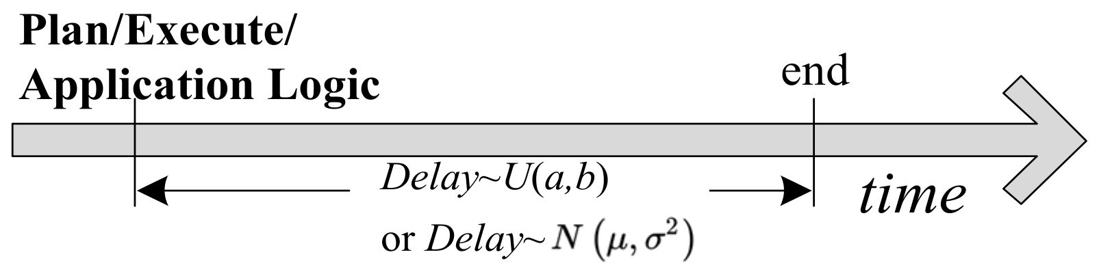
(Triggering-Delay Time ADelay). The Triggering-Delay Time refers to the time-interval of the Analyze process between when a monitoring variable is out of limits and when the subsequent Plan process is finally triggered. It is represented as ADelay, as shown in Figure 4.
In the SAS systems, when the monitoring variable v is detected out of limits (i.e., v > UpperLimit or v < LowerLimit in Figure 4), the Analyzer module will observe v continuously for a period of time, i.e., ADelay. If v still remains in the out-of-limit state (i.e., v > UpperLimit or v < LowerLimit), the subsequent Plan process would be triggered. Taking the adaptation scenario in Section 2.1 for example, as shown in Figure 5, the CPU utilization (i.e., the variable of Utilization) rises above its upper limit (i.e., 85%) at t1 and returns to its normal range at t2. As the out-of-limit time is less than ADelay (i.e., Δt1 = t2 − t1 < ADelay), there is no need to trigger further self-adaptation actions. However, this variable rises above its upper limit again at t3, and the out-of-limit time is longer than ADelay (i.e., Δt2 = t4 − t3 > ADelay). As a result, the subsequent processes would be triggered. The time constraint of Triggering-Delay Time is defined to specify such kind of delay-triggering self-adaptation strategies as, “if Utilization > UpperLimit for N seconds, then add P more VMs”. According to repeated experiments, ADelay takes the value of 3-unit time in the above example.
The time constraint of Triggering-Delay Time ADelay can effectively avoid system misjudgment and unnecessary self-adaptation actions. The value of ADelay should be set according to the concrete scenario, as the too large value would reduce the sensitivity and effectiveness of the self-adaptation logic, and the too-small value would result in over-frequent self-adaptation actions and aggravate the computing burden of the system.
4.1.2. Uncertainty Delay Time Constraints
The uncertainty delay time constraints mainly exist in the Plan process (i.e., DelayPlan), the Execute process (i.e., DelayExecute), and the application logic, and they come from a variety of sources, including the message processing, the network congestion of distributed systems, the algorithm running, the resource scheduling of large-scale systems, etc.
Despite the variety of causes, the uncertainty delay time can be represented as probability distribution functions. According to the Timed-SAS approach, the uncertainty delay time constraints are mainly represented as the Uniform Distribution function and the Normal Distribution function, as shown in Figure 6.
As for the SUIS example in Section 2.1, the uncertainty delay time constraints exist in the following aspects. Firstly, the running time of the self-adaptation strategies in the Plan process obeys the uniform distribution; secondly, the server scheduling time in the Execute process complies with the normal distribution; and finally, the networking delay time in the application logic obeys the uniform distribution. In the SUIS example, the uncertainty delay time constraints are set as follows, DelayPlan~U (1, 3), DelayExecute~N (5, 0.1) and DelayApp~U (1, 3).
4.1.3. Time Evaluation Metrics
The time evaluation metrics, i.e., Self-adaptive Adjusting Time and Self-adaptive Steady Time, are defined to evaluate the performance and response-time of the self-adaptation logic.
Definition 3.
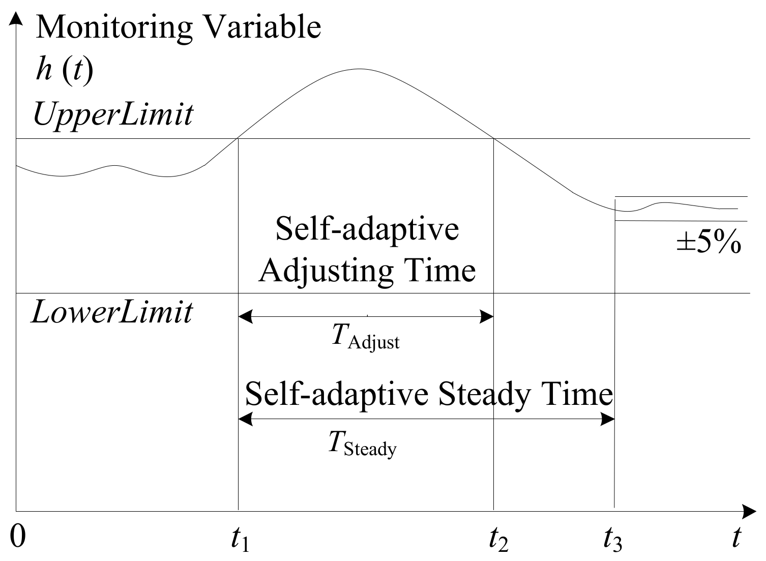
(Self-adaptive Adjusting Time TAdjust). The time evaluation metric of Self-adaptive Adjusting Time refers to the minimum time required for the SAS systems to recover from beyond the limits to within the limits. It is represented as TAdjust, as shown in Figure 7.
Definition 4.
(Self-adaptive Steady Time TSteady). The time evaluation metric of Self-adaptive Steady Time refers to the minimum time required for the SAS systems to recover to and maintain at the final value of ±5% after the limits being violated. It is represented as TSteady, as shown in Figure 7.
The two metrics are different, as TAdjust represents the response time to recover to safe states, while TSteady depicts the response time to recover to steady states.
In the SUIS example of Section 2.1, the monitoring variable is the CPU utilization. At time t1, the variable Util is detected exceeding the upper limit, and the subsequent self-adaptation strategies are triggered. Subsequently, the variable Util falls back to normal range at time t2, and returns to steady state at time t3. And the time of (t2–t1) is called Self-adaptive Adjusting Time, while the time of (t3–t1) is called Self-adaptive Steady Time. The two metrics can be used to evaluate the performance and response-time of the self-adaptation strategies.
4.2. Formal Modeling Templates and Application
In order to consolidate design knowledge for reuse, we create a set of formal modeling templates (https://github.com/DeshuaiHan/Timed-SAS-templates-and-examples) to describe the self-adaptation processes, the time behaviors and the uncertainty environment.
4.2.1. Templates for Self-Adaptation Processes and Time Behaviors
In the Timed-SAS approach, we use the NPTA model to depict the self-adaptation processes of “Monitor-Analyze-Plan-Execute”, use “declaration” to model the “Knowledge” module, and use “clock”, “guard” and “invariant” to specify the deterministic time constraints. The uncertainty delay time constraints are implemented in the “declaration” module.
Concretely, the modeling template for Monitor process and Monitoring Period MPeriod is shown in Figure 8a. It has decomposed the Monitor process into four sub-processes of “Timing, Data-Collection, Comparing, Triggering”. In the Timing sub-process, it has defined Monitoring Period by integrating invariant T < = Period with guard T == Period. In the Data-Collection sub-process, it uses the function getData( ) to detect the software running information. In the Comparing sub-process, it judges system states, low, high or NoChange, by comparing the monitoring variable with the upper and lower limit with the compare( ) function. Finally, it triggers different subsequent transitions by assigning different values to flagA. Notably, the implementation details of the above two functions are stored in the back-end configuration, which support customized definition according to the application scenarios.
The modeling template for Analyze process and Triggering-Delay Time ADelay is shown in Figure 8b. This process is triggered by flagA, and it is composed of three sub-processes of “Delaying-Comparing-Triggering”. In the process of Delaying, two Triggering-Delay Time D_T1 and D_T2 are defined. When the Triggering-Delay Time is finished and the monitored variable is still over-limit, the system state would be determined as “OverSatisfied” or “UnderSatisfied” with function analyze( ). Meanwhile, the flag of flagP would be assigned as −1 or 1, and the subsequent self-adaptation processes would be triggered. Similarly, the implementation details of analyze( ) need to be further customized.
The modeling template for Plan process and the uncertainty delay time DelayPlan is shown in Figure 8c. This process is triggered by flagP, and the concrete planning processes are implemented with two functions of plan_LCL( ) and plan_UCL( ), which need customization according to concrete applications. The uncertainty delay time is implemented with the function of delay(type, par1, par2), the parameters of which needs further instantiation.
Similarly, the template for Execute process and the uncertainty delay time DelayExecute is shown in Figure 8d. This process is triggered by flagE, and the executing processes are implemented with two functions of exe_LCL( ) and exe_UCL( ), which need further customization in the back-end configuration.
The uncertainty delay time constraints are implemented in the “declaration” module of NPTA, and Listing 1 provides the details. The function delay( ) defines types of probability distribution (from line 15 to line 20) for the delay time. When type == 1, the uncertainty delay time follows the normal distribution (from line 17 to line 18), while type == 2 follows the uniform distribution (from line 19 to line 20). The uniform distribution function (from line 9 to line 13) is created based on the UPPAAL-SMC built-in function of random ( ); while the normal distribution function (from line 5 to line 8) is implemented based on the standard normal distribution function (from line 1 to line 4), which is created using the Box–Muller method [24].
Listing 1. Implementation of the uncertainty delay time constraints in the SAS systems.
| 1 2 3 4 5 6 7 8 9 10 11 12 13 14 15 16 17 18 19 20 | // normal distribution for delay time N(0, 1) double stdNormal() { return sqrt(−2*ln(1-random(1)))*cos(2*PI*random(1)); } // normal distribution for delay time double Normal(double mean, double stdDev){ return mean + stdDev*stdNormal(); } // uniform distribution for delay time double Uniform(double min, double max){ … X = min + random(max–min); … // type of uncertainty delay time double delay (int type, double par1, double par2){ … if (type == 1) //N(par1, par2) … else if (type == 2) //U(par1, par2) … |
4.2.2. Templates for Uncertainty Environment
In order to simulate the dynamic software running environment, we created a template called Uncertainty Environment1, as shown in Figure 9. This modeling template describe two kinds of uncertainty, i.e., the stochastic software behaviors and the dynamic system loads. The former is handled with the probabilistic choices between multiple enabled transitions. As shown in Figure 9, there are five transitions following the state of “trigger”, and the transitions are executed with different probabilities, i.e., pr1, pr2, pr3, pr4, and pr5. While the latter is simulated with different kinds of functions. For example, transition (a) and (b), respectively, represent the linearly increasing and linearly decreasing monitored-variables; transition (d) and (e) respectively describe the sudden increase and decrease monitored variables; while transition (c) represents the periodical changing monitored variables.
The above formal modeling templates consolidate design knowledge of time behaviors and uncertainty environment for the SAS systems, and they can be customed and reused by users.
4.2.3. Application of the Formal Modeling Templates
By instantiating the modeling templates in Section 4.2.1 and Section 4.2.2, the formal model of the SUIS example was easily created. During the instantiation process, the front-end model in Figure 8 remained unchanged, the back-end functions and local variables of Monitor, Analyze, Plan, Execute, and Uncertainty Environment were customized according to the SUIS example. In addition, the application logic model of SUIS was newly created.
Concretely, in the processes of Monitor and Analyze, we mainly customized the functions of getData( ), compare( ) and analyze( ), and instantiated the Monitoring Period as const int Period = 5 (i.e., MPeriod =5), the Triggering-Delay Time as const int D_T1 = 3, D_T2 = 3 (i.e., ADelay = 3). In the processes of Plan and Execute, we mainly instantiated the uncertainty delay function of delay( ), except for customizing the functions of plan_LCL( ), plan_UCL( ), exe_LCL() and exe_UCL( ). As for Plan, the uncertainty delay time DelayPlan arised from the running time of the self-adaptation strategies, therefore, the parameter type in the delay function was set as Uni, i.e., the strategy running time obeys the uniform distribution, i.e., U (1, 3); while the uncertainty delay time in the Execute process (i.e., DelayExecute) was caused by server scheduling, thus, the parameter type was set as Norm, i.e., the server scheduling time follows the normal distribution, i.e., N (5, 0.1). As for the Uncertainty Environment template, it needed to simulate a Slashdot effect [16], thus, the parameters of pr1, pr2, pr3 and pr4 were set as 0, while pr5 = 1, which simulated a rapid increase of user visits (i.e., 42% increase of CPU Utilization). With the above templates, the self-adaptation strategy in Section 2.1 (i.e., if Utilization > UpperLimit for N seconds, then add P more VMs) can be implemented. In this strategy, “if Utilization > UpperLimit” was implemented with the Monitor process, “for N seconds” was implement with the time constraint of Triggering-Delay Time, and “add P more VMs” was implemented with the plan_UCL() function of Plan process and the exe_UCL() function of Execute process.
Except for instantiating the templates in Section 4.2.1 and Section 4.2.2, we constructed the application logic model for SUIS, as shown in Figure 10. It simulated the influence of server number changing on the CPU utilization. Combined with the user-customized application logic model, the self-adaptation loop became a closed feedback loop.
From the above example application, it can be seen that the created modeling templates can consolidate design knowledge for reuse, and thus reduce the modeling difficulty of the SAS systems.
4.3. Quantitative Analysis Templates and Application
4.3.1. Quantitative Analysis Templates
The traditional NTA-based SAS modeling framework and model checking technique suffer from the problem of state–space explosion during formal verification. The NPTA-based modeling templates and the SMC based quantitative analysis technique can avoid this problem. The quantitative analysis templates1 are shown in Table 1.
Concretely, the first property “self-adaptation reachability” is verified with the formal logic of “simulate [<=2T; N]{flagA}”, which checks whether the self-adaptation logic can be triggered during 2T time. If the self-adaptation logic is triggered after N times of simulation, the variable flagA would change from 0 to 1 or −1. The second property “self-adaptation strategy reachability” is used to verify whether the strategies can be triggered in response to the environment changes, and to compute the triggering probability and the average triggering time. The third to fifth properties are used to, respectively, analyze the Triggering-Delay Time, the Uncertainty Delay Time in Plan, and the Uncertainty Delay Time in Execute. The final property “Self-adaptive Adjusting Time and Self-adaptive Steady Time Analysis” is formally described as “simulate [<=Bound; N]{VAR}”, which simulates changes of the monitored variable. Furthermore, the users can identify the average Self-adaptive Adjusting Time and Self-adaptive Steady Time according to the formal logic of “Pr[<=Bound](<>VAR<=UCL) or Pr[<=Bound](<>VAR>=LCL)”.
4.3.2. Application of the Formal Analysis Templates
By instantiating the analysis templates in Section 4.3.1, the SUIS application was quantitatively verified and analyzed, and the results are shown in Figure 11. Concretely, the property of “self-adaptation reachability” was analyzed with the expression of “simulate [<=10; 10]{flagA}”. According to Figure 11a, the value of flagA turned from 0 to 1 at time 5, which meant the out-of-range CPU utilization (i.e., Util>=UCL) was detected after one cycle (i.e., Period = 5) of monitoring, and the self-adaptation logic was subsequently triggered. According to Figure 11b, the Plan.UCL_Plan state can be reached, which meant the self-adaptation strategy plan_UCL( ) was effectively executed at an average triggering time of 9.82. According to Figure 11c, the Analyze.analyze2 state can be reached at an average time of 8.80, which meant that the predefined Triggering-Delay Time (i.e., D_T2 = 3) was effective. According to Figure 11d,e, the processes of Plan and Execute can be reached, and the average finishing time were 11.8 and 18.0, respectively. Figure 11f shows that the CPU utilization fell in the normal range (i.e., Util < =85%) during the time of [16.44, 32.38], and the average Self-adaptive Adjusting Time was 21.20, which was analyzed with Pr[<=32](<>Util<=85); subsequently, it went through another times of self-adaptation and finally fell in the steady state during [22.24, 44.46], and the average Self-adaptive Steady Time was 30.30, which was analyzed with Pr[<=44](<>Util<=80).
For further analysis, on the basis of the above simulated values and the instantiated design values (i.e., the time features in Section 4.2.3), we plotted the timeline of the SUIS example, as shown in Figure 12. It shows that all the simulated values of the time behaviors fell in the design range. According to the above quantitative analysis, we can conclude that the self-adaptation behaviors, the self-adaptation strategies, and the time behaviors of the SUIS example were effective in dealing with the dynamic environment changes. Meanwhile, it can also be seen that the average Self-adaptive Steady Time was much longer than the average Self-adaptive Adjusting Time, and the number of servers in operation needed several times of adjustment, which indicated that current self-adaptation strategies were effective but not optimal.
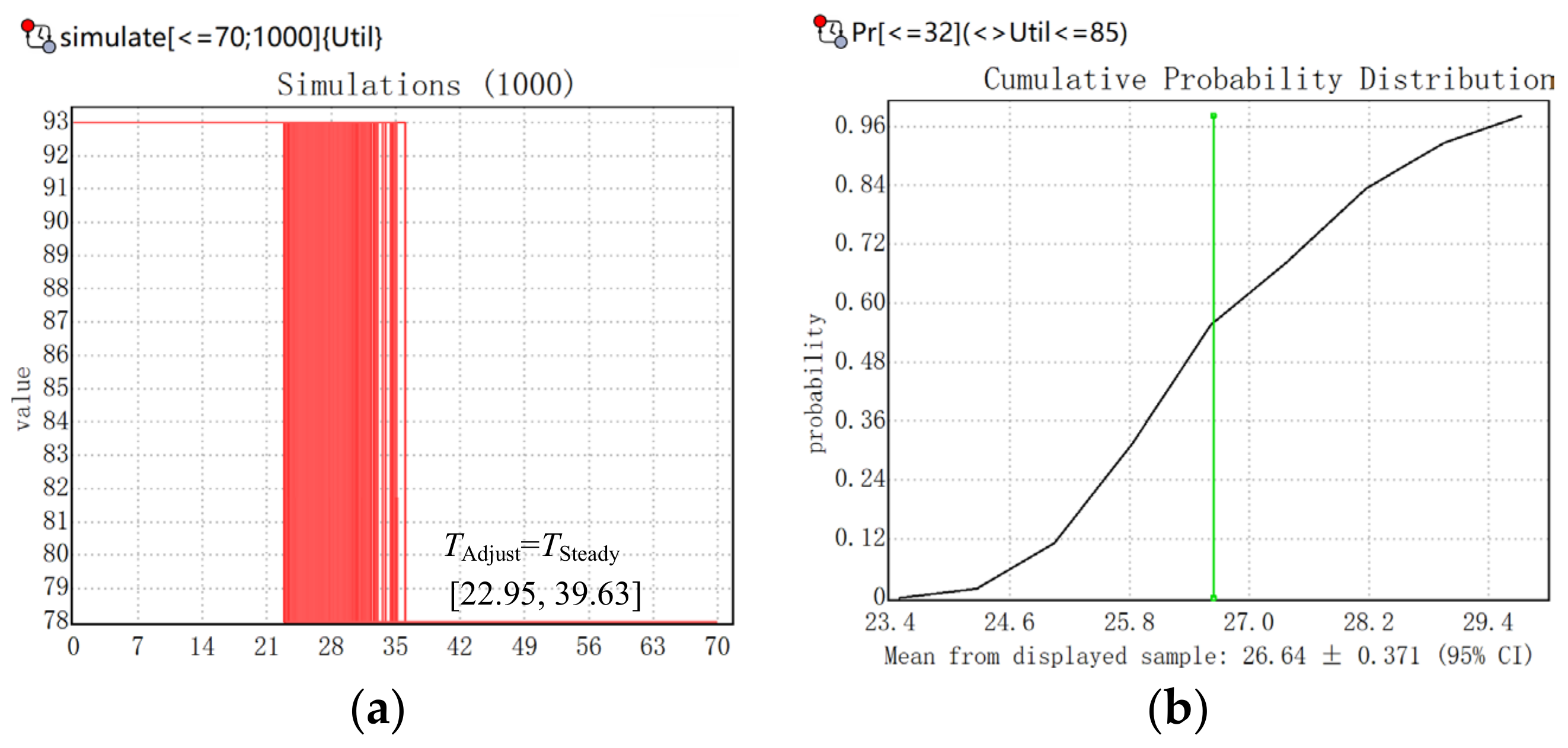
For further optimization, we have improved the self-adaptation strategy of “if Utilization > UCL for ADelay, then add P more VMs”, and adjusted the time constraints, as shown in Table 2. On one hand, the monitoring period, the server number P and the Triggering-Delay Time ADelay were optimized to avoid the repeated adjustment of the server number in operation. On the other hand, the delay time in the Plan and Execute processes were optimized to shorten the Self-adaptive Adjusting Time. The system behaviors after optimization are shown in Figure 13. As can be seen from Figure 13a, the number of servers in operation only went through one time of adjustment, and thus the Self-adaptive Adjusting Time was equal to the Self-adaptive Steady Time. In addition, the average Self-adaptive Steady Time was shortened to 26.64, compared with the initial model, as shown in Figure 13b. Back to the SUIS example in Section 2.1, the self-adaptation strategy can be optimized as “if Util > 85% for 16 unit time, then add ((Util−0.25)/5 + 2) more VMs”.
As can be seen from the above example application, the created quantitative analysis templates are effective in analyzing the self-adaptation properties as well as the time properties of the SAS systems. In addition, the templates can help to optimize the self-adaptation logic.
5. Experiment Evaluation
The objective of this experiment was to evaluate the effectiveness and efficiency of the templates created in the Timed-SAS approach. The effectiveness was examined from the reusability of the modeling and analysis templates, while the efficiency was evaluated from the modeling and analysis time of the SAS applications.
5.1. Experiment Setting
The experiment was performed in the context of a graduate course called ‘Advanced Software Engineering’ at Rocket Force University of Engineering, and the participants were 20 graduate students taking the course. The participants were randomly divided into five groups, and each group was randomly divided into two sub-groups, A and B. During the experiment, the participants were asked to finish modeling and formal analysis of five classical SAS applications, i.e., Body Sensor Network [25], Fire Detection System [18], Znn.com [20], Lon893OPCServer [26], and SUIS in Section 2.1.
According to the experiment design in Table 3, the experiment was carried out following five steps. In the first step, all the 20 participants equally received a 2-h lecture on the SAS systems and the MAPE-K architecture. Then, they were trained in a 6-h course to understand and to use the NPTA model and the UPPAAL-SMC tool. Notably, none of them was trained with the Timed-SAS approach in the above training. In the third step, each group selected one SAS application at random. The selection results were shown in Table 3, with specific modeling and analysis requirements set for each SAS application (https://github.com/DeshuaiHan/Timed-SAS-templates-and-examples). In the subsequent fourth step, each group was asked to finish modeling and formal analysis of the corresponding application in 4 h. Among each of the groups, Sub-group A was asked to use the templates created in the Timed-SAS approach, while Sub-group B was asked to directly use the NPTA model. Finally, in the fifth step, two teachers, who were not involved in the Timed-SAS project, were asked to check the finished tasks according to a set of concrete criteria (https://github.com/DeshuaiHan/Timed-Timed-SAS-experiment-evaluation).
5.2. Experiment Results and Discussion
After the experiment, we obtained two set of results for each example application (https://github.com/DeshuaiHan/Timed-Timed-SAS-experiment-evaluation). Due to space limitations, we only present the analysis results for each case study.
5.2.1. Data Analysis
According to the checking results of two teachers, Table 4 and Table 5 were created. As shown in Table 4, Sub-group A of the five groups, who used the templates of the Timed-SAS approach, all finished modeling and formal analysis of the specified SAS applications, and the average working time was 60.2 min. As for Sub-group B, who directly used the NPTA model, three of five sub-groups (i.e., Group 1-B, Group 2-B and Group 4-B) finished the specific tasks, and the average finishing time was 155.3 min. The other two sub-groups failed in the specific tasks because of timeout (i.e., Group 3-B) or unqualified work (i.e., Group 5-B).
Table 5 details the reusability for each template created in the Timed-SAS approach. Notably, all the templates were reused in three applications (i.e., the application of Znn.com, Lon893OPCServer and SUIS). For the above three applications, the templates were directly reused after modifying parameters. In the application of Fire Detection System, the Uncertainty Environment template was not useful, as the danger of fire was a determined value of 0 or 1. In the application of Fire Detection System and Body Sensor Network, the Self-adaptive Steady Time Analysis template was not useful, as the two systems were not closed loop feedback systems. In addition, the NTA model for Fire Detection System in Figure 14, was an instantiated and simplified version of the templates in Figure 8. From the above application and instantiation, we can conclude that the templates created in Timed-SAS can cover modeling and formal analysis requirements of the five example applications.
5.2.2. Experiment Results
Considering the experiment objective mentioned at the beginning of this experiment, i.e., evaluating the effectiveness and efficiency of the templates created in the Timed-SAS approach, we discuss the experiment results in this subsection.
Effectiveness. The effectiveness is examined from the template reusability. According to Table 4 and Table 5, the templates created in the Timed-SAS approach can be directly instantiated and reused and can satisfy the modeling and formal analysis requirements of the general SAS systems. In addition, from the application in Section 4.2.3 and Section 4.3.2, it can be seen that the templates help to reduce modeling and formal verification difficulties of the time behaviors, and to optimize the self-adaptation logic. Thus, the templates created in the Timed-SAS approach are effective.
Efficiency. Similarly, the efficiency depends on the formal modeling and analysis time with the templates. According to Table 4, the average working time when using the templates was shortened by 61.24%, compared with directly using the NPTA model. Thus, the Timed-SAS approach has a distinct advantage in improving the formal modeling and analysis efficiency of the SAS time behaviors.
5.2.3. Discussion
Strengths. The above experiment evaluation has demonstrated that the templates created in the Timed-SAS approach are effective to describe and analyze the self-adaptation processes, the time behaviors, and the uncertainty environment of the SAS systems. The templates can help to reduce formal modeling and analysis difficulties and improve the modeling and analysis efficiency of the SAS systems.
Weakness. The experiment evaluation also reveals one deficiency of the Timed-SAS approach. Currently, the NPTA model still lacks an effective mechanism to handle high system complexity. To make up for this deficiency, we made a preliminary study [21] with the stepwise refinement mechanism of the Event-B model [27]. In future work, we will attempt to integrate the Timed-SAS approach with the Event-B model.
5.3. Threats to Validity
The validity of our controlled experiments may be subject to the following threats:
Construct validity. This kind of validity analyzes the relationship between theory and observation. The above experiment was conducted to evaluate the effectiveness and efficiency of the created templates. The concepts of “effectiveness” and “efficiency” are broad and general and are prone to construct validity. To minimize this threat, the effectiveness was examined from the template reusability, and the corresponding evaluation metrics were concrete and quantifiable; while the efficiency was evaluated with the modeling and analysis time of the SAS applications, which was also a quantitative metric.
Internal validity. As for internal validity, the manual assessment of tasks in the fifth step of the experiment (i.e., results analysis in Table 3) is prone to errors and bias. To reduce this kind of threat, the task assessment was conducted by two domain experts who were not directly involved in our project. In addition, the assessment followed a blind procedure.
External validity. External validity refers to the generalizability of the experiment conclusions. In this study, we performed the experiments with five classical self-adaptive software scenarios, and the experiment results are satisfactory. However, the backgrounds of the experiments’ subjects are limited. In the above experiments, we chose 20 graduate students as subjects, but the modeling and quantitative analysis templates of the Timed-SAS approach is designed not only for students but also for industrial software developers. In the future, we plan to conduct more experiments with subjects from the industrial community.
6. Related Work and Discussion
Recently, the study on the SAS systems has become a hot topic in the software engineering community. Particularly, formal methods for the SAS systems are attracting increasing interest. The self-adaptive software community has made several comprehensive surveys [28,29,30], focusing on modeling dimensions, engineering approaches and formal methods of self-adaptive systems, respectively. This study focuses on formal modeling and analysis of the self-adaptation processes and the time behaviors for the SAS systems, and we review studies that are relevant to our Timed-SAS approach.
Formal modeling and verification on the self-adaptation processes. In order to formally describe and verify the self-adaptation processes, researchers have proposed many approaches, such as the CSP-based approaches [31,32], the Petri-Net based approaches [33,34], the NTA-based approaches [10,11,12], the Event-B based approaches [18,21,35], the approaches based on domain specific language [36,37], etc. One popular approach is the NTA-based approach, owing to its simplicity and ease-of-use features. On basis of the timed automata model, the AdaptWise research group of Linnaeus University proposed the ActivFORMS approach [10], the MAPE-K formal templates [11], and the eARF approach [12] for the SAS systems. The above research concentrates on formal modeling and verification of the dynamic self-adaptation processes, but they lack a systematic definition and description on the time behaviors within the SAS systems. In addition, model checking of the above formal models encounters the problem of state–space explosion when system scales increase. By contrast, our Timed-SAS approach provides a systematic definition on the time behaviors within the SAS systems and supports formal modeling and quantitative analysis of the dynamic self-adaptation processes as well as the time behaviors. Furthermore, the Timed-SAS approach can avoid the state–space explosion problem with the Statistical Model Checking technique.
Formal modeling and verification on the time behaviors of the SAS systems. Time behavior is an important characteristic for the self-adaptive systems. Ji Zhang and BHC Cheng [38] have long pointed out the need to specify the adaptation requirements with temporal logic. Furthermore, they have proposed the Adapt operator-extended LTL (A-LTL) [39] to specify adaptation semantics. Similarly, Zhao et al. [40] have proposed the mode-supported Linear Temporal Logic (mLTL) to specially describe global specifications of the self-adaptive software. The above studies have treated time behaviors as first-class elements to handle, but they lack a systematic definition on the time behaviors within the SAS systems. As for definitions on the time behaviors, the authors in [18] defined the time behaviors of deadline, delay, and expiry for the self-adaptive systems. On the basis of these definitions, the authors proposed to extend the Event-B model with timing semantics, and defined the refinement patterns for deadline, delay and expiry, which can reduce modeling difficulties of time behaviors. Unfortunately, the above modeling patterns cannot describe the time behaviors under uncertainty environment. Apart from definitions on the deterministic time behaviors, we have defined the uncertainty time behaviors to describe the delay time under uncertainty environment.
Quantitative analysis on the SAS systems. In order to quantitatively analyze the system behaviors under uncertainty, the researchers have proposed the Probabilistic Model Checking based approaches [41,42,43,44] for the SAS systems. These approaches possess the advantages of automatic analysis and quantitative verification and can avoid the state–space explosion problem of model checking. However, there is still a lack of quantitative metrics to evaluate the self-adaptation logic [45]. To make up for this deficiency, we proposed the metrics of Self-adaptive Steady Time and Self-adaptive Adjusting Time, which can be used to quantitatively evaluate the performance and response time of the self-adaptation logic. Furthermore, on the basis of the Statistical Model Checking technique, we created a set of quantitative analysis templates to analyze the self-adaptation properties and the time properties under uncertainty.
To summarize, our work concentrated on definition, formal modeling and quantitative analysis of the self-adaptation processes and the time behaviors for the SAS systems. To the best of our knowledge, this is the first attempt to systematically tackle the time behaviors within the SAS systems.
7. Conclusions and Future Work
Formal modeling and quantitative analysis of time behaviors is of vital importance for the SAS systems. However, few studies have systematically considered the time behaviors, especially the uncertainty delay time constraints within the self-adaptation loops. To this end, the Timed-SAS approach, which supports definition, formal modeling, quantitative analysis and optimization for the time behaviors of the SAS systems, was proposed in this paper. The Timed-SAS approach was created based on the commonly used MAPE-K self-adaptive software architecture, and its contribution is two-fold: the approach provides a systematical definition on the time constraints within each MAPE-K process and on the time-based evaluation metrics for the self-adaptation loops, and presents a set of formal modeling templates and quantitative analysis templates for the time behaviors within the SAS systems. The defined time constraints can be used to depict the deterministic time constraints, and the uncertainty time constraints within the self-adaptation processes; the time-based evaluation metrics can be used to evaluate the performance and response-time of the self-adaptation loops and the self-adaptation strategies; and the modeling and quantitative analysis templates can consolidate design knowledge for reuse, and can alleviate modeling difficulty and improve modeling efficiency of the SAS systems. Furthermore, the Timed-SAS approach can be used to optimize the self-adaptation strategies of the SAS systems. We evaluated the Timed-SAS approach with several example applications and a subject-based experiment. The results demonstrated that the Timed-SAS approach can satisfy modeling requirements of the SAS time behaviors, and effectively reduce the modeling and quantitative analysis difficulty of the SAS time behaviors.
In future work, we will continue to study the formal analysis of self-adaptation properties, simplify the quantitative analysis complexity and enrich the verifiable self-adaptation properties.
Author Contributions
Conceptualization, D.H. and Y.C.; methodology, D.H.; software, W.C.; validation, W.C.; formal analysis, D.H.; data curation, W.C.; writing—original draft preparation, D.H. and Z.C.; writing—review and editing, D.H. and Y.C.; visualization, Z.C.; supervision, A.L.; project administration, D.H. All authors have read and agreed to the published version of the manuscript.
Funding
This research was funded by Natural Science Basic Research Plan in Shaanxi Province of China (Program No. 2021JQ-374).
Institutional Review Board Statement
Not applicable.
Informed Consent Statement
Not applicable.
Data Availability Statement
The datasets generated during and/or analyzed during the current study are available from the corresponding author on reasonable request.
Conflicts of Interest
The authors declare no conflict of interest.
References
- Chen, X.; Wang, H.; Ma, Y.; Zheng, X.; Guo, L. Self-adaptive resource allocation for cloud-based software services based on iterative QoS prediction model. Future Gener. Comput. Syst. 2020, 105, 287–296. [Google Scholar] [CrossRef]
- Gerostathopoulos, I.; Bures, T.; Hnetynka, P.; Keznikl, J.; Kit, M.; Plasil, F.; Plouzeau, N. Self-adaptation in software-intensive cyber–physical systems: From system goals to architecture configurations. J. Syst. Softw. 2016, 122, 378–397. [Google Scholar] [CrossRef]
- Salehie, M.; Tahvildari, L. Self-adaptive software: Landscape and research challenges. ACM Trans. Auton. Adapt. Syst. TAAS 2009, 4, 14. [Google Scholar] [CrossRef]
- Weyns, D. Software engineering of self-adaptive systems. In Handbook of Software Engineering; Cha, S., Taylor, R.N., Kang, K., Eds.; Springer: Berlin/Heidelberg, Germany, 2019; pp. 399–443. [Google Scholar]
- Abbas, N.; Andersson, J.; Weyns, D. ASPLe: A methodology to develop self-adaptive software systems with systematic reuse. J. Syst. Softw. 2020, 167, 110626. [Google Scholar] [CrossRef]
- Kephart, J.O.; Chess, D.M. The vision of autonomic computing. Computer 2003, 36, 41–50. [Google Scholar] [CrossRef]
- Fülöp, E.; Pataki, N. A DSL for resource checking using finite state automaton-driven symbolic execution. Open Comput. Sci. 2021, 11, 107–115. [Google Scholar] [CrossRef]
- Fernandes Costa, T.; Sobrinho, Á.; Chaves e Silva, L.; da Silva, L.D.; Perkusich, A. Coloured Petri Nets-Based Modeling and Validation of Insulin Infusion Pump Systems. Appl. Sci. 2022, 12, 1475. [Google Scholar] [CrossRef]
- Weyns, D.; Bencomo, N.; Calinescu, R.; Cámara, J.; Ghezzi, C.; Grassi, V.; Grunske, L.; Inverardi, P.; Jézéquel, J.-M.; Malek, S.; et al. Assurances for Self-Adaptive Systems; Springer: Berlin/Heidelberg, Germay, 2017. [Google Scholar]
- Weyns, D.; Iftikhar, M.U. ActivFORMS: A Model-Based Approach to Engineer Self-Adaptive Systems. IEICE Trans. Fundam. Electron. Commun. Comput. Sci. 2019, 2019, 3522585. [Google Scholar] [CrossRef]
- Iglesia, D.G.D.L.; Weyns, D. MAPE-K formal templates to rigorously design behaviors for self-adaptive systems. ACM Trans. Auton. Adapt. Syst. 2015, 10, 2724719. [Google Scholar] [CrossRef]
- Abbas, N.; Andersson, J.; Iftikhar, M.U.; Weyns, D. Rigorous architectural reasoning for self-adaptive software systems. In Proceedings of the 1st Workshop on Qualitative Reasoning about Software Architectures, Venice, Italy, 5–8 April 2016; pp. 11–18. [Google Scholar]
- Bulychev, P.; David, A.; Larsen, K.G.; Mikučionis, M.; Poulsen, D.B.; Legay, A.; Wang, Z. UPPAAL-SMC: Statistical model checking for priced timed automata. arXiv 2012, arXiv:1207.1272. [Google Scholar] [CrossRef] [Green Version]
- Sen, K.; Viswanathan, M.; Agha, G. Statistical model checking of black-box probabilistic systems. In Proceedings of the International Conference on Computer Aided Verification, Boston, MA, USA, 13–17 July 2004; Springer: Berlin/Heidelberg, Germany, 2004; pp. 202–215. [Google Scholar]
- Han, D.; Xing, J.; Yang, Q.; Li, J.; Wang, H. Handling uncertainty in self-adaptive software using self-learning fuzzy neural network. In Proceedings of the IEEE Computer Society, Proceedings of the 40th IEEE Annual Computer Software and Applications Conference (COMPSAC), Atlanta, GA, USA, 10–14 June 2016; pp. 540–545. [Google Scholar]
- Adler, S. The Slashdot Effect: An Analysis of Three Internet Publications. Linux Gazette. 1999, p. 38. Available online: https://linuxgazette.net/issue38/adler1.html (accessed on 29 January 2023).
- Arcaini, P.; Riccobene, E.; Scandurra, P. Modeling and analyzing MAPE-K feedback loops for self-adaptation. In Proceedings of the 10th IEEE/ACM International Symposium on Software Engineering for Adaptive and Self-Managing Systems, Florence, Italy, 18–19 May 2015; pp. 13–23. [Google Scholar]
- Hachicha, M.; Halima, R.B.; Kacem, A.H. Design and timed verification of self-adaptive systems. In Proceedings of the IEEE/ACIS 16th International Conference on Computer and Information Science (ICIS), Wuhan, China, 24–26 May 2017; pp. 227–232. [Google Scholar]
- Han, D.; Yang, Q.; Xing, J.; Li, J.; Wang, H. FAME: A UML-based framework for modeling fuzzy self-adaptive software. Inf. Softw. Technol. 2016, 76, 118–134. [Google Scholar] [CrossRef]
- Cheng S, W. Rainbow: Cost-Effective Software Ar-Chitecture-Based Self-Adaptation; Carnegie Mellon University: Pittsburgh, PA, USA, 2008. [Google Scholar]
- Han, D.S.; Yang, Q.L.; Xing, J.C.; Ma, G.L. EasyModel: A Refinement-Based Modeling and Verification Approach for Self-Adaptive Software. J. Comput. Sci. Technol. 2020, 35, 1016–1046. [Google Scholar] [CrossRef]
- David, A.; Larsen, K.G.; Legay, A.; Mikučionis, M.; Poulsen, D.B. Uppaal SMC tutorial. Int. J. Softw. Tools Technol. Transf. 2015, 17, 397–415. [Google Scholar] [CrossRef]
- Larsen, K.G.; Pettersson, P.; Yi, W. UPPAAL in a nutshell. Int. J. Softw. Tools Technol. Transf. 1997, 1, 134–152. [Google Scholar] [CrossRef]
- Chen, M.; Yue, D.; Qin, X.; Fu, X.; Mishra, P. Variation-aware evaluation of MPSoC task allocation and scheduling strategies using statistical model checking. In Proceedings of the 2015 IEEE Design, Automation & Test in Europe Conference & Exhibition (DATE), Grenoble, France, 9–13 March 2015; pp. 199–204. [Google Scholar]
- Rodrigues, A.; Rodrigues, G.N.; Knauss, A.; Ali, R.; Andrade, H. Enhancing context specifications for dependable adaptive systems: A data mining approach. Inf. Softw. Technol. 2019, 112, 115–131. [Google Scholar] [CrossRef]
- Yang, Q.L.; Lv, J.; Tao, X.P.; Ma, X.X.; Xing, J.C.; Song, W. Fuzzy self-adaptation of mission-critical software under uncertainty. J. Comput. Sci. Technol. 2013, 28, 165. [Google Scholar] [CrossRef]
- Abrial J, R. Modeling in Event-B: System and Software Engineering; Cambridge University Press: Cambridge, UK, 2013. [Google Scholar]
- De Lemos, R.; Garlan, D.; Ghezzi, C.; Giese, H.; Andersson, J.; Litoiu, M.; Schmerl, B.; Weyns, D.; Baresi, L.; Bencomo, N.; et al. Software engineering for self-adaptive systems: Research challenges in the provision of assurances. In Proceedings of the Software Engineering for Self-Adaptive Systems III, Wadern, Germany, 15–19 December 2013; Springer: Berlin/Heidelberg, Germany, 2017; Volume 9640. [Google Scholar]
- Krupitzer, C.; Roth, F.M.; VanSyckel, S.; Schiele, G.; Becker, C. A survey on engineering approaches for self-adaptive systems. Pervasive Mob. Comput. 2015, 17, 184–206. [Google Scholar] [CrossRef]
- Krupitzer, C.; Roth, F.M.; VanSyckel, S.; Schiele, G.; Becker, C. A survey of formal methods in self-adaptive systems. In Proceedings of the Fifth International C* Conference on Computer Science and Software Engineering, Guilin, China, 21–23 October 2022; pp. 67–79. [Google Scholar]
- Göthel, T.; Jähnig, N.; Seif, S. Refinement-based modelling and verification of design patterns for self-adaptive systems. In Proceedings of the 19th International Conference on Formal Engineering Methods, Xi’an, China, 13–17 November 2017; Springer: Berlin/Heidelberg, Germany; pp. 157–173. [Google Scholar]
- Kleine, M. A CSP-based framework for the specification, verification, and implementation of adaptive systems. In Proceedings of the 6th International Symposium on Software Engineering for Adaptive and Self-Managing Systems, Honolulu, HI, USA, 23–24 May 2011; 2011; pp. 158–167. [Google Scholar]
- Ding, Z.; Zhou, Y.; Zhou, M. Modeling self-adaptive software systems with learning petri nets. IEEE Trans. Syst. Man Cybern. Syst. 2017, 46, 483–498. [Google Scholar] [CrossRef]
- Kachi, F.; Bouanaka, C.; Merkouche, S. A formal model for quality-driven decision making in self-adaptive systems. In Proceedings of the Second Workshop on Formal Methods for Autonomous Systems, Constantine, Algirea, 7 December 2020; pp. 48–64. [Google Scholar]
- Su, W. Modeling of timing constraints in hybrid systems using Event-B. IEEE Trans. Reliab. 2020, 69, 581–593. [Google Scholar] [CrossRef]
- Arcaini, P.; Mirandola, R.; Riccobene, E.; Scandurra, P. MSL: A pattern language for engineering self-adaptive systems. J. Syst. Softw. 2020, 164, 110558. [Google Scholar] [CrossRef]
- Vogel, T. Model-Driven Engineering of Self-Adaptive Software; University of Potsdam: Potsdam, Germany, 2018. [Google Scholar]
- Zhang, J.; Cheng, B.H.C. Model-based development of dynamically adaptive software. In Proceedings of the 28th International Conference On Software Engineering, Shanghai, China, 20–28 May 2006; pp. 371–380. [Google Scholar]
- Zhang, J.; Cheng, B.H.C. Using temporal logic to specify adaptive program semantics. J. Syst. Softw. 2006, 79, 1361–1369. [Google Scholar] [CrossRef]
- Zhao, Y.; Li, Z.; Shen, H.; Ma, D. Development of global specification for dynamically adaptive software. Computing 2013, 95, 785–816. [Google Scholar] [CrossRef]
- Calinescu, R.; Gerasimou, S.; Johnson, K.; Paterson, C. Using runtime quantitative verification to provide assurance evidence for self-adaptive software. In Proceedings of Software Engineering for Self-Adaptive Systems III, Wadern, Germany, 15–19 December 2013; Springer: Cham, Switzerland, 2017; pp. 223–248. [Google Scholar]
- Filieri, A.; Tamburrelli, G.; Ghezzi, C. Supporting self-adaptation via quantitative verification and sensitivity analysis at run time. IEEE Trans. Softw. Eng. 2015, 42, 75–99. [Google Scholar] [CrossRef]
- Jamshidi, P.; Cámara, J.; Schmerl, B.; Käestner, C.; Garlan, D. Machine learning meets quantitative planning: Enabling self-adaptation in autonomous robots. In Proceedings of the IEEE/ACM 14th International Symposium on Software Engineering for Adaptive and Self-Managing Systems (SEAMS), Montreal, QC, Canada, 25 May 2019; pp. 39–50. [Google Scholar]
- Gerasimou, S. Runtime Quantitative Verification of Self-Adaptive Systems; University of York: York, UK, 2016. [Google Scholar]
- Gerostathopoulos, I.; Vogel, T.; Weyns, D.; Lago, P. How do we evaluate self-adaptive software systems? In Proceedings of the 16th International Symposium on Software Engineering for Adaptive and Self-Managing Systems, Madrid, Spain, 23–24 May 2021; pp. 158–167. [Google Scholar]
Figure 1.
Architectural view of SUIS.

Figure 2.
An overview of the Timed-SAS approach.

Figure 3.
Monitoring Period MPeriod for Monitor.

Figure 4.
Triggering-Delay Time ADelay for Analyze.

Figure 5.
Analysis of Triggering-Delay Time ADelay.

Figure 6.
The uncertainty time behavior of Delay.

Figure 7.
Self-adaptive Adjusting Time and Self-adaptive Steady Time.

Figure 8.
The NPTA based modeling templates for the self-adaptation processes and time behaviors: (a) the template for Monitor process and Monitoring Period MPeriod; (b) The template for Analyze process and Triggering-Delay Time ADelay; (c) the template for Plan process and the uncertainty delay time; and (d) the template for Execute process and the uncertainty delay time.

Figure 9.
The NPTA-based modeling templates for Uncertainty Environment.

Figure 10.
The user customized application logic model for SUIS.

Figure 11.
Quantitative analysis of the SUIS example: (a) self-adaptation reachability analysis; (b) self-adaptation strategy reachability analysis; (c) Triggering-Delay Time Analysis; (d) Uncertainty Delay Time (Plan) Analysis; (e) Uncertainty Delay Time (Execute) Analysis; and (f) Self-adaptive Adjusting Time and Self-adaptive Steady Time Analysis.

Figure 12.
Time behavior analysis for the SUIS example.

Figure 13.
Time behaviors of the optimized SUIS application: (a) the changes of CPU utilization; and (b) the average value of TAdjust and TSteady.
Figure 13.
Time behaviors of the optimized SUIS application: (a) the changes of CPU utilization; and (b) the average value of TAdjust and TSteady.

Figure 14.
Modeling the Fire Detection System by reusing and simplifying the templates of Timed-SAS: (a) reusing the templates of Monitor and MPeriod; (b) reusing and simplifying the templates of Analyze and ADelay; (c) reusing and simplifying the templates of Plan and DelayPlan; and (d) reusing and simplifying the templates of Execute and DelayExecute.


Table 1.
Quantitative analysis templates for the SAS systems.
| NO. | Types | Description and Usage | Implementation |
|---|---|---|---|
| 1 | Self-adaptation reachability | Analyzing if the self-adaptation logic can be triggered, and the triggering time. | simulate [<=2T; N]{flagA} |
| 2 | Self-adaptation strategy reachability | Analyzing if the corresponding self-adaptation strategies can be triggered, and the triggering probability and the average triggering time. | Pr[<=Bound](<>Plan.LCL_Plan) Pr[<=Bound](<>Plan.UCL_Plan) |
| 3 | Triggering-Delay Time (ADelay) Analysis | Analyzing whether the predefined Triggering-Delay Time is effective. | Pr[<=Bound](<>Analyze.analyze1) Pr[<=Bound](<>Analyze.analyze2) |
| 4 | Uncertainty Delay Time (DelayPlan) Analysis | Analyzing the total average delay time when finishing the Plan process, and the triggering probability. | Pr[<=Bound](<>Plan.PlanReady1) Pr[<=Bound](<>Plan.PlanReady2) |
| 5 | Uncertainty Delay Time (DelayExecute) Analysis | Analyzing the total average delay time when finishing the Execute process, and the triggering probability. | Pr[<=Bound](<> Execute.end) |
| 6 | Self-adaptive Adjusting Time and Self-adaptive Steady Time Analysis | Analyzing the effectiveness of the self-adaptation logic, the average time used to get back to normal and steady states, and the probabilities to get back to normal states within a given time limit. | simulate [<=Bound; N]{VAR} Pr[<=Bound](<>VAR<=UCL) Pr[<=Bound](<>VAR>=LCL) |
Table 2.
Optimization of self-adaptation strategies and time behaviors.
| Initial Parameter Configurations | Optimized Parameter Configurations |
|---|---|
| P = (Util-UCL)/5 + 1 | P = (Util-UCL)/5 + 2 |
| MPeriod = 5 | MPeriod = 2 |
| ADelay = 3 | ADelay = 16 |
| DelayPlan~U(1.0, 3.0) | DelayPlan~U(1.0, 2.0) |
| DelayExecute~ N(5.0, 0.1) | DelayExecute~ N(2.0, 0.1) |
Table 3.
Design of the experiment.
| Steps | Group 1 (A, B) | Group 2 (A, B) | Group 3 (A, B) | Group 4 (A, B) | Group 5 (A, B) |
|---|---|---|---|---|---|
| 1st Step: SAS training | Lectures on the SAS systems and the MAPE-K architecture (2 h) | ||||
| 2nd Step: Formal method training | Training on the NPTA formal model and the UPPAAL-SMC tool (6 h) | ||||
| 3rd Step: Application selection | Znn.com [20] | Lon893OPCServer [26] | Body Sensor Network [25] | Fire Detection System [18] | SUIS |
| 4th Step: Formal modeling and analysis | Formal modeling and analysis with the Timed-SAS approach and the NPTA model, respectively (limited in 4 h) | ||||
| 5th Step: Results analysis | Checking the modeling and formal analysis results (i.e., work quality, finishing time, and template reusability). | ||||
Table 4.
The finishing time and work quality for each case study.
| SAS Applications | Modeling and Analysis with the Timed-SAS Approach | Modeling and Analysis with the NPTA Model |
|---|---|---|
| Znn.com [20] | 63 min (Group 1-A) | 195 min (Group 1-B) |
| Lon893OPCServer [26] | 52 min (Group 2-A) | 163 min (Group 2-B) |
| Body Sensor Network [25] | 75 min (Group 3-A) | /(Group 3-B) (out range of 4 h) |
| Fire Detection System [18] | 45 min (Group 4-A) | 108 min (Group 4-B) |
| SUIS | 66 min (Group 5-A) | /(Group 5-B) (105 min, but unqualified) |
| Average time | 60.2 min | 155.3 min |
Table 5.
The template reusability for each example application.
| SAS Applications | MAPE-K | Uncertainty | MPeriod | ADelay | DelayPlan | DelayExecute | TAdjust | TSteady | SAS Reachability | Strategy Reachability |
|---|---|---|---|---|---|---|---|---|---|---|
| Znn.com [20] | √ | √ | √ | √ | √ | √ | √ | √ | √ | √ |
| Lon893OPCServer [26] | √ | √ | √ | √ | √ | √ | √ | √ | √ | √ |
| Body Sensor Network [25] | √ | √ | √ | √ | √ | √ | √ | -- | √ | √ |
| Fire Detection System [18] | √ | -- | √ | √ | √ | √ | √ | -- | √ | √ |
| SUIS | √ | √ | √ | √ | √ | √ | √ | √ | √ | √ |
| Number of uses | 5/5 | 4/5 | 5/5 | 5/5 | 5/5 | 5/5 | 5/5 | 4/5 | 5/5 | 5/5 |
Note: 1. MAPE-K: Modeling templates for MAPE-K processes; 2. Uncertainty: Modeling templates for uncertainty environment; 3. MPeriod: Modeling and analysis templates for MPeriod; 4. ADelay: Modeling and analysis templates for ADelay; 5. DelayPlan:Modeling and analysis templates for DelayPlan; 6. DelayExecute: Modeling and analysis templates for DelayExecute; 7. TAdjust: Modeling and analysis templates for TAdjust; 8. TSteady: Modeling and analysis templates for TSteady; 9. SAS reachability: Self-adaptation reachability analysis; 10. Strategy reachability: Self-adaptation reachability analysis. √: shows that the template is useful in the example. --: shows that the template is not useful in the example.
Disclaimer/Publisher’s Note: The statements, opinions and data contained in all publications are solely those of the individual author(s) and contributor(s) and not of MDPI and/or the editor(s). MDPI and/or the editor(s) disclaim responsibility for any injury to people or property resulting from any ideas, methods, instructions or products referred to in the content. |
© 2023 by the authors. Licensee MDPI, Basel, Switzerland. This article is an open access article distributed under the terms and conditions of the Creative Commons Attribution (CC BY) license (https://creativecommons.org/licenses/by/4.0/).
Share and Cite
MDPI and ACS Style
Han, D.; Cai, Y.; Chen, W.; Cui, Z.; Li, A. Timed-SAS: Modeling and Analyzing the Time Behaviors of Self-Adaptive Software under Uncertainty. Appl. Sci. 2023, 13, 2018. https://doi.org/10.3390/app13032018
AMA Style
Han D, Cai Y, Chen W, Cui Z, Li A. Timed-SAS: Modeling and Analyzing the Time Behaviors of Self-Adaptive Software under Uncertainty. Applied Sciences. 2023; 13(3):2018. https://doi.org/10.3390/app13032018
Chicago/Turabian StyleHan, Deshuai, Yanping Cai, WenJie Chen, Zhigao Cui, and Aihua Li. 2023. "Timed-SAS: Modeling and Analyzing the Time Behaviors of Self-Adaptive Software under Uncertainty" Applied Sciences 13, no. 3: 2018. https://doi.org/10.3390/app13032018
Note that from the first issue of 2016, this journal uses article numbers instead of page numbers. See further details here.