
A New Effective Narrowband Active Noise Control System for Accommodating Frequency Mismatch

1
School of Computer and Electronic Information/School of Artificial Intelligence, Nanjing Normal University, Nanjing 210023, China
2
Key Laboratory of Virtual Geographic Environment, Nanjing Normal University, Ministry of Education, Nanjing 210023, China
3
State Key Laboratory Cultivation Base of Geographical Environment Evolution (Jiangsu Province), Nanjing 210023, China
4
Jiangsu Center for Collaborative Innovation in Geographical Information Resource Development and Application, Nanjing 210023, China
*
Author to whom correspondence should be addressed.
Appl. Sci. 2023, 13(4), 2416; https://doi.org/10.3390/app13042416
Submission received: 30 November 2022
/
Revised: 8 February 2023
/
Accepted: 10 February 2023
/
Published: 13 February 2023
(This article belongs to the Special Issue Active Vibration and Noise Control)
Abstract
:Narrowband active noise control (NANC) has shown excellent performance in dealing with the low frequency periodic noise generated by rotating machines, such as fans, engines and power transformers. Accommodating large frequency mismatch (FM) and improving its tracking capability is required for the NANC system. The existence of FM influences the noise cancellation performance. In this paper, a frequency correction algorithm based on least mean p-power (LMP) combined with the autoregressive (AR) model is designed for the NANC system, which is simple and feasible, and has a good performance under a large step size. In the NANC system, the reference signal is handled by a delay unit and AR model, and the coefficients of the AR model are adjusted by the LMP algorithm, which fine-tunes the coefficients and offers the reference signals to the NANC system. The stability bounds for the step size parameter have also been derived in the mean sense. The designed mechanism converges fast and enhances the noise decrement. Extensive simulations are performed to demonstrate the superior performance of the proposed NANC in dealing with periodic noises.
1. Introduction
In our daily work and life, many disturbing noises can not only cause psychological discomfort for humans, but could also strengthen the structural load and, hence, give rise to fatigue damage [1,2,3,4,5]. These noises are generated by rotating machines such as cutting machines, electric fans, and motors. The other characteristic low frequency humming noise is due to the periodic vibration of the iron core with the change of the excitation frequency in the power transformer box [6]. A similar noise to this may be modeled as a sinusoidal signal in additive noise. Usually, the frequencies of the noise signals are arbitrary, and their magnitudes are time-varying. The noise generated by rotating or reciprocating equipment is mainly low frequency harmful noise [7]. Narrowband active noise control (NANC) is commonly used in noise-cancelling headsets [8,9], modern automobiles [10,11,12,13], and vehicle noise [14,15,16]. The conventional NANC system has shown great superiority in low frequency signal processing [17], while the use of sound-absorbing and sound-insulating materials shows a poor performance in dealing with the low frequency part of this noise [18].
In general, there are two ways to obtain reference signals. One is to obtain the noise directly by placing an acoustic signal sensor in the noise region, and the other is to use a piece of electronics hardware to convert the detected velocity or acceleration into the same frequency signal via a linear conversion relation. However, to avoid the acoustic feedback problem caused by acoustic sensors, the aforementioned non-acoustic sensors can be used instead in most conventional feedforward NANC systems. Compared with the former method, it is a good choice to detect the fundamental frequency information of the primary noise to generate a reference signal in [19]. Typically, the reference signal is generated by a waveform synthesis method to control the narrowband noise, whose amplitude is the same as and the phase is opposite to the primary noise. The secondary signal produced by the filtered reference signal is then fed to the loudspeaker to attenuate the noise.
In real life, non-acoustic sensors or cosine wave generators maybe not be very precise, fatigue and aging, which could cause indeterminacy. If the non-acoustic sensor error is nonnegligible or sufficiently large, the frequency of the reference signal fed to each channel will be at odds with the frequency possessed by the primary noise signal, and the NANC system will present worse performance. Therefore, the difference in frequencies between the reference signal and the primary noise is defined as the frequency mismatch (FM). The simulation results have shown that the noise reduction performance of active noise control system will be severely degraded even if it is just 1% FM [20].
Various different adaptive filtering algorithms have been proposed to deal with FM. Based on the theory of acoustic superposition, a typical parallel adaptive NANC system designed by Widrow et al. could eliminate the target single noise by means of a second-order filter in [21], but a problem that existed in the system is that the frequency of the reference signal was inconsistent with the target noise signal. Considering the flaws in the system, a new auto-regressive (AR) ANC system was proposed by Xiao and other scholars in [22], whose reference signal is preprocessed by the AR model in advance, thus correcting the reference signal. In this way, the system was found to compensate the FM by 10%. The statistical analysis of the NANC system is presented in [23,24], where Xiao and Liu Jian elaborated on the condition in which the system reaches a steady state with the FM, such as the optimum step size and excess mean square error for the NANC system. However, this construction makes it difficult to handle large misalignments. In [25], from the view of the complex domain, the ANC system dealing with the FM is experimentally and theoretically analyzed, and a new adaptive algorithm, named the variable step-size FXLMS algorithm, was used to improve the system performance. However, this is constrained by the fact that, in real life, there is no manipulation of complex signals, and the components of the primary noise are very complex. Another frequency correction method based on the iterative minimum variance distortionless responses (MVDR) spectrum estimator was proposed by Hyeo, in [26], for nullifying the ill effect of the FM. A momentum least mean square (MLMS) algorithm based on the ANC algorithm, in which a momentum correction term is artificially added between the weight vector correction and the gradient estimation, has been proposed by Huang to develop the NANC algorithm in [27]; this momentum term will quickly increase at the beginning of the iteration, thus accelerating the gradient decline, making the weight of the coefficient more stable. There was also an adaptive algorithm with similar functions proposed by Xia et al.; the phase of the reference signal is changed by introducing a delay module in the i-th frequency channel, and then adjusted by the adaptive linear combination, and the correctness of the results was simulated by Simulink [28,29]. In [30], the authors present the steady state analysis of the p-power algorithm for the sinusoidal signal.
The presence of FM at the reference signal needs a large step size to maintain the noise-canceling performance in the NANC system. However, the large step size poses a bad steady state. Therefore, another LMP algorithm concept is applied to the NANC algorithm with a frequency correction feature. In light of the issues mentioned above, a new NANC system is developed in this paper, which attempts to address the convergence rate and the robustness of conventional NANC systems.
The main contributions of this paper are summarized as follows: Firstly, we have dramatically reduced the time it takes for the system to converge with the FM. Secondly, we consider that a small step size can obtain a larger steady-state error with the FM, as the conventional variable step size algorithms are not useful. With the LMP, a large step size could achieve a better performance. Therefore, we use the LMP to optimize the dual frequency compensation so that the system could accommodate for a large FM and improve the tracking ability. Thirdly, the closed-form convergence analysis of the mean of the proposed system for discrete Fourier coefficients (DFC) are derived, along with the stability condition on the step size.
The remainder of this paper is organized as follows. Section 2 describes the structure of the NANC system and the FM. The proposed method and stability analysis with a delay unit in the mean sense are described in detail in Section 3. Section 4 presents the representative simulations to clarify the validity of the proposed method. The conclusions are presented in Section 5.
2. Materials and Methods
2.1. The Conventional NANC System
Figure 1 depicts the structural block diagram of the conventional parallel narrowband ANC system [21]:
It is assumed that the primary noise that is removed has multiple fundamental frequency noises, and such noise signals can be expressed as:
In this formula, q is the number of frequency components contained in the primary noise, is the frequency of the i-th component, correspond to the DFCs of the different components of the primary noise. represents the additive background noise, which is a zero-mean additive white Gaussian noise with variance .
The reference signals are the software synthesized sinusoidal signal according to the information of the estimated frequencies. The i-th input channel can be, respectively, modeled as:
where represent the weights of the controller filter, represents the frequency captured by a non-acoustic sensor.
The sum of the synthesized reference signals in all channels are:
where denote the estimations of the controller filter weights, is the coefficients of the estimated secondary path. Generally, the block is assumed to be known, which corresponds to the secondary-path and is considered as a FIR low pass filter with length M, represents the weights of the filter.
The error signal that consists of q residual noise components in the error microphone is expressed as:
Then, the error signal is fed to the DFC estimation by FXLMS:
where is the step size of the DFCs coefficients, are the input signals filtered by , which are as follows:
where
2.2. The Limitations of Conventional NANC System
If the frequencies of the reference signal have no discrepancy with the original signal, as shown in Figure 2a, the mean square error (MSE) value gradually decreases and tends to be stable in the end. However, as shown in Figure 2b, even if a 1% FM appears in the NANC system, the system performance will sharply deteriorate, the MSE curve will oscillate periodically, and the noise suppression performance of the traditional NANC system is worse.
2.3. NANC System with AR Model
Xiao et al. proposed a second order AR with reference signals to mitigate the effect of the FM; the i-th channel of reference signal can be expressed as:
where is the coefficient the of frequency compensation in the i-th channel, respectively, its initial value is . The related coefficients could be updated to obey a LMS recursion:
where is the updating step size.
2.4. NANC System with MLMS
In order to improve the lag of the tracking curve, a method based on the momentum minimum least mean square (MLMS) error is proposed; that is, a simple predictor is added when updating the coefficients of the AR model [31]:
The formula for updating the AR coefficients based on the MLMS algorithm is shown above. The principle of the MLMS algorithm is to make use of the correlation of coefficients in the adaptive process, and then bring in a momentum term in the iteration process. However, its convergence is relatively slowwith 10% FM and may not meet the requirements of some applications.
3. Proposed Algorithm
In this section, inspired by the convex combination structures and FE-NANC system [32,33], a reference signal is generated by adding the weighted sum of both the cosine and sine components of each frequency present in the noise, and then the frequency compensation and the AR model work simultaneously. Excellent steady-state errors can be obtained after considering larger step sizes. We thoroughly demonstrate the proposed algorithm with the block diagram, shown in Figure 3 below.
The AR model is optimized by the LMP criterion; with the coefficients of the AR model adjusted by the LMP and good performance of the AR model in the tracking frequencies, the NANC system can achieve a high standard in canceling the narrowband noises and fast convergence.
In the above graph, the reference signal synthesized in each frequency channel is composed of two parts: one part is that the cosine and sine signal are adjusted by the AR model, and then filtered by FXLMS; the other part is the frequency compensation combination with the delay module, which is expressed as:
where
According to the FXLMS algorithm, we have:
where k is the delay unit, are the input cosine and sine waves filtered by ; is the step size parameter of the delay model.
Where
where
Based on the LMP cost function , the frequency-related coefficients may be updated using the steepest descent gradient expression:
This algorithm is derived as follows:
As the system stabilizes, we have , so (23) can be written as:
By substituting (24) into (22), we have the updated equation:
3.1. The Relationship between MSE and Delay Unit
The FM converts the amplitude compensation system of the reference signal into an amplitude/phase compensation system. Therefore, we need to understand the relationship between the steady-state MSE and the value of k in order to determine the optimal k value. As an index of accuracy, we use the MSE . The lower the MSE value, the better the k value.
In Figure 4, it can be seen that the delay unit k can affect the stability under different FMs. When the delay unit k is changed, the convergence rate and steady-state performance of the proposed system are also affected. The symbol of the red triangle represents that the k value will lead to an optimal MSE of the system, but the black circle is the opposite. When k is set to 3, 11, 17, 24 or 31, it is easy to cause the decline of the system performance in dealing with 15% FM, as shown in Figure 4d; k = 9, 10 or 27 will result in system divergence, and k = 8, 14, 20 or 32 will obtain a better performance. Hence, it is essential to place the above analysis in the first consideration to choose an appropriate value. Based on the existing results, it is clear that k = 14 is able to achieve the best MSE over the others under different FMs, as shown in Table 1. We therefore set the value of k to 14 for obtaining a good system performance in different cases.
3.2. Stability Analysis in the Mean Sense
The stability analysis of the proposed algorithm is undertaken by the following. Using (1)–(4), (5), (7)–(9) and (14)–(21), the error signal (4) can be represented as:
Obviously, from the above error signal expression,
We assume that, it is worth emphasizing that m is an arbitrary constant
Therefore, the optimal DFCs for a perfect performance of targeted noises are given by:
Define the estimation errors of DFCs as:
The error signal eventually reduces to:
Putting the above error signal, (7) and (8) in the FXLMS recursions (5) and (6), (19) and (20) in the delayed FXLMS recursions (17) and (18), and taking the ensemble average, one yields, after some manipulations:
Combining (34)–(37), we obtain the transformation matrix:
The condition for convergence of the algorithm from the spectral radius is:
By analyzing (39), the stability bound of step size can be derived as below:
4. Simulation Results and Discussion
In this section, some representative simulations are conducted to prove the fast convergence and better noise reduction in the proposed NANC algorithms under FMs. The mean square error (MSE) in dB is obtained to compare the performance of the above three NANC systems. We consider three tonal noise frequencies in the primary noise, where 100 Hz and 150 Hz are the harmonic of 50 Hz, and then convert all three frequencies to the digital ones by . A hundred independent trials were performed to evaluate the mean square behavior of all of the systems. The optimal step-size is chosen to reach the minimum MSE for each algorithm, respectively. All the basic conditions are listed in Table 2. This section may be divided into subheadings. It should provide a concise and precise description of the experimental results, their interpretation, as well as the experimental conclusions that can be drawn.
4.1. Simulation 1: The MSE of All NANC System
This simulation was carried out to demonstrate the MSE and convergence performance of the above NANC algorithms under different FMs. The step sizes were set as: , , in the conventional NANC system and the NANC system with MLMS; , in the proposed NANC system. The momentum factor was set in the NANC system with MLMS. The step sizes of the delay model were set as and the delay unit k was set to 14 in the proposed NANC system. Figure 5, Figure 6, Figure 7 and Figure 8 investigate the steady-state MSE in the different NANC systems, where the FM varied between 1% and 20%.
It is clear that the system eventually converges to −10dB when the FM varies between 5% and 15%. Moreover, the MSE and convergence rate of the conventional NANC system are similar to the system with MLMS. In Figure 5, given the same 5% FM, it appears that the proposed NANC system can achieve the same steady state and the same convergence rate as the others, but the curve of the new proposed NANC system has the fastest downward trend. Clearly, in Figure 6, the proposed system converges fastest and significantly outperforms its counterpart in the 10% FM condition. In Figure 7, a great superiority in the convergence was shown in the proposed system.
However, at 20% FM, it is clear that a serious performance deterioration occurs in the NANC system with MLMS, as shown in Figure 8a. Obviously, in Figure 8b, even if it is unstable at the beginning, the proposed system achieves good noise cancellation after multiple iterations. Although the latter takes a long time to reach a stable state, it provides the possibility for accommodating a larger FM.
In conclusion, all of the results further reveal that the proposed system converges faster than the others without damaging the noise reduction performance of the system, while both the NANC system and the NANC system with the MLMS algorithm fail to suppress the noise well with a large FM. Certainly, by comparing the two systems, it is confirmed that the method of the MLMS algorithm has little contribution to the noise reduction in the article [27].
Second, the improvement in the proposed NANC system benefits from the new adjustment strategy for the reference signal. When the reference signal is updated, the LMP is used to optimize the AR coefficient. The convergence of the AR coefficients in the NANC system is depicted in Figure 9. The red, pink, and blue lines draw the MSE of in the conventional NANC system, the ones with MLMS and the proposed system, respectively. As it can be seen from (a), the proposed method converges faster than the others. Furthermore, the proposed system shows the best convergent performance in Figure 9b,c, while the system with MLMS cannot achieve similar results, but it is slightly better than conventional NANC system.
4.2. Simulation 2: The Tracking Performance of NANC System
The amplitude and frequency mutation of primary noise are also FM phenomena that are often encountered in practical applications. The change in the FM usually influences the system stability. As the system with MLMS performs better than the regular system, we chose the former as the comparison experiment. Therefore, this case is used to simulate the tracking performance of the two compared NANC systems when the input signal is unstable. The FM jump is artificially introduced at the midpoint of the iteration. The same basic conditions of simulation 1 are applied to this simulation. The MSE and frequency tracking plots of the two NANC systems are demonstrated in Figure 10.
We assume that there is a 5% FM up to 25,000 samples and a FM of is introduced at 25,000 samples; Figure 10a shows that the error microphone signal is reduced adaptively, even after the transition of FM. As shown in (a), the proposed system can provide a faster tracking ability without damaging the system performance on the whole. Secondly, it is shown in Figure 10b that, even if we introduce a jump from 10% FM to FM at the middle of the iteration, the proposed algorithm is able to track the FM efficiently, and the proposed NANC system converges faster than the NANC system with MLMS. Obviously, the new proposed NANC system provides excellent robustness against non-acoustic sensor errors.
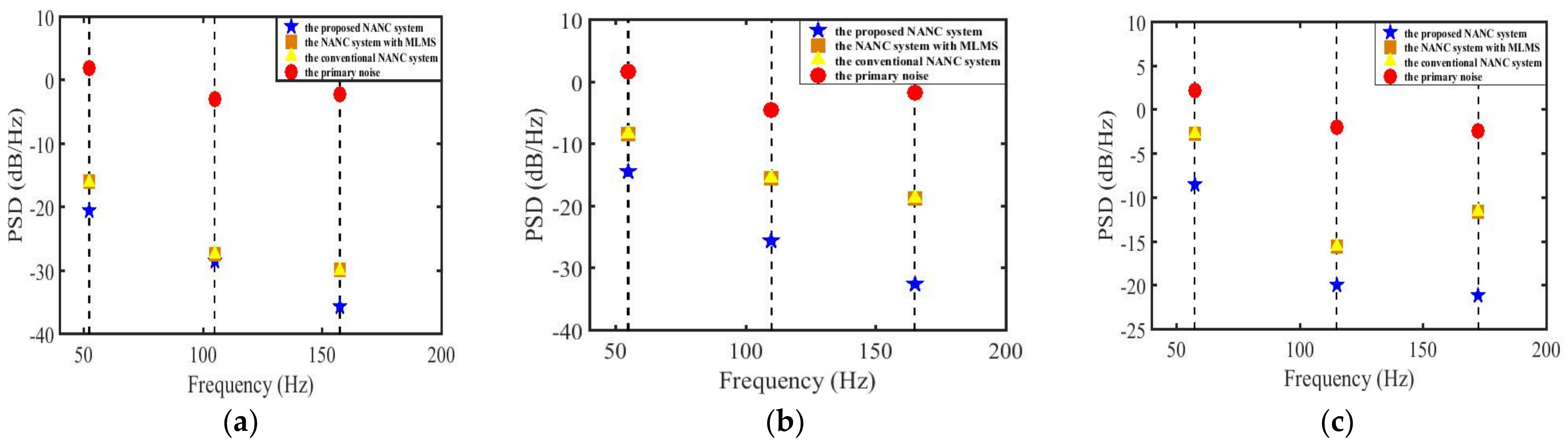
4.3. Simulation 3: Power Spectrum Density
The power spectrum density (PSD) of the primary noise and noises of three compared algorithms under different FM
Figure 11 shows the peaks of the PSDs at different frequencies in three algorithms. In the above pictures, the proposed NANC system has the lowest PSD among the three algorithms under different FMs. Clearly, it is capable for all three algorithms to eliminate the main tone in the primary noise. In Figure 11b, it can be seen the higher the frequency, the smaller the PSD of the error signal in the curve of the proposed NANC system, 5 dB, 10 dB, 13 dB, respectively, decreased compared with the other NANC systems. Similar results could be obtained in Figure 11c. Overall, the proposed NANC system has potential advantages over other frequency correction methods.
5. Conclusions
In this paper, a structure of a NANC system with the combination of frequency compensation and the LMP algorithm was proposed to accommodate large FM and uplink robustness. This method can not only accommodate a 15% FM, but also significantly improves the convergence rate, especially for a large FM. In addition, the tracking ability has been greatly improved for the sudden acceleration and deceleration. When a 10% FM occurs, the proposed system is drastically reduced from 7.5 s to 1.5 s when the system reaches the steady state. Even for a larger FM, with 15%, the proposed system converges in almost five seconds. It demonstrates the superior convergence rate of the proposed system when facing the FM caused by the sensors. Furthermore, the simulation results for the tracking capability demonstrate that the new frequency compensation performs better in handling the instability problem in the primary noise. Furthermore, the application of the proposed system will be conducted in our future work.
Author Contributions
Conceptualization, T.Y. and C.L.; methodology, T.Y.; formal analysis, T.Y.; project administration, C.L.; resources, C.L.; software, T.Y. and P.Y.; writing—original draft, T.Y.; writing—review and editing, P.Y., J.J. and J.W. All authors have read and agreed to the published version of the manuscript.
Funding
This research was funded by The National Key Research and Development Program of China (Grants No. 2017YFB0503500).
Institutional Review Board Statement
Not applicable.
Informed Consent Statement
Not applicable.
Data Availability Statement
All data in this paper are available from the corresponding author upon reasonable request. There are no additional data.
Conflicts of Interest
The authors declare no conflict of interest.
References
- Wang, X.; Bian, H.; Dong, Y.; Kang, N.; Hu, W. Risk assessment of noise-induced hearing loss among workers in railway transportation equipment manufacturing enterprises. Wei Sheng Yan Jiu J. Hyg. Res. 2022, 51, 904–910. [Google Scholar] [CrossRef]
- Mohd, S.M.A.; Zinnirah, W.; Kamaliana, K.N. Effects of Noise Hazards towards Physiology Especially Heart Rate Performance among Worker in Manufacturing Industry and Their Prevention Strategies: A Systematic Review. Iran. J. Public Health 2022, 51, 1706–1717. [Google Scholar] [CrossRef]
- Al-Harthy, N.A.; Abugad, H.; Zabeeri, N.; Alghamdi, A.A.; Al Yousif, G.F.; Magdy, A. Darwish. Noise Mapping, Prevalence and Risk Factors of Noise-Induced Hearing Loss among Workers at Muscat International Airport. Int. J. Environ. Res. Public Health 2022, 19, 7952. [Google Scholar] [CrossRef]
- Levak, K.; Horvat, M.; Domitrovic, H. Effects of noise on humans. In Proceedings of the 2008 50th International Symposium ELMAR, Borik Zadar, Croatia, 10–12 September 2008; pp. 333–336. [Google Scholar]
- Ho, C.Y.; Shyu, K.K.; Chang, C.Y.; Kuo, S.M. Efficient narrowband noise cancellation system using adaptive line enhancer. IEEE/ACM Trans. Audio Speech Lang. Process. 2020, 28, 1094–1103. [Google Scholar] [CrossRef]
- Pedro, R.L.; Raúl, M.F.; Fernando, A.M.; Guillermo, P.-N. An Alternative Approach to Obtain a New Gain in Step-Size of LMS Filters Dealing with Periodic Signals. Appl. Sci. 2021, 11, 5618. [Google Scholar]
- Wen, L.; Huang, B.; Pedro, R.L.; Raúl, M.F.; Fernando, A.M.; Guillermo, P.N. Modified Filtered-X Hierarchical LMS Algorithm with Sequential Partial Updates for Active Noise Control. Appl. Sci. 2020, 11, 344. [Google Scholar]
- Gan, W.S.; Mitra, S.; Kuo, S.M. Adaptive feedback active noise control headset: Implementation, evaluation and its extensions. IEEE Trans. Consum. Electron. 2005, 51, 975–982. [Google Scholar] [CrossRef]
- Ho, C.Y.; Shyu, K.K.; Chang, C.Y.; Kuo, S.M. Integrated active noise control for open-fit hearing aids with customized filter. Appl. Acoust. 2018, 137, 1–8. [Google Scholar] [CrossRef]
- Samarasinghe, P.N.; Zhang, W.; Abhayapala, T.D. Recent advances in active noise control inside automobile cabins: Toward quieter cars. IEEE Signal Process. Mag. 2016, 33, 61–73. [Google Scholar] [CrossRef]
- Elliott, S.J. A Review of Active Noise and Vibration Control in Road Vehicles; University of Southampton: Southampton, UK, 2008. [Google Scholar]
- Shoureshi, R.; Knurek, T. Automotive applications of a hybrid active noise and vibration control. IEEE Control Syst. Mag. 1996, 16, 72–78. [Google Scholar]
- Kim, H.-S.; Hong, J.-S.; Oh, J.-E. Active noise control with the active muffler in automotive exhaust systems. JSME Int. J. Ser. C Mech. Syst. Mach. Elem. Manuf. 1998, 41, 178–183. [Google Scholar]
- Lupo, F.C.; Jordan, C.; Mario, M. Investigation of an engine order noise cancellation system in a super sports car. Acta Acust. 2023, 7, 1. [Google Scholar] [CrossRef]
- Zhang, S.; Zhang, L.; Meng, D.; Pi, X. Active control of vehicle interior engine noise using a multi-channel delayed adaptive notch algorithm based on FxLMS structure. Mech. Syst. Signal Process. 2023, 186, 109831. [Google Scholar] [CrossRef]
- Cao, Y.; Deng, Z.; Zhang, Y.; Chen, D. Analysis and active control of low frequency booming noise in car. High Technol. Lett. 2015, 21, 414–421. [Google Scholar]
- Bagha, S.; Das, D.P.; Behera, S.K. An Efficient Narrowband Active Noise Control System for Accommodating Frequency Mismatch. IEEE/ACM Trans. Audio Speech Lang. Process. 2020, 28, 2084–2094. [Google Scholar] [CrossRef]
- Shi, D.; Gan, W.S.; Lam, B.; Wen, S. Feedforward Selective Fixed-Filter Active Noise Control: Algorithm and Implementation. IEEE/ACM Trans. Audio Speech Lang. Process. 2020, 28, 1479–1492. [Google Scholar] [CrossRef]
- Xiao, Y.; Ma, L.; Khorasani, K.; Ikuta, A.; Xu, L. A fILTERED-X RLS based narrowband active noise control system in the presence of frequency mismatch. In Proceedings of the IEEE International Symposium on Circuits and Systems, Kobe, Japan, 23–26 May 2005; pp. 260–263. [Google Scholar] [CrossRef]
- Jeon, H.J.; Kim, S.W.; Park, M.W.; Lee, W.G.; Chang, T.G.; Kuo, S.M. Frequency mismatch in narrowband active noise control. In Proceedings of the ICASSP, IEEE International Conference on Acoustics, Speech and Signal Processing, Dallas, TX, USA, 14–19 March 2010; pp. 345–348. [Google Scholar] [CrossRef]
- Kuo, S.; Morgan, D. Active Noise Control Systems: Algorithms and DSP Implementations; Wiley-Interscience: Hoboken, NJ, USA, 1996. [Google Scholar]
- Xiao, Y.; Ma, L.; Khorasani, K.; Ikuta, A. A new robust narrowband active noise control system in the presence of frequency mismatch. IEEE Trans. Audio Speech Lang. Process. 2006, 14, 2189–2200. [Google Scholar] [CrossRef]
- Liu, J.; Sun, J.; Xiao, Y. Mean-sense behavior of filtered-X LMS algorithm in the presence of frequency mismatch. In Proceedings of the ISPACS 2012—IEEE International Symposium on Intelligent Signal Processing and Communications Systems, Tamsui, Taiwan, 4–7 November 2012; pp. 374–379. [Google Scholar] [CrossRef]
- Xiao, Y.; Ikuta, A.; Ma, L.; Khorasani, K. Stochastic analysis of the FXLMS-based narrowband active noise control system. IEEE Trans. Audio Speech Lang. Process. 2008, 16, 1000–1014. [Google Scholar] [CrossRef]
- Kuo, S.M.; Nallabolu, S.P. Analysis and correction of frequency error in electronic mufflers using narrowband active noise control. In Proceedings of the 2007 IEEE International Conference on Control Applications, Singapore, 1–3 October 2007; pp. 1353–1358. [Google Scholar] [CrossRef]
- Sun, J.; Ma, F.; Huang, B.; Wen, L. A narrowband active noise control system with frequency mismatch compensation. In Proceedings of the 2014 Asia-Pacific Signal Information Processing Association Annual Summit and Conference APSIPA 2014, Siem Reap, Cambodia, 9–12 December 2014; Volume 19, pp. 990–1002. [Google Scholar] [CrossRef]
- Huang, B.Y.; Chang, L.; Ma, Y.P.; Sun, J.W.; Wei, G. A new narrowband ANC system against nonstationary frequency mismatch. Zidonghua Xuebao/Acta Autom. Sin. 2015, 41, 186–193. [Google Scholar] [CrossRef]
- Xia, G.-F. A Method for Accommodating Frequency Mismatch in Narrowband Active Noise Control. Master’s Thesis, Nanjing University of Aeronautics and Astronautics, Nanjing, China, 2016. [Google Scholar]
- Mao, M.-F.; Liu, J. Real-time Simulation for Methods of Accommodating Frequency Mismatch in Narrowband Active Noise Control. Sci. Technol. Eng. 2016, 16, 38–44. [Google Scholar]
- Shadaydeh, M.; Kawamata, M. Performance analysis of adaptive IIR notch filters based on least mean P-power error criterion. In Proceedings of the 2003 IEEE International Symposium on Circuits and Systems, Bangkok, Thailand, 25–28 May 2003; pp. 377–380. [Google Scholar] [CrossRef]
- Huang, B.; Sun, J.; Wei, G.; Xiao, Y. An active noise control system for the frequency mismatch problem in fan noise. In Proceedings of the ISPACS 2018—2018 International Symposium on Intelligent Signal Processing and Communication Systems, Ishigaki, Japan, 27–30 November 2018; pp. 264–267. [Google Scholar] [CrossRef]
- Kukde, R.; Manikandan, M.S.; Panda, G. Development of a novel narrowband active noise controller in presence of sensor error. In Proceedings of the 2014 International Conference on Advances in Computing, Communications and Informatics, ICACCI, Delhi, India, 24–27 September 2014; pp. 2735–2739. [Google Scholar] [CrossRef]
- Cheng, Y.; Li, C.; Chen, S.; Ge, P.; Cao, Y. Active control of impulsive noise based on a modified convex combination algorithm. Appl. Acoust. 2022, 186, 108438. [Google Scholar] [CrossRef]
Figure 1.
Block diagram of conventional FXLMS algorithm.
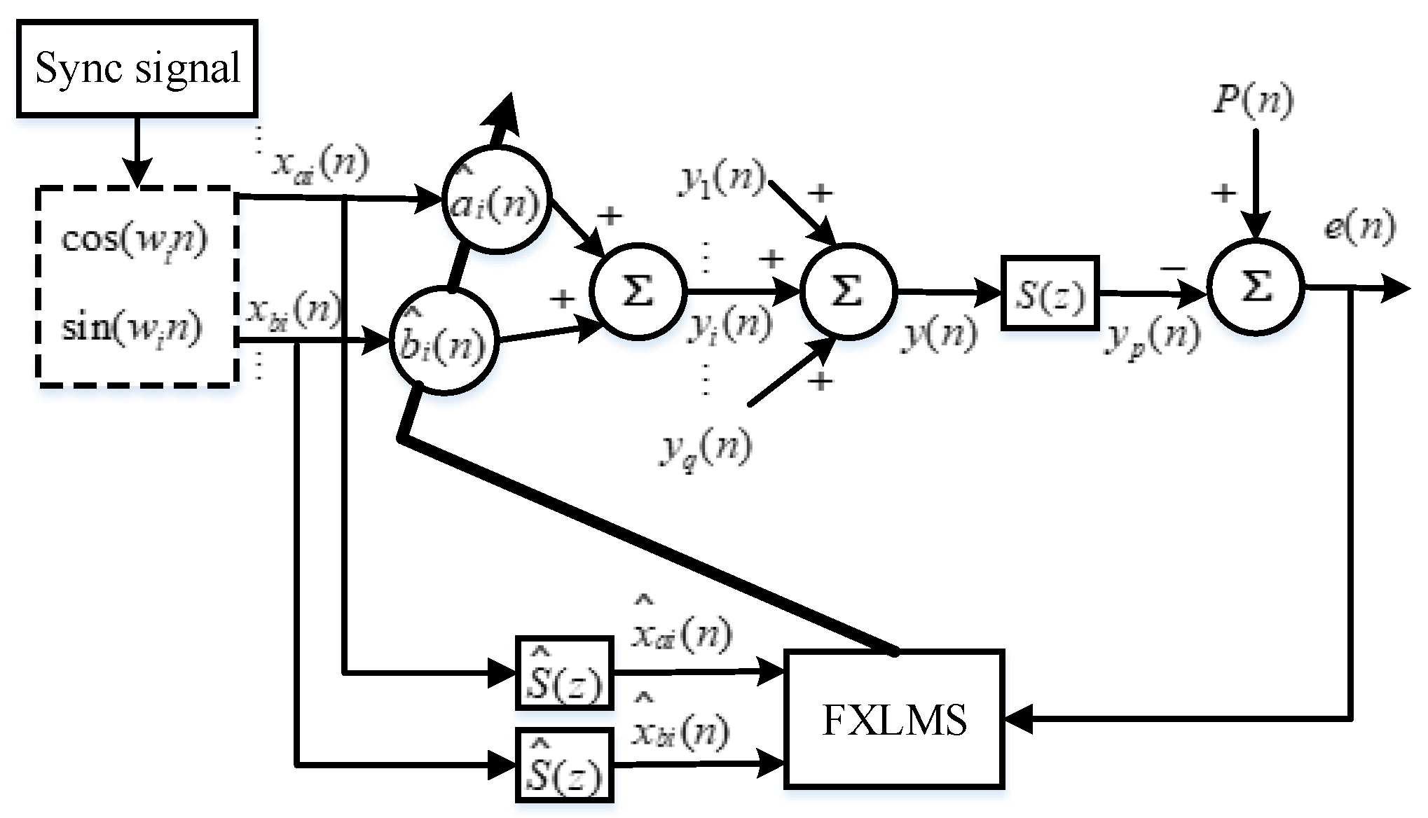
Figure 2.
Levels of residual noise signals for the conventional NANC system (true primary noise frequency:, reference signal frequency: , original amplitude:,, reference signal:, the step size: μ = 0.005, the secondary path: M = 11, ,, 40 runs, (a) Conventional NANC system (without FM). (b) Conventional NANC system (with 1% FM).
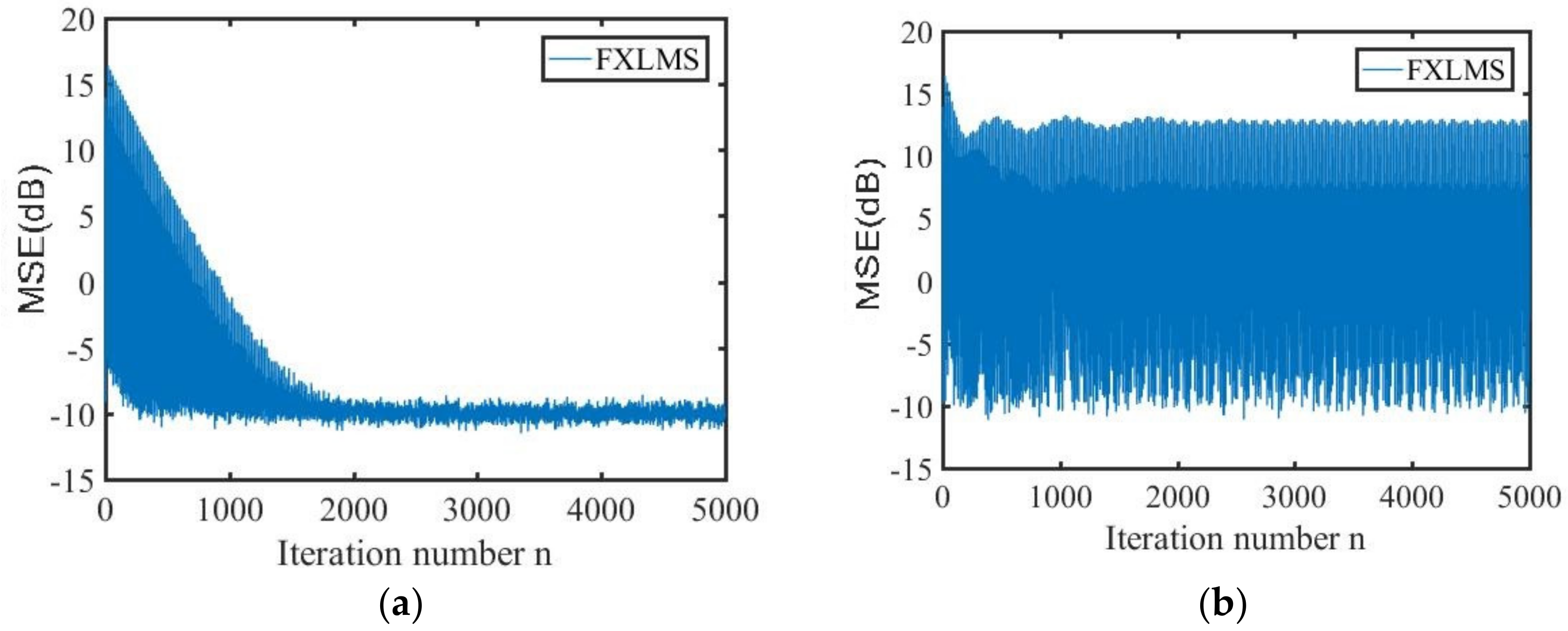
Figure 3.
The block of proposed NANC system.

Figure 4.
MSE of different k under different FM. (a) Without FM (b) Under 5%FM. (c) Under 10%FM (d) Under 15%FM.
Figure 4.
MSE of different k under different FM. (a) Without FM (b) Under 5%FM. (c) Under 10%FM (d) Under 15%FM.
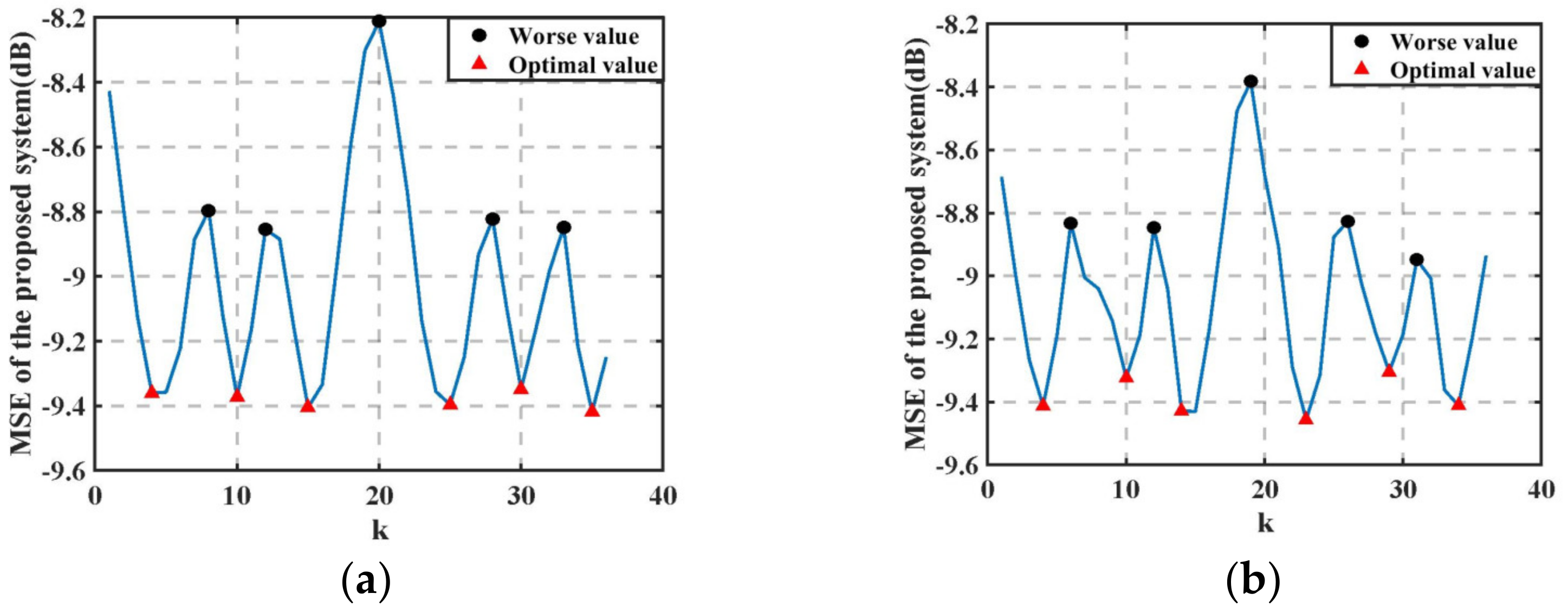

Figure 5.
Under 5%FM (a) the conventional NANC system (b) the system with MLMS (c)the proposed system.
Figure 5.
Under 5%FM (a) the conventional NANC system (b) the system with MLMS (c)the proposed system.

Figure 6.
Under 10%FM (a) conventional NANC system (b) the system with MLMS (c) proposed system.
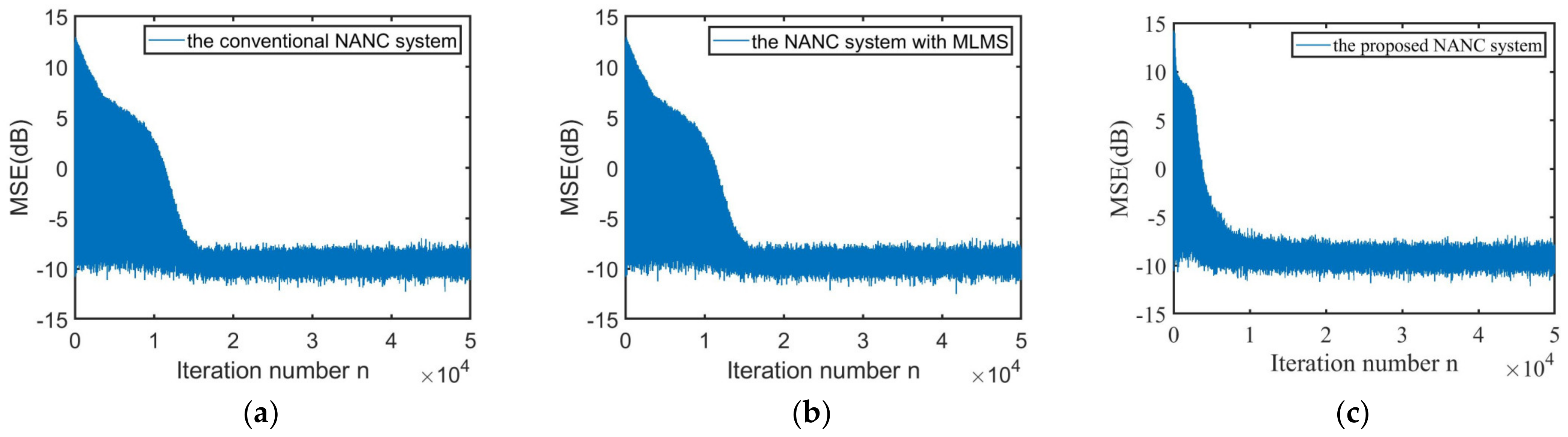
Figure 7.
Under 15%FM (a) the conventional NANC system (b) the system with MLMS (c) proposed system.
Figure 7.
Under 15%FM (a) the conventional NANC system (b) the system with MLMS (c) proposed system.
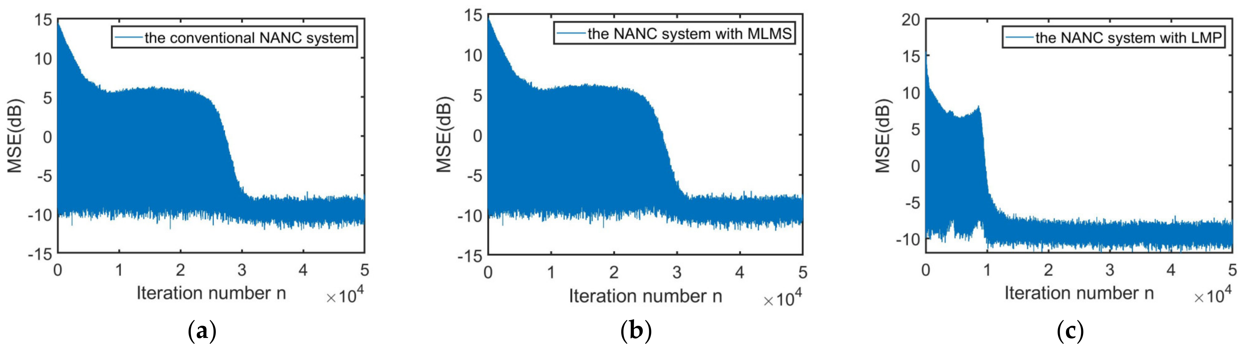
Figure 8.
Under 20% FM (a) the system with MLMS (b) the proposed system.

Figure 9.
MSE of AR-related coefficients performance for various methods under 15% FM.

Figure 10.
Tracking ability of the proposed algorithm versus its counterparts with different FM. (a) 5% FM. (b) 10% FM.
Figure 10.
Tracking ability of the proposed algorithm versus its counterparts with different FM. (a) 5% FM. (b) 10% FM.

Figure 11.
The peaks of PSDs of primary noise and residual noises of the three algorithms. (a) 5% FM. (b) 10% FM. (c) 15% FM.
Figure 11.
The peaks of PSDs of primary noise and residual noises of the three algorithms. (a) 5% FM. (b) 10% FM. (c) 15% FM.

Table 1.
The MSE with Different k under Different FMs(dB).
| Parameters | K = 8 | K = 14 | K = 20 | K = 32 |
|---|---|---|---|---|
| FM = 10% | −8.4999 | −9.43 | −9.012 | −9.424 |
| FM = 5% | −9.041 | −9.428 | −8.677 | −9.007 |
| Without FM | −8.796 | −9.159 | −8.212 | −8.972 |
Table 2.
The basic conditions.
| Parameters | Value |
|---|---|
| 1 kHz | |
| 0.1 | |
| FM C% (C is a random constant) | |
| S(z) |
Disclaimer/Publisher’s Note: The statements, opinions and data contained in all publications are solely those of the individual author(s) and contributor(s) and not of MDPI and/or the editor(s). MDPI and/or the editor(s) disclaim responsibility for any injury to people or property resulting from any ideas, methods, instructions or products referred to in the content. |
© 2023 by the authors. Licensee MDPI, Basel, Switzerland. This article is an open access article distributed under the terms and conditions of the Creative Commons Attribution (CC BY) license (https://creativecommons.org/licenses/by/4.0/).
Share and Cite
MDPI and ACS Style
Yao, T.; Li, C.; Yu, P.; Ji, J.; Wang, J. A New Effective Narrowband Active Noise Control System for Accommodating Frequency Mismatch. Appl. Sci. 2023, 13, 2416. https://doi.org/10.3390/app13042416
AMA Style
Yao T, Li C, Yu P, Ji J, Wang J. A New Effective Narrowband Active Noise Control System for Accommodating Frequency Mismatch. Applied Sciences. 2023; 13(4):2416. https://doi.org/10.3390/app13042416
Chicago/Turabian StyleYao, Tiannan, Chen Li, Ping Yu, Jiacheng Ji, and Jing Wang. 2023. "A New Effective Narrowband Active Noise Control System for Accommodating Frequency Mismatch" Applied Sciences 13, no. 4: 2416. https://doi.org/10.3390/app13042416
Note that from the first issue of 2016, this journal uses article numbers instead of page numbers. See further details here.