

Uncertainty of Estimated Rainflow Damage in Stationary Random Loadings and in Those Stationary per partes


1
Department of Mechanics, Biomechanics and Mechatronics, Faculty of Mechanical Engineering, Czech Technical University, Technická 4, 166 36 Prague, Czech Republic
2
Department of Engineering, University of Ferrara, Via Saragat 1, 44122 Ferrara, Italy
*
Authors to whom correspondence should be addressed.
Appl. Sci. 2023, 13(5), 2808; https://doi.org/10.3390/app13052808
Submission received: 30 January 2023
/
Revised: 17 February 2023
/
Accepted: 18 February 2023
/
Published: 22 February 2023
(This article belongs to the Special Issue Fatigue and Fracture Mechanics: Applications and Trends II)
Abstract
:The uncertainty of rainflow fatigue damage is evaluated for stationary loadings and for non-stationary switching loadings with a finite number of stationary states. The approach is based on confidence intervals constructed after direct analysis of stress-time histories. The accuracy of confidence intervals is verified first by numerical simulations, and then by experimental data measured in a mountain bike traveling under various driving and road surface conditions, yielding stationary and non-stationary switching loadings. Stationarity and non-stationarity of loading records is checked by a statistical method (run test). In experiments, a small set of records (validation set) is also collected and used to approximate the expected damage, which serves for verification purposes. Not only do numerical and experimental results confirm the correctness of the proposed confidence interval for damage, but they also emphasize its usefulness in real engineering applications.
1. Introduction
The great majority of structural details are subjected, in service, to irregular or random loadings. It is easy to find examples in a variety of engineering fields: oceanic (offshore structures and ships exposed to wave loadings) [1], aeronautics and aerospace (airplanes during a flight) [2], automotive (cars subjected to road-induced loadings) [3,4]. With such random loadings, the structural integrity assessment is based on the fatigue damage computed on a stress-time history by rainflow counting and the Palmgren–Miner rule [5].
Often, one or more stress-time histories of finite length are available from measurements. It is unlikely that such histories, no matter how long, can include all the possible fatigue cycles to which the structural detail will be subjected in its entire service life. Certain stress cycles may not be observed in a short duration measurement. Fatigue cycles have in general different amplitudes and mean values, which in turn yield different values of damage for each stress-time history. Stated another way, the fatigue damage of a random stress-time history of length is a random variable following a certain probability distribution with expected value and variance . Expected value and variance represent averages over an infinite population of damage values computed from an infinite ensemble of records—clearly, an abstraction impossible to be obtained in practice.
Based on this matter of facts, the following question naturally arises: what conclusions can confidently be drawn from the knowledge of the damage computed from a few stress-time histories of finite length, or even from only one? This issue is intimately related to the statistical uncertainty of the observed damage values.
The problem has been tackled by different approaches in the literature. Since the 1960s, some authors developed analytical formulae that allowed the expected value and variance of damage—or equivalently the coefficient of variation (CoV) —to be determined from several statistical properties of the random record, or from its power spectral density function. These approaches are restricted to certain load models (linear oscillator) [6,7,8,9] or to loadings with specific types of power spectral density (narrowband [10,11], multimodal [12] or wide band [13]). Extension to non-Gaussian loadings has also been proposed recently [14]. Interesting is the method presented in [15] in which the CoV of damage is estimated from only one sample record.
The uncertainty in fatigue damage—and its correlation with various sources of randomness—has been investigated, in more recent articles, in a probabilistic and/or reliability framework based on different modeling strategies (e.g., machine learning algorithm [16], surrogate model [17]) and methods (e.g., piecewise stochastic rainflow counting [18], Bootstrap error circle [19]), with applications and case studies spanning various engineering fields (e.g., maritime [20,21], structural [22], automotive [23,24]).
Differently from the previous methods, an approach—also devised in [13]—used confidence intervals to evaluate the uncertainty of rainflow damage, and specifically to enclose the expected damage when only few stationary stress-times histories, or only one, are available. Although in [13] the approach was positively benchmarked against numerical simulation results, it is only applicable to stationary loadings with time-invariant statistical properties. This characteristic may not fully represent the actual loading conditions in certain structural details, in which random loadings have statistical properties that change over time and, therefore, are non-stationary.
Among the broader class of non-stationary loadings, in many engineering applications, the non-stationary loadings are formed by a sequence of stationary states—they are called switching loadings. Examples could be offshore structures and ships exposed to a sequence of stationary sea states; airplanes during the sequence of taxiing, taking off, cruising, maneuvering and landing; wind turbines under wind loadings caused by weather conditions; and cars and bikes subjected to different road surfaces and velocities. Evaluating the uncertainty of rainflow damage for such types of switching loadings has therefore a great practical relevance.
Starting from this premise, this paper aims to extend the confidence interval of damage for stationary loadings to the case of non-stationary loadings of the switching type. The obtained solution is benchmarked against numerically simulated and measured non-stationary loadings, the latter being recorded in a mountain bike traveling in different riding conditions and over various tracks.
The paper is organized as follows: after a brief theoretical background (Section 2), the confidence interval for the stationary case is first reviewed (Section 3) and then extended to the case of switching loadings (Section 4). The confidence interval for the non-stationary case is checked by simulated loadings (Section 5), whereas measured loadings are used to validate the solutions for both stationary and non-stationary cases (Section 6).
2. Expected Fatigue Damage for a Random Loading
Let , , be a time-varying signal as measured at a critical point in a structure, whether the signal is load, stress or strain. Throughout the paper, it will be referred to as a stress-time history (or stress record). The fatigue damage of under the Palmgren–Miner linear rule is [5]
where is the number of cycles to failure at stress amplitude and is the number of rainflow cycles counted in . Equation (1) is very general as it applies to both stationary and non-stationary loadings, and to any S–N equation. Often, constant amplitude experimental data are best-fitted by a S–N curve , where is the fatigue strength coefficient and the inverse slope.
Damage depends on the stress-time history of duration from which it was computed. It has a statistical uncertainty coming from two sources: load (e.g., stress amplitudes , number of counted cycles ) and material strength (coefficient and inverse slope ). The latter can be taken into account by means of a characteristic S–N line defined for a low probability of failure (e.g., 2.3% or less) [25,26]. The focus of this paper is therefore on the randomness of the load, which is reflected into the randomness of and . Because of this, damage is a random variable following a certain probability distribution with expected value and variance .
Intuitively, can be thought as an average over an infinite population of damage values, which are computed from an infinite number of load records. This situation is purely theoretical. In real engineering applications, the common situation is indeed that in which only few stress-time histories (if not even only one) with finite time duration are available from measurements. In this case, E[D(T)] remains unknown. A statistical method is needed to draw conclusions on based on .
3. Confidence Interval of Damage: Stationary Case
This section describes how to construct the confidence interval on when is computed from (i) multiple (two or more) records (Case M) or (ii) a single record (Case S).
3.1. Case M: Multiple Stress-Time Histories
Assume that stress-time histories , of same duration are available, e.g., from measurements replicated under the same conditions. The damage values , of each are characterized by the sample mean and sample variance [27]:
These sample estimates represent the unbiased estimators of the (unknown) expected value and variance of the damage , respectively. In the hypothesis of normally distributed damage, the above sample values allow the confidence interval on the expected damage (with variance unknown) to be constructed as [27]
in which is the upper percentage point of t distribution with degrees of freedom. For large (for example, ), the t distribution approaches a standard normal distribution, . In Equation (3), the only unknown is .
Predictably, the confidence interval becomes increasingly narrower if increases. If the number of load records were infinite, no statistical uncertainty would be present; would be equal to , and the confidence interval would have a zero width (zero prediction error).
Equation (3) relies on the hypothesis of normally distributed damage , which can be assumed under the validity of the central limit theorem in the limit . Under this hypothesis, the Palmgren–Miner damage is, in fact, the sum of a countless number of damage values from individual cycles. The hypothesis of central limit theorem has been supported by many authors [6,7,8,9,28]. In [11], it was concluded that the departure from the normal distribution for the damage is only marginal, especially for low values of the CoV of damage, which in turn indicates that in practical situations, is usually long enough for the central limit theorem to apply. Recent studies [29] have nevertheless discovered that, for larger values of both CoV and S–N slope (i.e., less steep S–N line), the damage distribution tends to be skewed and non-normal, even though this conclusion has been drawn based on a very small number of cycles (3200) that, while used for accentuating the skewness of damage distribution, seem unrealistically too small for common engineering applications. Even in the case (discussed in Section 3.2) of block subdivision, which yields a block length , the number of blocks is small so that remains long enough to assume that is normally distributed.
3.2. Case S: Single Stress-Time History
This is the most common and interesting case in which only a single stress-time history of duration is available, e.g., from only one measurement. In order to construct the confidence interval on as in Case M, a sample of damage values needs to be obtained first. To this end, in a preliminary stage, is divided into disjoint blocks of equal time length . The damage of blocks is , .
It is worth emphasizing that since the entire record is stationary and its subdividing blocks fully disjoint (not overlapped), the rainflow cycles counted in each block form independent sets, and their amplitudes have the same statistical distribution. As a result, the block damages , are independent and identically distributed random variables, with a common value of variance and zero covariance, (). The damage of the undivided record is
where denotes the sample mean of block damage:
while is the sample variance of block damage, to be used shortly.
The sign in the previous equation signposts a small approximation. In fact, the block subdivision determines a small fraction of rainflow cycles to be lost, namely, those cycles formed by peaks and valleys falling in distinct blocks after subdivision. While these cycles would be counted in the undivided record , after subdivision they are not counted anymore. Compared to the number of cycles in each block, the amount of lost cycles is negligible if the block length is sufficiently long. This condition on , in turn, implies that the number of blocks cannot increase indefinitely. As a rule of thumb, the minimum value for must assure a minimum of cycles in each block; this condition ensures that the approximation in Equation (4) is perfectly acceptable [13].
As for Case M, the sample values in Equation (5) allow the confidence interval on (for a single block) to be constructed as [27]
Here, is the upper percentage point of the t distribution with degrees of freedom; for , it is .
The confidence interval in Equation (6) can be further elaborated. As an intermediate step, take the expected value and variance of Equation (4):
where is the variance of block damage—note that, likewise the expected damage , also the variances and refer to an infinite population of damage values and then are unknown. In both formulae in Equation (7), the second equal sign takes advantage of the fact, already mentioned above, that the random variables are independent and identically distributed, which implies that and for any , and that for .
After multiplying Equation (6) by :
and substituting the results of Equations (4) and (7), the final expression is
where the unknown variance of damage is approximated by the sample variance of block damage as [13].
Equation (9) is the confidence interval on the (unknown) expected damage . Other quantities can easily be computed: is the damage of the whole stress-time history , is the sample standard deviation of derived from the sample standard deviation of block damage, is tabulated.
4. Confidence Interval of Damage: Non-Stationary Case
This section extends the result of Section 3.2—which has much greater practical relevance—to the case of a non-stationary loading of switching type, formed by a sequence of stationary states. As a preparatory result, the confidence interval on the sum of expected values of independent and normally distributed random variables is developed.
4.1. Confidence Interval on the Sum of Independent Normal Random Variables
The following results follow the same reasoning used for the confidence interval on the difference in expected values [27,30]. As a starting point, and with the purpose of illustrating the approach, it is useful to discuss first the simplest case of the sum of two independent and normally distributed random variables and with expected values , and variances , .
The goal is to construct a confidence interval on in the hypothesis of different and unknown variances , . Inference will be based on two random samples of size and from and , denoted as , and , .
Under the previous hypotheses on ’s, it follows that is normally distributed with expected value and variance [27]. A logical point estimator of is the sum of sample means , each one defined as . It is well known that each is normally distributed with expected value and variance [27]. Since the sample means and of independent random variables are also independent, the estimator has expected value and variance .
In order to derive a confidence interval on , and taking advantage of the above findings, it is useful to consider the statistic:
which has approximately a t distribution with degrees of freedom [27,30]:
If not integer, has to be rounded down to the nearest integer [27]. In previous expressions, is the sample variance of the i-th sample , where . Note that symbol in Equation (11) denotes the numerical value of computed from an observed sample of values ; as usual in statistics, lowercase letters indicate observed values of random variables or estimators, indicated by uppercase letters.
From the distribution of and the probability statement , it is possible to construct the approximate confidence interval on the sum of expected values as
where is the upper percentage point of the t distribution with degrees of freedom given in Equation (11). Symbols , and , indicate the numerical values, respectively, of the sample mean and sample variance calculated from the two observed samples of and (by definition, the sample mean is ).
It is now straightforward to generalize the result in Equation (12) to the case of a random variable sum of independent and normally distributed random variables with expected values and unequal variances . In this case, the approximate confidence interval on the sum is
where and denote the sample mean and sample variance of the i-th random sample , with observations for the random variable ; is the upper percentage point of the t distribution with the following number of degrees of freedom:
As before, a fractional value of must be rounded down to the nearest integer [27]. In the case, analyzed in Section 4.2, of equal sample sizes (for any ), the previous expression simplifies as .
The level of accuracy of the approximate confidence interval in Equation (13) was checked by numerical simulations in which various sets with different numbers of random variables , each with different expected value and variance , were examined. The selected values of and allowed for a total of sixteen possible combinations for the random variables . The first six are listed in Table 1.
Not all random variables ’s were considered simultaneously; rather, their number was made to vary as , i.e., from only two variables up to all sixteen variables included. Once has been selected, a random sample of size was generated from the normal distribution of each with parameters and . Different sample sizes in the range were considered.
For each combination of and , the random sampling yielded samples of size , the values of which were used to construct the 95% confidence interval as per Equation (13). This confidence interval, by definition, may or may not enclose the expected value . If the procedure is repeatedly applied, it is expected that 95% of confidence intervals will enclose . To verify this assertion, the random sampling and construction of the confidence interval (for given combinations of and ) were repeated times; in this large set, the fraction of confidence intervals enclosing represented the estimated confidence level to be compared with the theoretical value 95%.
The outcome for a few selected combinations of , which are in fact well representative of a general trend, is summarized in Table 2. It is observed that, for and being both very small, Equation (13) gives confidence levels larger than the theoretical value 95%; for greater values of and , the difference almost disappears. Only for the lowest values of , the difference may occasionally be large, for example, reaching 98.59% when and . Nevertheless, this smallest sample size is only included here for comparative purposes; it being usually not used in practice. Apart from this value, for larger values of , the estimated confidence level converges to the theoretical value, for any . This outcome confirms the accuracy of the approximated confidence interval in Equation (13).
4.2. Confidence Interval of Damage for a Switching Loading with Two or More States
Thanks to Equation (13), the results of Section 3.2 are now extended to a non-stationary stress-time history of duration that switches between a finite number of stationary states—an example with three states (1, 2, 3) is depicted in Figure 1.
Compared to the stationary case, the procedure now requires an additional step in which the distinct stationary states in are first identified. This identification can be performed by checking for abrupt changes, for example, in the root-mean-square (rms) value in , as it will be demonstrated in Section 6.
Since each stationary state represents a portion of the whole record , the total time length of sums the length of individual states as . In a similar way, the total damage of is the summation of the damage of individual loading states as [31]. The approximation sign in this equality is due to the fatigue cycles lost when separating the entire stress-time history into stationary segments and omitting the transitions cycles between them (an example is the range between the global maximum and global minimum if they do not occur within the same segment—typical for the ground–air–ground cycle in the aviation industry). On the other hand, since the number of segments or stationary states is generally small, the amount of these lost cycles—and the damage they contribute—is negligible compared to that of the multitude of other cycles counted within individual states.
Assume that in the non-stationary stress-time history , a total of distinct stationary states with lengths , have been identified. As in the stationary case, each state is further subdivided into blocks of length , see Figure 1. Since distinct states have different lengths but share a common , block lengths in every state are in general different , . It is noted that the choice of a common for all states is not strictly necessary, though it simplifies the following theoretical solution.
State identification and block subdivision give the damage values , with (state index) and (block index). Damage refers to block in state . Note that , represent a sample of observed values for the random variable (block damage of state ), with expected value .
By following the procedure of Section 3.2, the values are used to compute the sample mean and sample variance of block damage in state :
which are computed for from 1 to , so there are in total values of and . There are also values of , .
At this stage, the goal is to construct a confidence interval on the sum of expected block damages, namely . The similitude with the problem explained in Section 4.1 is now apparent, provided that the quantities , and in Equation (13) are replaced by , and , respectively. The number of random variables coincides with the number of states, ; the sample size is the number of blocks, . The confidence interval on the sum of expected block damages then is
where is the usual upper percentage point of a t distribution with degrees of freedom (case of common for any ):
Equation (16) can be further elaborated to a simpler form for practical use. After substituting in Equation (16) the sample mean in Equation (15) and then multiplying by , the confidence interval expression becomes
If Equation (7) is now considered, it is easy to recognize that represents the expected damage for the -th state. Furthermore, the single summation gives the expected damage of the entire non-stationary record . The double summation corresponds to the total damage of —the approximation in the equal sign lies in the small amount of cycles lost after block subdivision, already discussed in previous sections.
Upon substituting the quantities obtained so far, and , it is possible to rewrite Equation (18) into the final expression of the confidence interval on for a single non-stationary switching stress-time history :
In this formula, the quantities and are known: is the fatigue damage of the entire switching stress-time history , is the sample standard deviation of the block damage for the -th stationary state. The expected damage is unknown.
A minimum number of segments is required. Similarly, the number of blocks should be to allow the sample values of each stationary state to be computed. Interesting is to note that in the limit case (the switching loading has only one stationary state), Equation (19) converges to Equation (9), whereas Equation (17) simplifies into , which is indeed the solution for the stationary case.
It is finally worth emphasizing an important remark on the ordering of stationary states in the switching loading . The simplified situation depicted in Figure 1, in which states follow one another in their full length, is in fact not required. More realistically, and as also observed in practical applications [32], the same stationary state may appear randomly and repeatedly in .
In order to apply the approach described so far, it is irrelevant in which time sequence the states come in succession and how many times the same state appears in initially, provided that there are limited differences in mean values between states. If one or more states appear more than once in different time sectors of , it is necessary to reorder them: sectors belonging to the same state are shifted to adjacent positions so that each state appears only once in its full length. An illustrative example is shown in Figure 2. It shows three states split into sectors of different length. After reordering, sectors 1a and 1b from the same state 1 are joined to form one single portion 1a + 1b of duration . The same reordering joints the sequence 2a + 2b and 3a + 3b. The confidence interval on expected damage in Equation (19) is to be applied to the reordered stress-time history.
5. Verification by Simulated Switching Loadings
5.1. Simulation of Load Cases
The stationary case has already been checked in [13]. Therefore, attention here is focused on the switching case. Three types of switching loadings, which may represent practical cases, are considered:
- Load B: same and as Load A but with different lengths with values: s (state 1), (state 2), s (state 3);
- Load C: sequence of four states arranged in a random sequence. Since states 1 and 2 appear twice (see Figure 4a), the analysis requires a state reordering (the reordered sequence, with full state lengths , is shown in Figure 4b). States have the following characteristics: s, , (state 1); , , (state 2); s, and (state 3); s, , (state 4).
Each switching load is obtained by first simulating a sample loading separately for each stationary state and then by arranging the simulated loadings in the desired order.
The previous simulation procedure was repeated so that a total of realizations , were simulated for each load type A, B, C. This sample size is comparable to similar studies [11]. Fatigue damage values , were calculated for all realizations by assuming an S–N slope . A sample mean damage is computed as in Equation (2); since is very large, the approximation holds true with enough accuracy.
Besides the sample of large size , a smaller set of realizations—called the validation set—is also generated for each load type A, B, C. This validation set will become fundamental with measured loadings, see Section 6. In fact, whereas it is effortless to numerically simulate large samples of load realizations to be used for approximating accurately as above, it is instead almost impossible to collect a huge number of measured records, and the “small” validation set then becomes the only means to approximate . On the other hand, when the sample size reduces, it may be presumed that can occasionally be less close to because of the increased sampling variability. Introducing the validation set also in numerical simulations has the purpose to assess the accuracy of the approximation when is computed over a much smaller sample ().
The damage values , from the validation set are used to compute a sample mean and sample variance:
Obtained results show that the approximation has only a 2% difference lower than the approximation in which the sample mean damage is computed on the larger set . This confirms how a validation set of smaller size yields sufficiently accurate statistics, at least for the simulated realizations considered in this study.
As the last step in the simulation procedure, one additional switching load realization was generated for Load A, B, C and then used to construct the 95% confidence interval on according to the procedure of Section 4.2; the number of blocks ranged from 2 to 10. The results are presented in the next subsection.
5.2. Simulation Results
Figure 5a displays, for Load A, the confidence intervals (normalized to the expected damage) as a function of . Very similar trends (not shown) are obtained for Load B and Load C. For any , (approximated by ) always falls within the confidence interval. As increases, the interval width diminishes towards a sort of asymptote; this confirms that the prediction error cannot be decreased by subdividing the load states into infinitely many blocks. In fact, block subdivision does not add “new information”, such as new fatigue cycles, to the original undivided load.
The outcome in Figure 5a, though very promising, only represents one observation, and it cannot be used to draw general conclusions on the correctness of the method. In fact, a confidence interval, by definition, may or may not enclose the expected value ; a set of 20 confidence intervals (for the case ) is displayed in Figure 5b to show an example in which is not enclosed by the confidence interval.
If the construction of the 95% confidence interval described so far is repeated in a series of independent analyses, in the long run it is expected that 95% of the computed confidence intervals will enclose . To prove this statement, it is necessary to repeat the above procedure a multitude of times, and then count how often the confidence interval encloses —theoretically, it should be 95 out of 100 times. While the validation set is kept unchanged, switching loads are iteratively simulated times, and for each iteration, the confidence interval is constructed. The fraction of confidence intervals enclosing represents the estimated confidence level . As an example, for , the obtained values are 94.9% (Load A), 95.6% (Load B) and 95.2% (Load C), which are almost coincident with the theoretical value of 95%. Only in the limit case , the estimated confidence becomes larger (e.g., 98.1% for Load C), but it rapidly reduces as increases; it is then recommended to divide the stationary states into as many blocks as possible, compatibly with a minimum number of cycles in each block. In summary, simulations results have confirmed the accuracy of the proposed approach.
6. Verification by Loadings Measured in a Mountain Bike
6.1. Methods and Data Acquisition
The stress-time histories measured on the mountain bike are aimed at verifying the correctness of confidence intervals. The mountain bike (see Figure 6) has a frame of 6061 aluminum alloy, and a front fork of steel [31]. Two Rigida Cyber 10 size 700C wheels are coupled with 700 × 37c S207 semi-slick tires. The bicycle was equipped with an on-board data acquisition system capable to measure and store the strain-time histories during the bike ride. The on-board system is formed by a data acquisition system (mounted on the inclined tube of the bicycle frame), rechargeable battery (allocated on a support behind the seat), speedometer (with a sensor and a magnet fixed on a spoke) and two half-bridge strain gages (glued onto the fork). The strain gages, placed symmetrically around the left fork tube, are aligned in the longitudinal plane so as to measure the axial strains corresponding to the bending moment in the fork. The sampling frequency was 1000 Hz. After data acquisition, measured strain signals were converted into stress signals as , where is the elastic modulus of steel. When fully equipped, the mountain bike plus rider weighed about 77.2 kg. More details on the bicycle and on-board system can be found in [31].
Two types of circular off-road tracks were chosen for measurements. The tracks were plane (or almost plane) and made of different road surfaces. Track types and riding conditions were selected so that the measured records were (i) stationary or (ii) non-stationary of switching type. In the stationary case, the mountain bike moved at the approximately constant speed of 15 km/h over the same road made of gravel, see Figure 7a. In the non-stationary case, the bike moved over surfaces of different characteristics such as asphalt, gravel and grass, see Figure 7b, and with a speed varying from 10 to 20 km/h. In both stationary and non-stationary cases, the mountain bike was ridden by a rider of 65 kg, who remained seated for the entire duration of each measurement.
It has to be emphasized that the choice of these riding conditions—which are in fact not typical of a mountain bike in off-road use—was primarily dictated by the need to obtain stress-time histories that were stationary or non-stationary of switching type, which are the requirements for applying the confidence intervals. For the same reason, the measured records are not used here for evaluating the structural safety of the bicycle.
All measurements, carried out over fourteen consecutive days, gathered an amount of 41 stationary and 21 non-stationary load records, grouped as follows:
- 10 stationary records used as input for Case M in Section 3.1.
- 1 stationary record used as input for Case S in Section 3.2.
- 30 stationary records to form the validation set for the stationary case.
- 1 non-stationary switching record to be analyzed as in Section 4.2.
- 20 non-stationary switching records for the validation set of the non-stationary case.
All measured records are available in the section “Supplementary Materials”.
The two validation sets were used to compute a sample mean damage (validation damage) with which to approximate the expected damage as . Indeed, cannot be measured exactly as it refers to an infinite collection of load records. It is not superfluous to emphasize that the validation damage is only used here for verification purposes, that is, to verify whether the confidence intervals enclose the expected damage. The validation sets are not required in real practical situations.
Once measured, all stress-time histories (stationary and non-stationary) were scaled so that all data points from 0 to had a zero mean and unit variance. This scaling is perfectly acceptable as the stress-time histories are not used here for a structural integrity assessment of the bicycle; on the other hand, the scaling does by no means undermine the validity of the conclusions presented hereafter.
Figure 8 depicts two examples of stationary and non-stationary records after normalization. It is possible to appreciate, at least visually, how the non-stationary record does show significant variations over time of its mean and, more markedly, its variance, whereas the stationary record does not.
6.2. Detecting Stationarity/Non-Stationarity by the Run Test
The Wald–Wolfowitz run test (or simply run test) is a non-parametric hypothesis test to check whether a load record is stationary or non-stationary. Admittedly, in its original formulation (two sample version [33,34,35]), the run test was proposed as a hypothesis testing to verify whether two random variables X and Y follow the same probability distribution function. The acceptance or rejection of the hypothesis is based on the statistical distribution of “runs”. A “run” is a sequence of values from the same random variable (or ) that is preceded or followed by values from the other variable (or ), or by no observation at all—the ’s and ’s are values randomly sampled from X and Y and then pooled together to form a single bigger sample.
With a slight modification, the run test can also be used to test whether a single discrete sequence of values is truly random or contains an underlying deterministic trend. In this version, the application of the run test requires that a reference value (usually the median of the sequence of values) is introduced [35]. The median allows the initial sequence to be divided into two dichotomic categories: values above () and values below () the median. The original sequence of discrete values is then converted into a sequence (e.g., ) of two mutually exclusive sets, exactly as in the original version with two variables and . The “runs” are finally identified and counted; for example, the sequence has six runs marked with round brackets. Based on the definition of median, each category or counts an equal number of items () if, in the original sequence, the number of elements is even; if the number of elements is odd, the value equaling the median is ignored.
A further modification is finally required if the run test is to be applied to a random signal with continuous time values (here, “continuous” disregards the discrete time sampling always present in digitalized signals). The modification has the purpose of converting the signal into a set of discrete sequences of values. It consists in dividing the signal into a number, say, of consecutive but disjoint segments; then, for the signal portion within each segment, a statistical parameter—usually the signal root-mean-square (rms) value—is determined. This signal processing returns a discrete sequence of rms values , for which the median is then computed. This allows the ’s to be divided into values above () and below () the median. A discrete sequence of and is again obtained, for which the “runs” are identified and counted.
The number of runs, say , is a random variable because it depends on the observed sequence of and and, in turn, on the signal analyzed. Let be the number of values above/below the median. If this number is large (>10), the distribution of approaches a normal distribution with mean value and variance [33,35]:
The acceptance region for the null hypothesis “the sequence of ’s is truly random”, with a level of significance , is given by the inequality:
where and are tabulated [36], or they can be approximated (if ) by taking for a normal distribution with parameters , in Equation (22) [37].
Based on the value of (i.e., the number of runs in the sequence of rms values in ), conclusions can be drawn on the nature of . If falls inside the acceptance region as in Equation (22), the sequence of is presumed to be truly random, and accordingly, is classified as stationary. Conversely, if falls outside, is classified as non-stationary.
An important parameter in the run test is the number of segments, as it directly determines the segment time length . The important role of has been emphasized in [38]. In that study, it was discovered—though only empirically—that too long a value of has the effect of smoothing local variations in the rms value, if present, up to the point of hiding the presence of underlying trends. This effect can be understood quite intuitively by considering that the rms value of each segment, , is computed as a time average of the signal in that segment. It is then presumed that the value fully represents the signal rms value in that segment, regardless of whether the actual rms value is in fact constant within the segment. Any local fluctuation of the rms value within each segment is averaged out, indeed. As a direct consequence, the longer the segment length, the greater the averaging effect in each segment, with the risk of smoothing or even hiding any non-stationary fluctuation—the run test may classify the signal as stationary though it is not. Conversely, too short a segment length, while increasing the sensitivity to local temporal variations, tends also to enhance the presence of irregular fluctuations of rms values across adjacent segments that, being only due to a sampling variability, may erroneously indicate a false non-stationarity. Regrettably, the interesting observations made in [38] are not used to suggest practical recommendations for the optimal choice of .
For this reason, the run test is here applied by choosing two different values: and . Figure 9 illustrates the run test applied to one of the measured records belonging to the presumed “stationary” set. When , there are observations above and below the median; from statistical tables, the upper and lower limits in Equation (22) are and ; for a 5% significance level, . Since the observed number of runs is , and it falls within the acceptance region of the test (, the load record is classified as stationary.
The same conclusion is also confirmed by choosing a shorter window length, for which in general the verdict of the run test tends to be in favor of non-stationarity. For a window length , there are observations above and below the median, while the observed number of runs is , which again falls within the acceptance region defined, for 5% significance, as a function of . The load record is again classified as stationary. When applied to all other records of the “stationary” set, the run test (with both window lengths) classified them as being truly stationary.
When the run test is applied, instead, to the set of switching measured loading, the outcome is opposite. For the case of (see Figure 10a), the observed number of runs falls outside the acceptance region defined by the same number of observations as above. The stress-time history is classified as non-stationary. Nothing changes if the window length increases to , see Figure 10b. With a longer window length, the number of runs decreases to and again falls outside the acceptance region defined by the same observations as above. The same outcome “non-stationary” was obtained for all measured switching records.
6.3. Experimental Verification of Confidence Intervals: Stationary Case
In this section, the confidence intervals in Equation (3) (Case M) and (9) (Case S) are applied to the measured stationary records. In Case M, the analysis considered groups of records (with ranging from 2 to 10) selected from the 10 measured initially; in every group, each of the 10 records appeared only once. The records have damages , , used in Equation (2). In Case S, the individual record was subdivided into disjoint blocks (with ranging from 2 to 10). The block damages , are used in Equations (5) and (9). Finally, the validation set is used to approximate the expected damage as , where is computed by Equation (20) with from measured records in the validation set. Equation (20) also provides the sample variance of validation damage, . Damage computation considered an S–N slope .
The main statistics are summarized in Table 3. The first three columns (Case M) list the sample mean and sample standard deviation of damage as a function of . The last three columns (Case S) list the total damage calculated as and the standard deviation as , as a function of . Damage values are normalized to , standard deviations to .
In Case M, the sample mean damage varies with but not significantly. Apart from two exceptions, the trend of is to decrease as increases, the lowest value being for the largest sample of records (). In Case S, this trend is not observed, and remains almost independent of . Interestingly, at the largest , is about 50% greater than its value for in Case M. Compared to Case M, in Case S, the damage varies less with , a result somehow predictable. In fact, the small variations in the values of are caused by the cycles lost after block subdivision, the number of which is indeed negligible. These findings are in line with those observed in numerical simulations [13].
The values of and are comparable to those of Case M, especially for the highest number that is the closest to of the validation set. This similarity is a further proof that all load records were measured under similar conditions. On the other hand, the standard deviation is slightly lower (about 0.3%) than the standard deviation for in Case M. This result confirms that an increase in sample size reduces the statistical variability (variance) of sample mean damage. If the number of load records were infinite, would be zero and would approach .
The values in Table 3 are used to compute the 95% confidence intervals (normalized to the expected damage) displayed in Figure 11 as a function of (Case M) or (Case S). In each figure, the horizontal continuous line represents the expected damage approximated as . In Figure 11a, markers are the sample means . As increases, tends to approach , while the confidence interval becomes narrower—trends that confirm what was already observed in simulations. The fact that, for all , the confidence interval encloses is evidence in favor of the correctness of the proposed approach, at least when it is applied to the measured load records of this study. This result confirms the benefit of using as many measured load records as possible in order to reduce the variability of damage and make the confidence interval the narrowest.
In Figure 11b, markers are the values of , which remain practically constant with , see also Table 3. Differently from Case M, now the width of confidence intervals does not approach zero as increases, except for a marked decreasing trend at low values up to 7. This result, also observed in simulations [13], confirms on one hand the advantage of using as many blocks as possible, but on the other hand, it also emphasizes that the statistical variability of damage is not reduced to zero by increasing the number of blocks indefinitely. In the latter case, the confidence interval tends to approach a minimum width that characterizes the inherent scatter of the damage for the random loading under investigation. In Figure 11b, the confidence interval encloses for any , which confirms the correctness of the proposed approach at least for the experimental data of this study.
As a final general remark, the confidence intervals described so far can be used for establishing a reference damage value to be used in structural integrity assessment. From a statistical point of view, it would be desirable to know the expected damage , since it characterizes an infinite population of load records acting on a structural component. As, in applications, this is not feasible, the only practical way is to rely on the average damage computed over few load records, if not even on the damage from only one. On the other hand, the structural component would be designed unsafely if the obtained average damage is lower than . The safe region in the confidence interval is the half portion above , that is, the portion in which (for Case M) or (for Case) are greater than . The lower region, which gives damage values less than , would lead to an unsafe design, and its use is not recommended. By contrast, it is here recommended to take the upper confidence limit as the reference damage value to be used in structural design.
6.4. Experimental Verification of Confidence Intervals: Non-Stationary Case
In this section, the confidence interval on damage in Equation (19) is applied to the measured non-stationary stress-time history. As the first step, individual stationary states are identified based on an algorithm [39] that detects abrupt changes of the rms values previously used in the run test. Based on the algorithm’s output, the non-stationary stress-time history was divided into stationary segments, see Figure 10. Each stationary segment was further subdivided into blocks. The damage of blocks, when input in Equation (15), returned the sample mean and variance (), next used to construct the 95% confidence interval on , where the degrees of freedom are from Equation (17). The validation damage in Equation (20) (with ) allows for the approximation , while Equation (20) also provides to be used below. Damage computation considered an S–N slope .
The above statistics, for each , are summarized in Table 4. The total damage is computed as the sum of damage of each block. Damage values are normalized to and the standard deviation to .
The fact that shows a negligible variation with (less than 1%) confirms that the amount of cycles lost by block subdivisions is, in fact, insignificant. The observed slight variation of is a measure of the damage contributed by lost cycles: when reduces, the amount of lost cycles decreases and increases; for , only one cycle can be missed because of block subdivision, and the value of almost coincides with the damage of the whole undivided signal.
Figure 12 illustrates the 95% confidence intervals (normalized to the expected damage) as a function of . Markers identify the values of . The fact that, for any , the confidence interval encloses is an outcome in favor of the correctness of the proposed approach, at least when applied to the measured non-stationary loading of this study. As also observed in similar cases (for simulated switching loadings in Figure 5a, for measured stationary loadings in Figure 11b), the confidence interval width does not approach zero by increasing .
As in the stationary case, it is suggested also in the non-stationary case to use the upper limit of the confidence interval as a reference damage value for structural integrity assessment.
7. Conclusions
The paper studied the uncertainty of rainflow damage computed in stationary random loadings and in those non-stationary random loadings formed by a finite number of stationary states. Uncertainty refers to the statistical variability that characterizes the damage when it is computed from a limited number of stress-time histories, often from only one. Uncertainty was evaluated by a confidence interval on expected damage, constructed after a direct analysis of stress-time histories of finite length (which are subdivided into states and blocks). In the non-stationary switching case, the proposed confidence interval is based on an approximate solution derived for the confidence interval on the sum of normally distributed random variables.
The correctness of the proposed confidence intervals on damage was first verified by numerical simulations (with three load types) and then by experiments with strain-time histories measured on a mountain bike. Tracks, road surfaces and riding conditions were designed to obtain stationary and non-stationary switching measured records. In a postprocessing phase after measurements, a statistical test (run test) was applied to check whether the records were in fact stationary or non-stationary. In experiments, a validation set with few strain-time histories was used for verification purposes.
The obtained results allow the following conclusions to be drawn:
- subdivision into states and blocks determines a negligible loss of fatigue cycles compared to the cycles counted in each state/block, which is especially valid when the stress-time history has negligible or no variation in its mean value among different stationary states;
- in numerical simulations, the estimated confidence level was almost coincident with the theoretical value of 95% for any number of block subdivisions, thus confirming the accuracy of the proposed method. A slightly larger confidence (98.1%) characterizes the limit case of two block subdivisions, which is indeed not recommended;
- in both simulations and experiments, the width of the confidence interval decreases as the number of blocks increases, until it approaches a sort of limit value characterizing the inherent randomness of the considered random loading. This trend then suggests the use of the largest possible number of block subdivisions, provided that a sufficient number of cycles remains within each block;
- the run test proved to be a powerful tool for classifying the measured records as stationary or non-stationary, regardless of the window length chosen in the analysis;
- the upper value of the confidence interval may be used as a reference damage value in a structural durability assessment.
Supplementary Materials
A Matlab binary file is provided with the strain-time histories measured in the mountain bike (file: Measurements_mountain_bike_SuppMat.mat). The file has 63 columns in total. The first column is the vector of time (in seconds) common to all records; the other columns from 2 to 63 represent the stationary and non-stationary record values measured on the bike, normalized to zero mean and unit variance. Data comply with the acquisition described in Section 6.1. Columns from 2 to 11 group the records for Case M, column 12 is the single record for Case S and columns from 13 to 42 collect the validation set for the stationary case. The single non-stationary record is placed in column 43, and the remaining columns from 44 to 63 refer to the validation set for the non-stationary case. The data can be downloaded at https://www.pragtic.com/dataApplSci2023.php.
Author Contributions
Conceptualization, J.M.E.M. and D.B.; experiments, J.M.E.M.; data analysis, J.M.E.M. and D.B.; writing—original draft preparation, J.M.E.M.; writing—review and editing, D.B., J.P. and M.R.; supervision, D.B. All authors have read and agreed to the published version of the manuscript.
Funding
The research activity of one co-author (J.M.E.M.) was partially funded by the CTU Global Postdoc Fellowship Program and Institutional Resources of CTU in Prague for Research (RVO12000). The contribution of “Fondo di Ateneo per la Ricerca (FAR)—Anno 2022” from the University of Ferrara is also acknowledged.
Data Availability Statement
The measured stress-time histories discussed in Section 6 can be shared on request.
Conflicts of Interest
The authors declare no conflict of interest.
References
- Schütz, W.; Klätschke, H.; Hück, M.; Sonsino, C.M. Standardized load sequence for offshore structures—WASH 1. Fatigue Fract. Eng. Mater Struct. 1990, 13, 15–29. [Google Scholar] [CrossRef]
- Buch, A. Prediction of the comparative fatigue performance for realistic loading distributions. Prog. Aeosp. Sci. 1997, 33, 391–430. [Google Scholar] [CrossRef]
- Leser, C.; Thangjitham, S.; Dowling, N.E. Modelling of random vehicle loading histories for fatigue analysis. Int. J. Vehicle Design 1994, 15, 467–483. [Google Scholar] [CrossRef]
- Bel Knani, K.; Benasciutti, D.; Signorini, A.; Tovo, R. Fatigue damage assessment of a car body-in-white using a frequency-domain approach. Int. J. Mater. Prod. Technol. 2007, 30, 172–198. [Google Scholar] [CrossRef]
- Schijve, J. Fatigue of Structures and Materials, 2nd ed.; Springer: Berlin, Germany, 2009. [Google Scholar]
- Mark, W.D. The Inherent Variation in Fatigue Damage Resulting from Random Vibration. Ph.D. Thesis, Department of Mechanical Engineering, M.I.T., Cambridge, MA, USA, 1961. [Google Scholar]
- Crandall, S.H.; Mark, W.D.; Khabbaz, G.R. The variance in Palmgren-Miner damage due to random vibration. In Proceedings of the 4th US National Congress of Applied Mechanics, Berkeley, CA, USA, 18–21 June 1962; Rosenberg, R.M., Ed.; American Society of Mechanical Engineers (ASME): New York, NY, USA; Volume 1, pp. 119–126. [Google Scholar]
- Crandall, S.H.; Mark, W.D. Random Vibration in Mechanical Systems; Academic Press: New York, NY, USA, 1963. [Google Scholar]
- Bendat, J.S. Probability Functions for Random Responses: Prediction of Peaks, Fatigue Damage, and Catastrophic Failures; NASA CR-33; Measurement Analysis Corporation: Torrance, CA, USA, 1964. [Google Scholar]
- Madsen, H.O.; Krenk, S.; Lind, N.C. Methods of Structural Safety; Prentice-Hall: Hoboken, NJ, USA, 1986. [Google Scholar]
- Low, Y.M. Variance of the fatigue damage due to a Gaussian narrowband process. Struct. Saf. 2012, 34, 381–389. [Google Scholar] [CrossRef]
- Low, Y.M. Uncertainty of the fatigue damage arising from a stochastic process with multiple frequency modes. Probab. Eng. Mech. 2014, 36, 8–18. [Google Scholar] [CrossRef]
- Marques, J.M.E.; Benasciutti, D.; Tovo, R. Variability of the fatigue damage due to the randomness of a stationary vibration load. Int. J. Fatigue 2020, 141, 105891. [Google Scholar] [CrossRef]
- Marques, J.M.E.; Benasciutti, D. Variance of the fatigue damage in non-Gaussian stochastic processes with narrow-band power spectrum. Struct. Saf. 2021, 93, 102131. [Google Scholar] [CrossRef]
- Bengtsson, A.; Bogsjö, K.; Rychlik, I. Uncertainty of estimated rainflow damage for random loads. Mar. Struct. 2009, 22, 261–274. [Google Scholar] [CrossRef]
- Farid, M. Data-driven method for real-time prediction and uncertainty quantification of fatigue failure under stochastic loading using artificial neural networks and Gaussian process regression. Int. J. Fatigue 2022, 155, 106415. [Google Scholar] [CrossRef]
- Lim, H.; Lance, M.; Low, Y.M.; Srinil, N. A surrogate model for estimating uncertainty in marine riser fatigue damage resulting from vortex-induced vibration. Eng. Struct. 2022, 254, 113796. [Google Scholar] [CrossRef]
- Chen, J.; Imanian, A.; Wei, H.; Iyyer, N.; Liu, Y. Piecewise stochastic rainflow counting for probabilistic linear and nonlinear damage accumulation considering loading and material uncertainties. Int. J. Fatigue 2020, 140, 105842. [Google Scholar] [CrossRef]
- Liu, X.; Wang, H.; Wu, Q.; Wang, Y. Uncertainty-based analysis of random load signal and fatigue life for mechanical structures. Arch. Computat. Methods Eng. 2022, 29, 375–395. [Google Scholar] [CrossRef]
- Dong, Y.; Garbatov, Y.; Guedes Soares, C. Review on uncertainties in fatigue loads and fatigue life of ships and offshore structures. Ocean Eng. 2022, 264, 112514. [Google Scholar] [CrossRef]
- Wang, S.; Moan, T.; Jiang, Z. Influence of variability and uncertainty of wind and waves on fatigue damage of a floating wind turbine drivetrain. Renew. Energy 2022, 181, 870–897. [Google Scholar] [CrossRef]
- Alduse, B.P.; Jung, S.; Vanli, O.A.; Kwon, S.-D. Effect of uncertainties in wind speed and direction on the fatigue damage of long-span bridges. Eng. Struct. 2015, 100, 468–478. [Google Scholar] [CrossRef]
- Abdullah, L.; Singh, S.S.K.; Abdullah, S.; Azman, A.H.; Ariffin, A.K. Fatigue reliability and hazard assessment of road load strain data for determining the fatigue life characteristics. Eng. Fail. Anal. 2021, 123, 105314. [Google Scholar] [CrossRef]
- Zhang, Y.; Liu, X.; Yu, X.; Wang, X.; Wang, X. Reliability analysis of excavator boom considering mixed uncertain variables. Qual. Reliab. Eng. Int. 2021, 37, 1468–1483. [Google Scholar] [CrossRef]
- Wirsching, P.H. Statistical summaries of fatigue data for design purposes. In NASA Technical Report CR-3697; NASA: Washington, DC, USA, 2013. [Google Scholar]
- Shen, C.L.; Wirsching, P.H.; Cashman, G.T. Design curve to characterize fatigue strength. J. Eng. Mater. Technol. Trans. ASME 1996, 118, 535–541. [Google Scholar] [CrossRef]
- Montgomery, D.C.; Runger, G.C. Applied Statistics and Probability for Engineers, 6th ed.; John Wiley & Sons: Hoboken, NJ, USA, 2014. [Google Scholar]
- Desmond, A.F. On the distribution of the time to fatigue failure for the simple linear oscillator. Probab. Eng. Mech. 1987, 2, 214–218. [Google Scholar] [CrossRef]
- Low, Y.M. An analytical formulation for the fatigue damage skewness relating to a narrowband process. Struct. Saf. 2012, 35, 18–28. [Google Scholar] [CrossRef]
- Welch, B.L. The generalization of ‘Student’s’ problem when several different population variances are involved. Biometrika 1947, 34, 28–35. [Google Scholar] [CrossRef] [PubMed]
- Marques, J.M.E. Confidence intervals for the expected damage in random loadings: Application to measured time-history records from a Mountain-bike. IOP Conf. Ser. Mater. Sci. Eng. 2021, 1038, 012025. [Google Scholar] [CrossRef]
- Johannesson, P. Rainflow cycles for switching processes with Markov structure. Probab. Eng. Inform. Sc. 1998, 12, 143–175. [Google Scholar] [CrossRef] [Green Version]
- Wald, A.; Wolfowitz, J. On a test whether two samples are from the same population. Ann. Math. Stat. 1940, 11, 147–162. [Google Scholar] [CrossRef]
- Mood, A.M. The distribution theory of runs. Ann. Math. Stat. 1940, 11, 367–392. [Google Scholar] [CrossRef]
- Hald, A. Statistical Theory with Engineering Applications; John Wiley & Sons: Hoboken, NJ, USA, 1955. [Google Scholar]
- Swed, F.S.; Eisenhart, C. Tables for testing randomness of grouping in a sequence of alternatives. Ann. Math. Stat. 1943, 14, 66–87. [Google Scholar] [CrossRef]
- Brownlee, K.A. Statistical Theory and Methodology in Science and Engineering, 2nd ed.; John Wiley & Sons: Hoboken, NJ, USA, 1965. [Google Scholar]
- Rouillard, V. Quantifying the non-stationarity of vehicle vibrations with the run test. Packag. Technol. Sci. 2014, 27, 203–219. [Google Scholar] [CrossRef]
- Killick, R.; Fearnhead, P.; Eckley, I.A. Optimal detection of changepoints with a linear computational cost. J. Am. Stat. Assoc. 2012, 107, 1590–1598. [Google Scholar] [CrossRef]
Figure 1.
Non-stationary switching stress-time history with 3 stationary states and 2 blocks in each state.
Figure 1.
Non-stationary switching stress-time history with 3 stationary states and 2 blocks in each state.

Figure 2.
Example of state reordering: stress-time history (a) before and (b) after reordering.
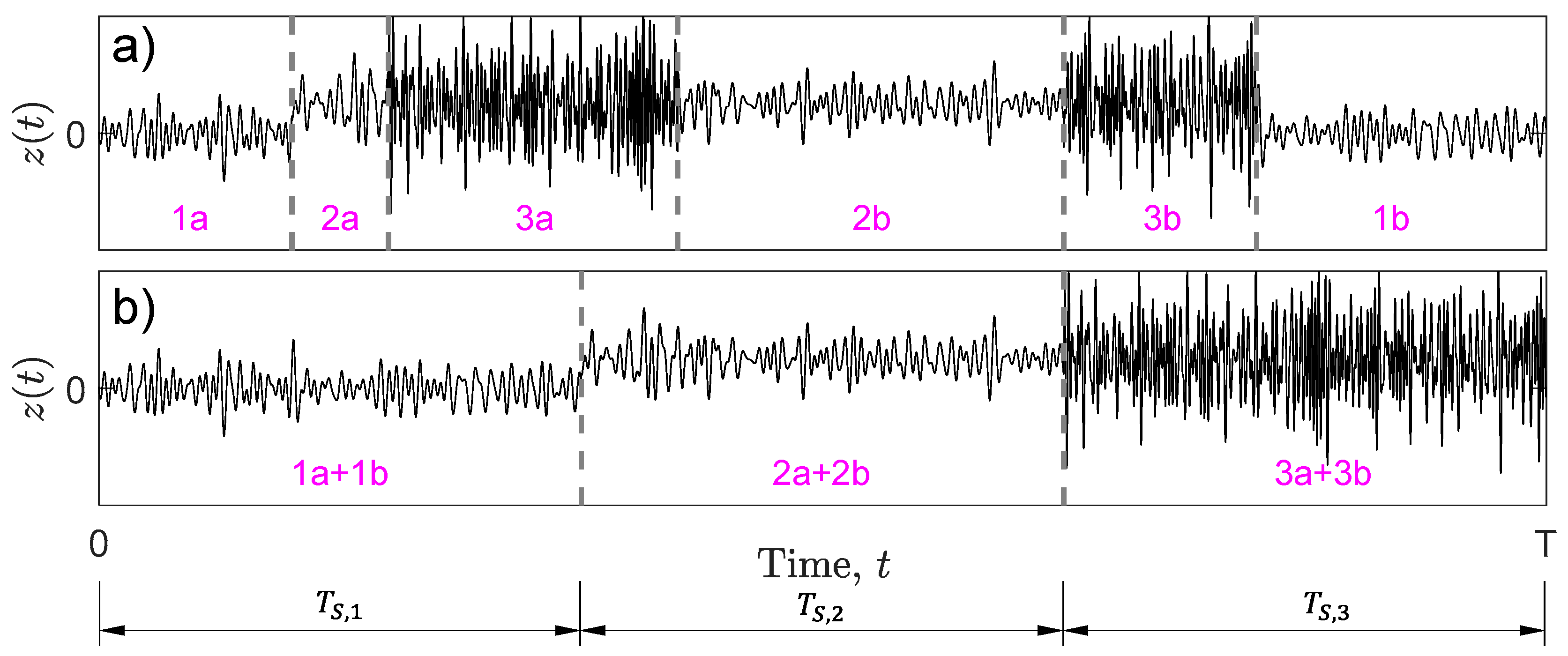
Figure 3.
Load A: three states of same duration ; the values of and are in bottom subplots.
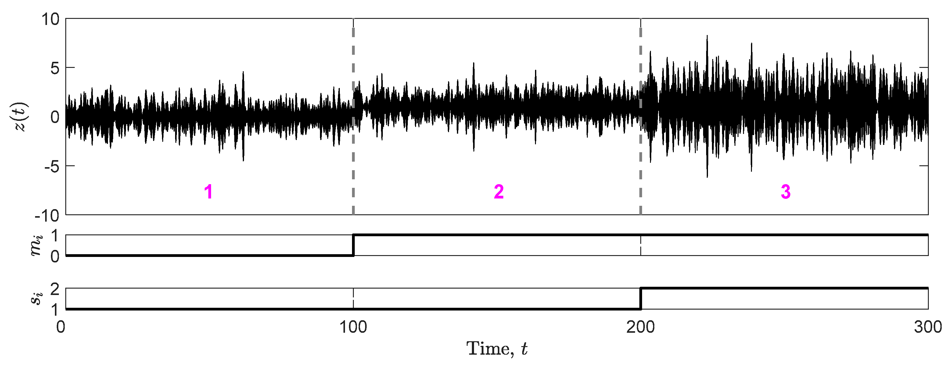
Figure 4.
Load C: (a) with replicated states and (b) after reordering (values of and in bottom subplots).
Figure 4.
Load C: (a) with replicated states and (b) after reordering (values of and in bottom subplots).
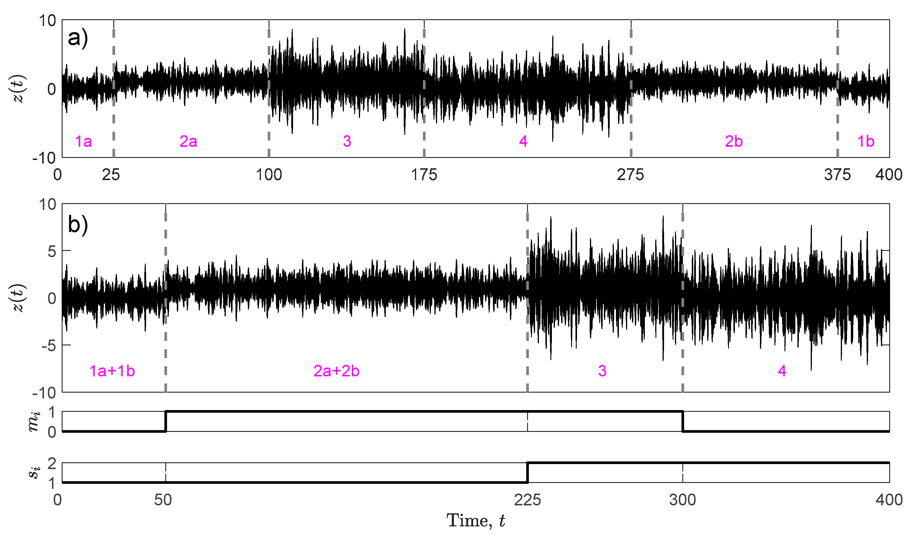
Figure 5.
Load A: (a) confidence intervals versus number of blocks ; (b) sample of 20 confidence intervals for case .
Figure 5.
Load A: (a) confidence intervals versus number of blocks ; (b) sample of 20 confidence intervals for case .
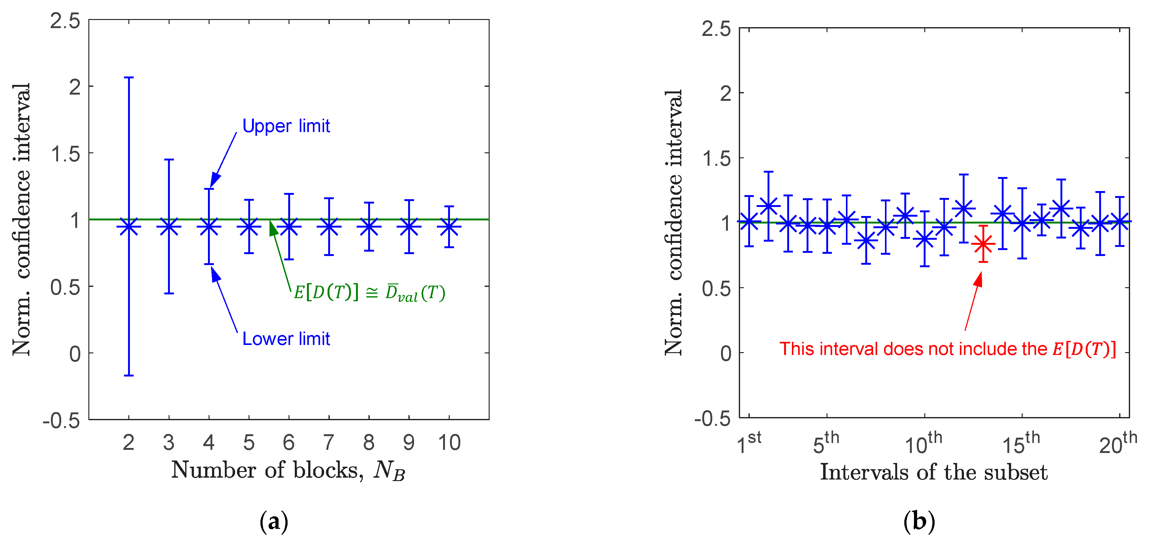
Figure 6.
Instrumented mountain bike used in experiments, with strain gages, data acquisition system, battery and speedometer.
Figure 6.
Instrumented mountain bike used in experiments, with strain gages, data acquisition system, battery and speedometer.
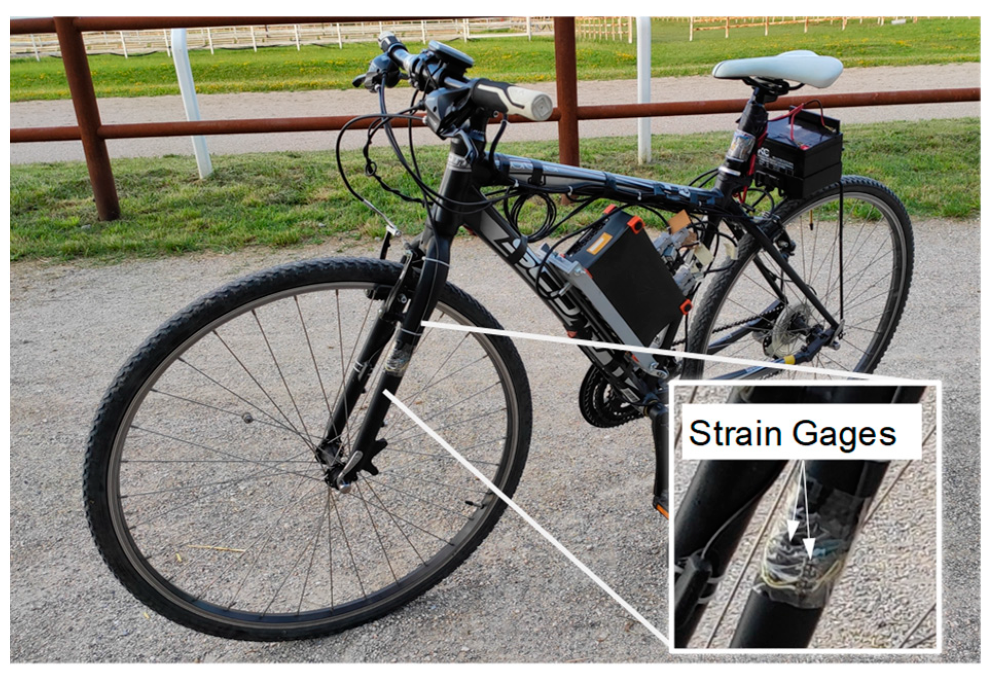
Figure 7.
Overview of track types: (a) gravel surface (stationary case); (b) asphalt, gravel and grass surface (non-stationary case).
Figure 7.
Overview of track types: (a) gravel surface (stationary case); (b) asphalt, gravel and grass surface (non-stationary case).

Figure 8.
Overall and zoom view of measured load records: (a) stationary and (b) non-stationary.
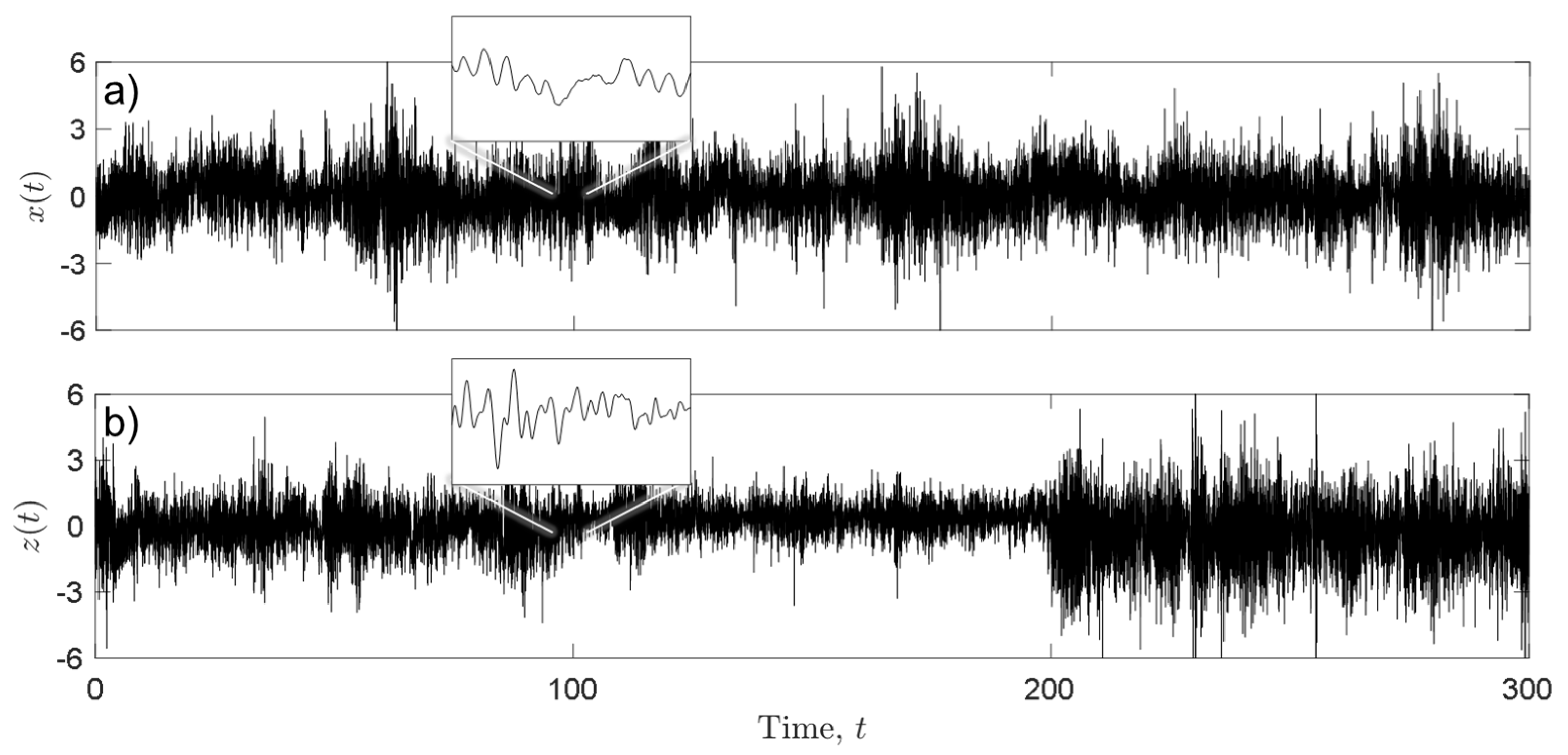
Figure 9.
Run test applied to a measured stress-time history classified as stationary: (a) and (b) .
Figure 9.
Run test applied to a measured stress-time history classified as stationary: (a) and (b) .
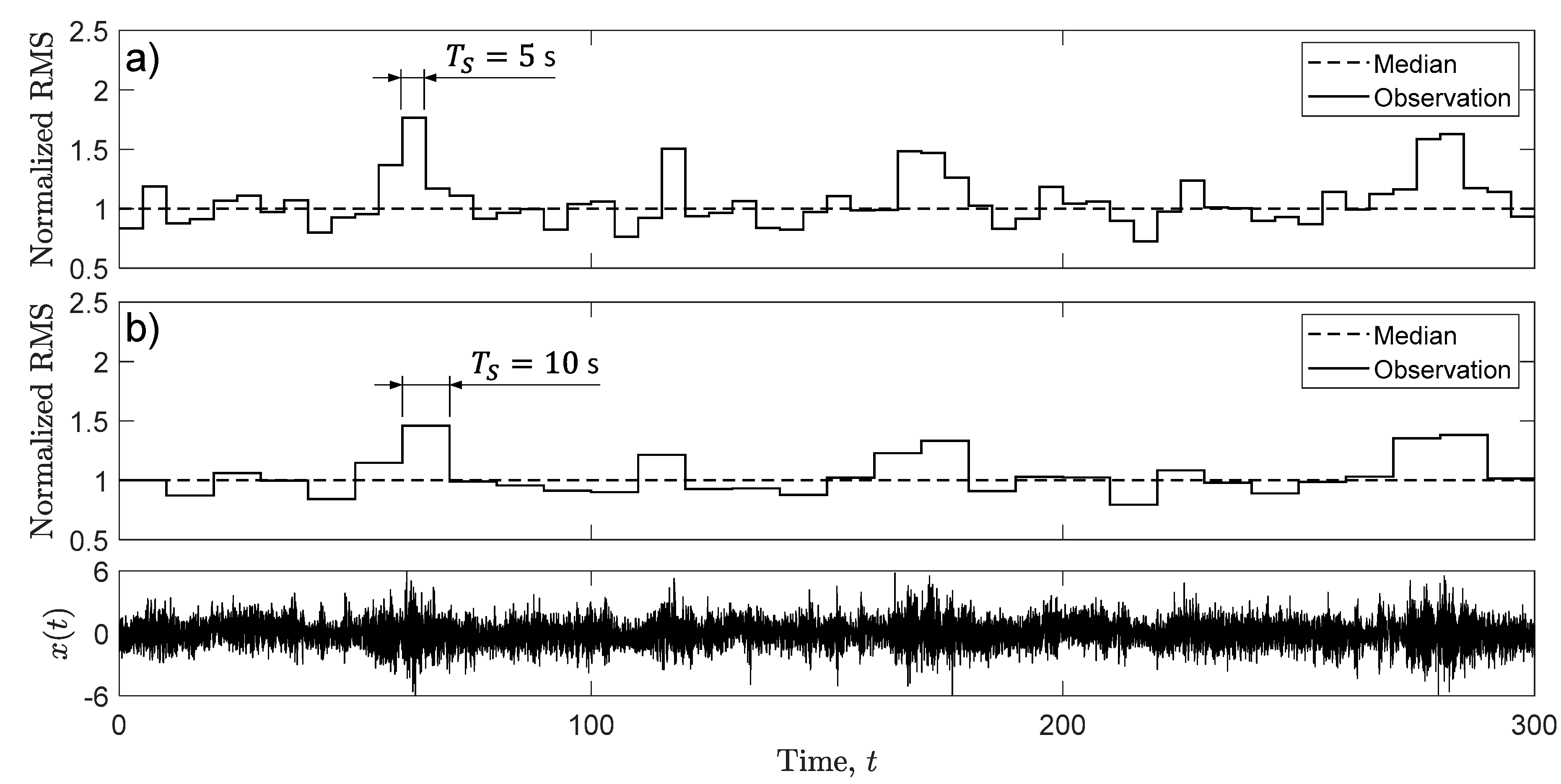
Figure 10.
Run test applied to a measured stress-time history classified as non-stationary: (a) and (b) .
Figure 10.
Run test applied to a measured stress-time history classified as non-stationary: (a) and (b) .
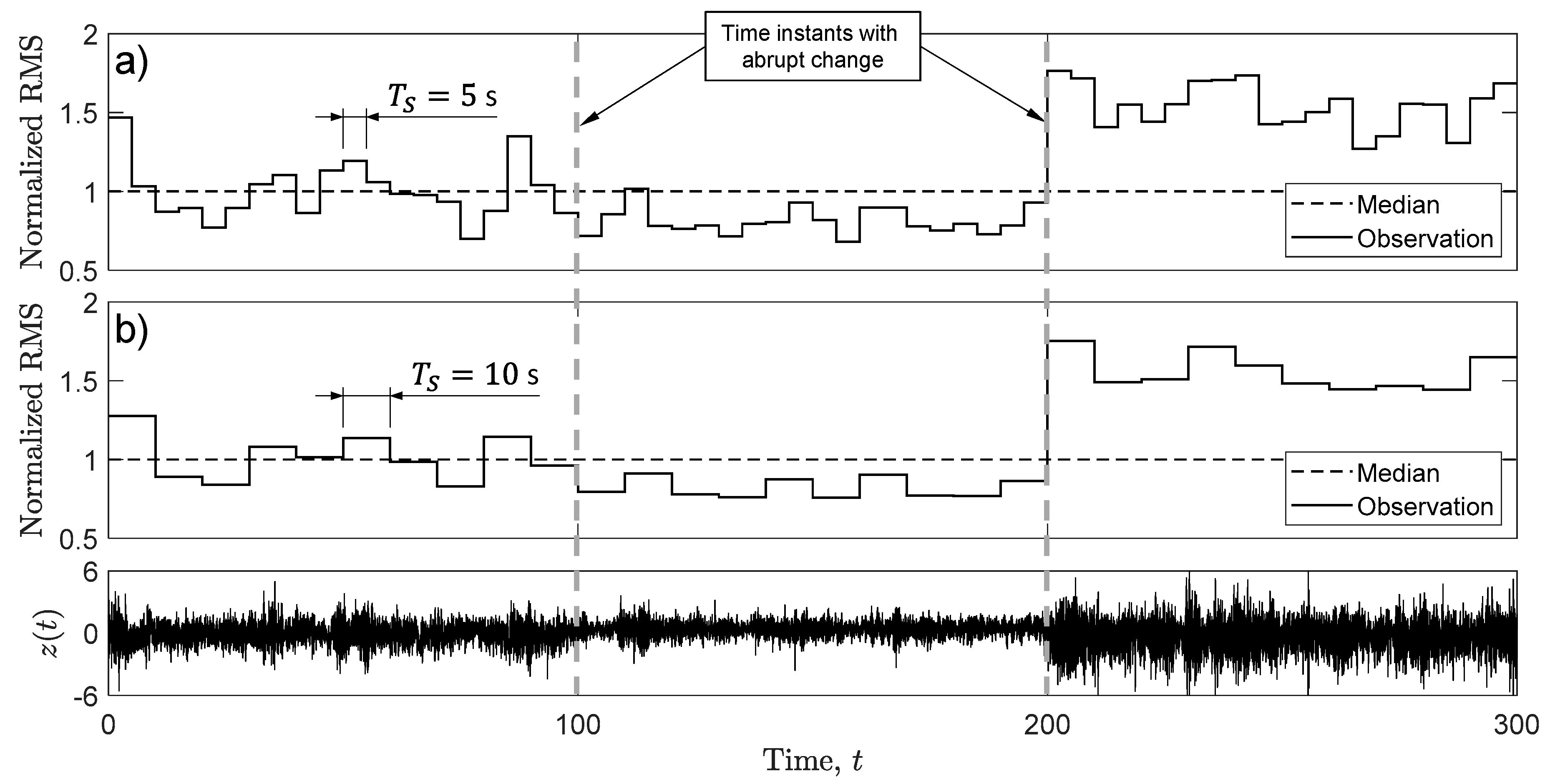
Figure 11.
Confidence intervals for measured stationary stress-time histories as a function of (a) number of records (Case M) and (b) number of subdividing blocks (Case S).
Figure 11.
Confidence intervals for measured stationary stress-time histories as a function of (a) number of records (Case M) and (b) number of subdividing blocks (Case S).
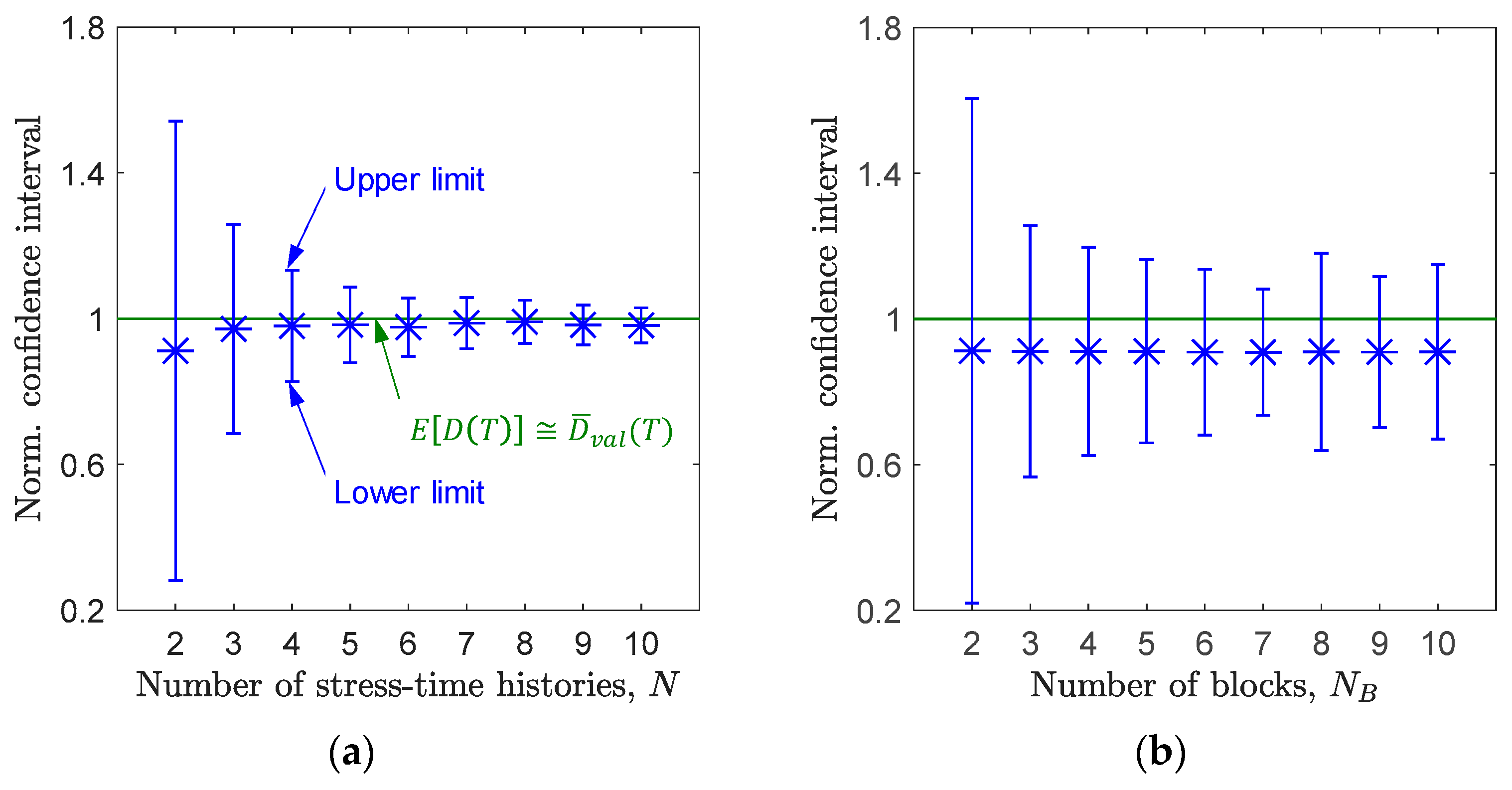
Figure 12.
Confidence interval on expected damage for non-stationary switching loading measured in the mountain bike, as a function of the number of blocks.
Figure 12.
Confidence interval on expected damage for non-stationary switching loading measured in the mountain bike, as a function of the number of blocks.


Table 1.
Combinations of expected value and variance of the first six random variables .
| Parameters | ||||||
|---|---|---|---|---|---|---|
| 1 | 2 | 3 | 4 | 5 | 6 | |
| Expected value, | 0 | 0 | 0 | 0 | 1 | 1 |
| Variance, | 1 | 5 | 10 | 100 | 1 | 5 |
Table 2.
Observed confidence level as a function of the number of random variables and sample size .
Table 2.
Observed confidence level as a function of the number of random variables and sample size .
| 2 | 3 | 4 | 5 | 6 | |
|---|---|---|---|---|---|
| 98.47% | 98.24% | 95.96% | 95.82% | 94.90% | |
| 95.08% | 95.05% | 95.08% | 95.07% | 95.11% | |
| 95.00% | 95.01% | 95.00% | 95.02% | 95.00% | |
Table 3.
Statistics of fatigue damage calculated from measured stationary load records.
| Case M | Case S | ||||
|---|---|---|---|---|---|
| 2 | 0.912 | 1.048 | 2 | 0.913 | 0.814 |
| 3 | 0.972 | 1.727 | 3 | 0.911 | 1.198 |
| 4 | 0.980 | 1.430 | 4 | 0.911 | 1.342 |
| 5 | 0.983 | 1.243 | 5 | 0.911 | 1.353 |
| 6 | 0.977 | 1.138 | 6 | 0.909 | 1.322 |
| 7 | 0.988 | 1.130 | 7 | 0.909 | 1.059 |
| 8 | 0.992 | 1.057 | 8 | 0.910 | 1.712 |
| 9 | 0.983 | 1.062 | 9 | 0.909 | 1.343 |
| 10 | 0.982 | 1.003 | 10 | 0.910 | 1.582 |
Table 4.
Statistics calculated from measured non-stationary stress-time history.
| Statistics for Confidence Intervals | |||
|---|---|---|---|
| 2 | 1.086 | 1 | 0.767 |
| 3 | 1.087 | 2 | 0.559 |
| 4 | 1.083 | 3 | 0.579 |
| 5 | 1.085 | 5 | 0.566 |
| 6 | 1.081 | 7 | 0.506 |
| 7 | 1.081 | 7 | 0.740 |
| 8 | 1.079 | 8 | 0.606 |
| 9 | 1.078 | 10 | 0.651 |
| 10 | 1.076 | 12 | 0.587 |
Disclaimer/Publisher’s Note: The statements, opinions and data contained in all publications are solely those of the individual author(s) and contributor(s) and not of MDPI and/or the editor(s). MDPI and/or the editor(s) disclaim responsibility for any injury to people or property resulting from any ideas, methods, instructions or products referred to in the content. |
© 2023 by the authors. Licensee MDPI, Basel, Switzerland. This article is an open access article distributed under the terms and conditions of the Creative Commons Attribution (CC BY) license (https://creativecommons.org/licenses/by/4.0/).
Share and Cite
MDPI and ACS Style
Marques, J.M.E.; Benasciutti, D.; Papuga, J.; Růžička, M. Uncertainty of Estimated Rainflow Damage in Stationary Random Loadings and in Those Stationary per partes. Appl. Sci. 2023, 13, 2808. https://doi.org/10.3390/app13052808
AMA Style
Marques JME, Benasciutti D, Papuga J, Růžička M. Uncertainty of Estimated Rainflow Damage in Stationary Random Loadings and in Those Stationary per partes. Applied Sciences. 2023; 13(5):2808. https://doi.org/10.3390/app13052808
Chicago/Turabian StyleMarques, Julian M. E., Denis Benasciutti, Jan Papuga, and Milan Růžička. 2023. "Uncertainty of Estimated Rainflow Damage in Stationary Random Loadings and in Those Stationary per partes" Applied Sciences 13, no. 5: 2808. https://doi.org/10.3390/app13052808
Note that from the first issue of 2016, this journal uses article numbers instead of page numbers. See further details here.