
Thermal Characterisation of Automotive-Sized Lithium-Ion Pouch Cells Using Thermal Impedance Spectroscopy

Electrical Energy Storage Technology (EET), Institute of Energy and Automation, Technische Universität Berlin, Einsteinufer 11, D-10587 Berlin, Germany
*
Author to whom correspondence should be addressed.
Appl. Sci. 2023, 13(5), 2870; https://doi.org/10.3390/app13052870
Submission received: 2 February 2023
/
Revised: 16 February 2023
/
Accepted: 21 February 2023
/
Published: 23 February 2023
(This article belongs to the Special Issue Advances in Lithium-Ion Automobile Batteries)
Abstract
:This study used thermal impedance spectroscopy to measure a 46 Ah high-power lithium-ion pouch cell, introducing a testing setup for automotive-sized cells to extract the relevant thermal parameters, reducing the time for thermal characterisation in the complete operational range. The results are validated by measuring the heat capacity using an easy-to-implement calorimetric measurement method. For the investigated cell at 50% state of charge and an ambient temperature of 25 °C, values for the specific heat capacity of 1.25 J/(gK) and the cross-plane thermal conductivity of 0.47 W/(mK) are obtained. For further understanding, the values were measured at different states of charge and at different ambient temperatures, showing a notable dependency only on the thermal conductivity from the temperature of −0.37%/K. Also, a comparison of the cell with a similar-sized 60 Ah high-energy cell is investigated, comparing the influence of the cell structure to the thermal behaviour of commercial cells. This observation shows about 15% higher values in heat capacity and cross-plane thermal conductivity for the high-energy cell. Consequently, the presented setup is a straightforward implementation to accurately obtain the required model parameters, which could be used prospectively for module characterisation and investigating thermal propagation through the cells.
1. Introduction
Ramping up the usage of lithium-ion batteries (LIBs) on a global scale, mainly in the automotive context, requires, besides cell ageing, a broad understanding of both the electrical and the thermal behaviour. Ideal thermal management, especially for large-scale battery systems, is crucial for the maximum possible power and energy supply the system can contribute at a particular state. This optimisation must be done to improve the acceptance of electric vehicles by minimising the required battery cells due to higher power and energy availability without decreasing the driving range.
Thermal characterisation is divided into two general approaches. The first uses external excitation to obtain both the heat capacity (e.g., calorimetric tests [1,2,3]) and the thermal conductivity (e.g., one-sided heat pulses using a calefaction plate [4,5,6] or a flashlight [7,8]). Often these methods require extended auxiliary testing equipment. The other approach uses internal thermal excitation of heat created by the current in the cell. These tests require only standard laboratory equipment and are faster and easier to integrate into battery characterisation procedures.
In this paper, the focus lies on the usage of the latter. Here, the literature introduces and discusses multiple different approaches. The procedures often follow well-known electrical characterisation methods, for instance, pulse response triggered by a direct current as in the hybrid pulse power characterisation [9] or using a sinusoidal current as in electrochemical impedance spectroscopy [10,11].
These testing principles are adjusted to observe the thermal response of the cell [12,13]. Thermal characterisation tests need a longer overall testing time due to the longer time constants, and obtaining an appropriate temperature response often requires high currents, which leads to necessary adaptations in the testing schemes. The state of charge (SOC) plays an essential role in the thermal behaviour of a battery cell. While the parameters of the cell remain nearly constant, as shown in this paper following the literature [14,15,16], the heating of the battery itself differs due to the so-called reversible heat term. Therefore, pulsing the excitation current at a relatively high frequency is often required to maintain a quasi-stationary SOC for obtaining the thermal parameters [17,18,19]. This paper uses thermal impedance spectroscopy (TIS) as an easy-to-implement approach to calculate the battery cell’s heat capacity and thermal conductivity for large-area cells. TIS was first introduced by [12] using an external heating coil to investigate the temperature response of the cell and afterwards adapted by other researchers using internal heating [20,21] to obtain the cell’s parameters. The investigations mostly correspond to smaller cell formats, for example cylindrical [21,22] or small pouch cells [20,23]. This paper firstly investigates and compares two same-sized large-area cells with different cell configurations and capacities, as further described in Section 2.2. Utilising a polystyrene arrangement around the significant cell surfaces in this paper shows that the TIS can be used for automotive-sized cells accordingly while also displaying the cell behaviour in the complete operational range. The results can benefit the implementation of a thermal management system in automotive applications by showing considerable differences in the system behaviour at usage.
2. Materials and Methods
2.1. Test Definitions
A standard test procedure is introduced to cover the relevant thermal cell behaviour. Using the procedure from [20,23], the plan utilises seven measuring points at logarithmically distributed frequencies from 3 mHz as the first measurement point to 160 µHz as the last tested frequency. Also, the number of repetitions per point is changed by modifying the first measuring frequency to 50 repetitions, allowing the cell temperature to reach a quasi-steady state in the first 40 oscillations. A carrier signal utilising a frequency of 5 Hz is overlaid to each corresponding measuring frequency to maintain a stationary state. Here, mainly the testing system defines the carrier frequency.
The frequency band in Table 1 defines the limits of the upcoming spectra. The upper boundary results from the minor measurable temperature response at a particular excitation current and the corresponding generated heat. In contrast, the lower boundary corresponds to the compromise of the overall test duration and the benefit of using lower frequencies to the resulting spectra and fitting. Also, the influence of heating of ambient materials, for instance, the climate chamber and the air around the tested setup, limits the lower end of the test [22]. The first quarter of the resulting data points per frequency for further investigation gets cut out. This results in reducing the number of observed oscillations to seven or three. As described in [20], this adjustment helps to minimise inaccuracies due to a change in the occurring per measurement point.
The paper investigates the cell’s thermal behaviour according to the SOC and ambient temperature. Therefore, a test matrix considering the SOC at 20%, 35%, 50%, 65% and 80% and Tamb of 10 °C, 15 °C, 25 °C, 35 °C and 45 °C is spread out. The SOC starts at 50% in 15% steps in both directions. The limits at 20% and 80% rely on the safety limits of the cell to maintain the cell’s voltage range. The temperature values cover a broad range in which a battery is typically used. Here, the datasheet defines the lower limit at 10 °C. It is the minimum ambient temperature at which a high charging current, as utilised in the test, lies within the safety limits. The upper temperature at 45 °C, again, is a value which lies within the boundaries of the cell datasheet and represents a temperature in a real-world application. A consistent current amplitude is specified at I = 92 A, representing a maximum current of a 2C-rate. The modulated current signal is shown in Figure 1.
The thermal response of the battery cell and the minimum sensor excitation define the current rate since the influence of the noise on the temperature signal at the measurement points on the cell’s surface gets more significant at the higher frequencies caused by less overall generated heat. A direct current offset using a third of the amplitude (Ioff = 30.66 A) is overlaid to minimise extensive cooling of the cell during phases near the zero crossing of the signal [22]. The influence can be seen in Figure 2a, as the minimum heat generation is 0.6 W.
The following Equation (1) usually defines the generated heat . It covers the main heating aspects [24,25]. The first term on the right side describes the irreversible or joule heating using the current and the ohmic resistance . The second term represents the reversible heat by entropic changes during the change of the SOC. Here, the temperature and the open circuit voltage are further introduced:
As mentioned above, reversible heat is excluded as a quasi-stationary SOC is maintained. That leads to heat generation independent of the current direction, shown in Equation (2):
The resulting heat generation is shown for the 160 µHz frequency in Figure 2a and the corresponding temperature response in Figure 2b. The timeframe on both x-axes represents the actual test time while measuring this frequency point. The data are then preprocessed utilising the envelope function and a second-order sinus fit created by the quadratic current to acquire the maximum value for both the heat generation and the temperature response and the phase shift between both. The values lead to the thermal impedance calculated by Equation (3), using as the phase shift between the generated heat and the temperature response at a particular frequency:
2.2. Cell Setup
This paper investigates a 46 Ah LIB pouch cell of the manufacturer Kokam. The cell consists of a nickel–manganese–cobalt cathode and is built in a high-power (HP) configuration using wider current collectors and thinner layers of active material. This composition must be considered when comparing results to other test results. The cell measures 226 × 225 × 12 mm. Excluding the weld results in a width of w = 210 mm and a height of h = 190 mm. Figure 3 schematically shows the arrangement of seven used PT100 temperature sensors on the cell surface. The locations are shown in relative values due to better reproducibility using cells in different shapes. In the middle of the cell, a sensor is attached to both sides of the battery cell. This arrangement covers the validation for equal heat distribution in both directions perpendicular to the layers. The same test procedure was replicated as a reference using an equal-sized 60 Ah cell in a high-energy (HE) arrangement.
Figure 4 shows the overall setup. Here, two plates of polystyrene with a thickness of 30 mm each cover the two wider sides of the cell. To hold these plates in place and to apply an equal pressure all over the cell’s surface, two identical polyvinyl chloride plates of a thickness of 10 mm are attached and moderately compressed by six equally distributed springs. The tests were conducted using a BasyTec MRS cell cycler and a Memmert ICP110 climate chamber to obtain a constant ambient condition at particular temperatures.
2.3. Model Approach
The simplest model to describe the thermal behaviour of the battery cell is a first-order Cauer model. This kind of model corresponds with an RC element in system theory. Often the scope of that model is enough to feedback on the system response to a specific current signal of an electric model. Here, the model is adjusted for the system in Figure 5. The approach requires assumptions. For instance, heat generation and the heat capacity’s Cp location occur in the cell’s volumetric centre. Also, the heat transfer in both cross-plane directions, meaning towards the large-area surfaces, is equally distributed. This simplifies the overall model setup, like dividing the internal thermal resistance into two similar parts. Polystyrene plates cover the outer boundaries of the battery, as shown in Figure 4. In the model, these also simplify as single resistances, , excluding the heat capacity of the plates assuming the impact is negligible. The value can be calculated since all material constants and dimensions are known. Considering Figure 4, the temperature measurement points lie between the cell surface and the individual polystyrene plates. In Figure 5, these points are marked as Tsur,up and Tsur,down, respectively. The conditions inside the climate chamber are assumed to be homogeneous in the whole chamber. Therefore, the ambient temperature Tamb on all sides of the setup is set to be equal.
The measured spectra need to be fitted to extract the cell’s heat capacity and thermal conductivity in a cross-plane direction. This approach implements a least-squares fitting algorithm utilising an RC element as the model equation. Therefore, two unknown values, the time constant τ and the resistance value , are fitted. When neglecting the impact of additional heat capacities, like the polystyrene plates and the effect of the temperature sensors, as discussed later, the cell’s heat capacity is calculated by = τ/. Dividing the resulting value by the cell mass gives the specific heat capacity cp = /mcell.
The fitted value , representing the overall thermal resistance, is adapted to obtain the cross-plane thermal conductivity . As described above, the system assumes an equal heat distribution at the top and the bottom. This postulation is required to simplify the model’s calculation to only one dimension by two resistive elements ( and ). At the measurement point Tsur, both and are connected in parallel:
Therefore, as shown in Equation (4), it is necessary to calculate from the fitted by subtracting the known thermal resistance of the polystyrene plate. Afterwards, the resulting is divided by two, assuming an equal heat dissipation in both cross-plane directions of the cell. Finally, converting the final thermal resistance by the dimensions results in the cell’s cross-plane heat conductivity using as the cell thickness and as the cell area in the following Equation (5):
2.4. Calorimetric Reference Test
The characterisation method described by [26] using a pseudo-calorimetric reference test was conducted to get reference values for the specific heat capacity of the tested cells. The testing scheme requires a reference material with known thermal properties. In this case, an aluminium plate with dimensions similar to the battery cell surface was used. The test utilises an insulation setup, as shown in Figure 6a, using a polystyrene casing with a cut-off in the object’s size to minimise convection and radiation. In the first step, the setup is heated in the climate chamber to a steady-state temperature of Tamb = 50 °C with the aluminium plate inserted. After temperature sensors on the object surface inside the polystyrene casing show the same steady-state temperature, the chamber switches off. The resulting temperature decrease is recorded inside the insulation (Ts) and in ambient conditions inside the climate chamber (Tamb). Afterwards, the battery cell is inserted, conducting the same test procedure. This test does not need prior information on the heat flow. The calculation of the resulting heat capacity is described in [26], fitting the logarithmic temperature difference = Ts − Tamb as shown in Figure 6b.
3. Results
In the first step, multiple pre-tests characterising the cell’s behaviour under different ambient conditions are conducted before sampling the test matrix. The main adaptions are presented and compared using the concluding spectra. Due to better visualisation, all upcoming spectra are shown with linear interpolated graphs in a Nyquist plot. If not mentioned further, the given spectrum shows the results for the upper measurement point in the cell’s centre.
3.1. Pre-Tests
The setup’s symmetry must be confirmed to utilise the model generalisation described in Section 2. The spectra shown in Figure 7 represent the measurement points above (red) and underneath (green) the cell. The behaviour of both positions exhibits a similar result. The differences in the specific heat capacity and the cross-plane thermal conductivity stay in a range of less than 2% for all performed tests. For further evaluation, both corresponding values from above and below the cell are averaged.
The frequency band is mainly defined by comparing two tests using different lower boundaries. Adding two additional frequencies at 100 µHz and 50 µHz, as described in Table 1, results in the red-coloured spectrum in Figure 8. Comparing the extended spectrum to a standard test using the Nyquist plot in Figure 8a and the Bode plot in Figure 8b also shows good test repeatability.
Both tests show practically similar values; especially the specific heat capacity is roughly the same. When averaging both central measurement points above and underneath the cell, the difference between both tests stays lower than 1%. The difference between the cross-plane thermal conductivities shows a higher deviation of approximately 7%. The thermal influence of the surroundings causes these variations as the heating phases become longer. Therefore, a higher overall temperature increase results in a smaller general thermal resistance and a higher corresponding thermal conductivity while testing lower frequencies.
3.2. Comparision to Reference Test and Other Cell Configurations
The calorimetric test procedure defined in the materials section validates the results given by the TIS schedule. Also, a comparison to an HE cell using the same geometrical format as the observed cell is investigated.
In Figure 9, the resulting impedance spectra of both cells are shown. Here, the higher the temperature response per generated heat is, the larger the resulting semi-circle becomes. That mainly results from a smaller heat capacity of the cell, causing a more elevated temperature increase. As expected, the HE cell also shows a smaller cross-plane heat conductivity resulting from the different layer thicknesses. Especially the thinner current collectors of HE cells made of proper thermal conductive materials (aluminium and copper) and thicker active materials decrease the overall cross-plane heat conductivity.
Comparing the results of both cells in Table 2 shows the expected behaviour, using a standard ambient configuration of Tamb = 25 °C and a SOC of 50% each. The specific heat capacity shows a difference of nearly 13%, while the cross-plane heat conductivity differs by approximately 16%. For both values, the HP cell delivers the surplus. When comparing both cell types using the calorimetric test setup, the difference between the cells is reduced, showing a difference of only 3%. A possible reason is the setup used, which is highly dependent on the polystyrene casing. Moreover, the influence of the surrounding air in the climate chamber is more prominent here. Also, a deviation of less than 2% for the further investigated HP cell between the TIS and the calorimetric test can be observed. Considering the HE cell, the difference is almost 9%.
3.3. Analysis of Cell Behaviour
After finishing the pre-tests and the reference schedules using a similar-sized cell and a calorimetric test alternative, the decisive test matrix covering the SOC and temperature dependency was carried out. This involved repeating the standard test procedure at the different cell states, investing five SOCs, starting at a minimum value of 20% and increasing in 15% steps. Also, the test matrix stretched further, covering five temperature measurement points from 10 °C to 45 °C per SOC.
In Figure 10, the parameter adaptation is compared. On the left-hand side, in Figure 10a, the SOC differs at a standard temperature of 25 °C, while in the right plot (Figure 10b), the temperature varies at fixed SOC of 50%. Here, the temperature impact appears to be more influential to the battery cell. In contrast, the SOC shows nearly no particular significance, while the impedance spectrum becomes larger when increasing the ambient temperature. That impact results from the smaller total heat generated due to a decreasing ohmic resistance of the cell when increasing the temperature.
The results show that neither the specific heat capacity nor thermal conductivity indicate a significant dependency on the SOC [12,18,27,28]. The model approach in Figure 5 is simplified to extract the parameter from the calculated spectra. In this paper, the relevant values for the heat capacity and thermal resistance are fitted using a first-order Cauer model, representing a single RC element, as shown in the upper graphic in Figure 11b. The thermal resistance is then converted to the cross-plane thermal conductivity, further described in Section 2.3. Figure 11a compares a first- and second-order fit to the data points. The fit shows good overall accordance with the data. Furthermore, it shows only insignificant changes in the resulting values comparing a first-order model (Figure 11b, top) to a second-order model (Figure 11b, bottom). Here, the second-order model simulates the time delay caused by the temperature sensor and other surroundings. Given the minor influence of that additional time constant, the fitting algorithm is not adapted to that behaviour.
Figure 12 presents both values as a function of SOC for all temperature measurement points. The thermal conductivity in Figure 12b shows nearly constant values, while the specific heat capacity in Figure 12a shows slightly different behaviour for the higher two temperatures. The specific heat capacity scarcely increases with SOC at higher temperatures. This can be caused by the rising negative real part of the Nyquist diagram (Figure 10b), which is not a part of the general RC fit in this work. Here, the influence of the sensor and different surroundings are more significant.
Overall, the average specific heat capacity values differ from 1.22 J g−1 K−1 (SOC = 50% and T = 25 °C) to 1.35 J g−1 K−1 (SOC = 80% and T = 35 °C), showing a maximum spread of approximately 10%. The average value inside the test matrix is 1.27 J g−1 K−1. Regarding the cross-plane thermal conductivity, the values vary by nearly 28% from 0.38 W m−1 K−1 (SOC = 65% and T = 45 °C) to 0.53 W m−1 K−1 (SOC = 35% and T = 10 °C), with an average value of 0.47 W m−1 K−1.
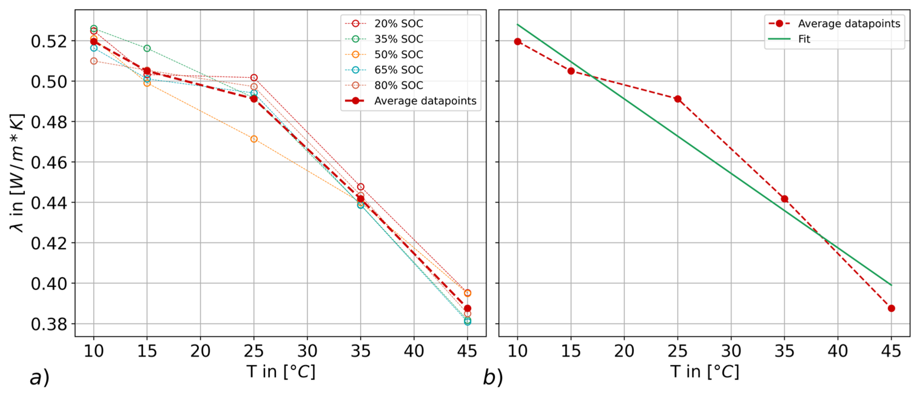
While the specific heat capacity remains nearly unchanged at the different used states, the cross-plane thermal conductivity negatively correlates with temperature, as shown in Figure 13a. That correlation was also observed in [5,8,18,29]. In Figure 13b, the average over each SOC per temperature point was used to obtain the function gain by a linear fit. Here, the correlation is −0.37%/K for λ⊥.
4. Discussion
The resulting values for the specific heat capacity and the cross-plane thermal conductivity indicate a higher correlation of the thermal model parameters to the ambient temperature than to the SOC. Also, the specific heat capacity shows a more consistent behaviour [26,30,31,32]. The averaged cp concerning the SOC differs by 2.2% for all tests, showing slightly higher results for higher SOCs. The different averaged values by the temperature show a deviation of 6.5%, peaking at 35 °C as shown in Figure 12a. Furthermore, the information in Figure 12b shows the rising influence of higher Tamb on the test results. This leads back to the TIS testing schedule and the resulting temperature response due to less heat generated by a decreased ohmic resistance at higher temperatures.
Examining the cross-plane thermal conductivity showed a more significant reliance on external conditions. While averaging the results per SOC, a minor deviation of 2.3% emerges, compared to the crucial impact of Tamb. Here, the difference of 21.1% between the averaged values at 10 °C and 45 °C shows a linear dependency [33,34] decreasing by −0.37%/K. Steinhardt et al. [18] also detected a similar behaviour using different measurement methods. A possible reason is the thermal contact resistance, as discussed in [5,18]. In contrast, [3] did not observe such changes using lithium–iron–phosphate cells, leading to the assumption that the changes are highly dependent on cell chemistry. Thus, further investigations, not in the scope of this work, need to be conducted, especially considering these matters.
Some considerations towards the applicability of the TIS have to be made, especially regarding the negative real part in the Nyquist plot. This behaviour represents at least a second heat capacity in the setup, further illustrated in the phase response of Figure 7b, showing a phase angle of less than −90°. An additional phase shift is caused by the impact of temperature measurements using physically contacted sensors [22], like the PT100 in this work. Also, the surroundings have to be considered in this context since every material has a heat capacity, which influences the resulting spectra.
In this paper, the used model relies on a single RC element using only the heat capacity of the battery, which gives the primary response to the heat generated. In the electrical domain, models are usually described by the Foster model, utilising components connected in series. Here, every element can be more precisely distinguished. The thermal behaviour needs to be modelled differently to maintain the physical representation by the Cauer model, as shown in Figure 11b. The difference lies in the arrangement of the components, which are nested here. This concludes with the given thermal response and the caused spectra showing the aforementioned negative real part, representing a phase shift of more than −90°.
To summarise, the negative part cannot be represented using the fitting function. However, this is neglected here since the influence (supposedly from the sensor) only changes the result insignificantly, as recorded in the literature [20,21,23]. Since a quasi-stationary state is reached at the beginning of the test schedule by increasing the length of the first measurement point, the cell’s behaviour does not depend on the test schedule beforehand. That is important for further usage of TIS as an addition to standard battery check-up tests, using only slight adaptions to the test setup and increasing the testing time by approximately one day. The test is easily reproducible, showing only minor derivation over the conducted tests, for instance, while comparing the frequency bands in Figure 8. The test results mainly differ when changing the test setup or using another overall test setup, which causes changes in the thermal resistance, , which covers the heat transfer to the surroundings.
Investigating the different measured data points, shown in Figure 3, leads to the expected cell conditions. This concludes in decreasing specific heat capacity and increasing cross-plane thermal conductivity the closer the measurement point comes to the tabs and vice versa. The leading cause is the current distribution inside the cell, which is higher at the tabs and lower at the distal ends of the battery cell [35,36,37,38], causing faster and more significant heating at higher current rate locations. That aspect also needs to be considered regarding upcoming thermal management systems.
5. Conclusions
Overall, the technique presented in this paper shows the possibility of using the TIS to characterise even large-format LIBs besides decreasing the overall testing time for more direct implementation in battery characterisation methods. A follow-up to the described approach can include investigating battery modules to identify the heat propagation from one cell to the next and the temperature gradients going along with it. Moreover, the influence of the cell sizing and the impact of the cell configuration as HE or HP need to be regarded in more detail in upcoming work.
Author Contributions
Conceptualization, D.D.; methodology, D.D.; software, D.D.; validation, D.D.; formal analysis, D.D.; investigation, D.D.; resources, D.D.; data curation, D.D.; writing—original draft preparation, D.D. and J.K.; writing—review and editing, D.D. and J.K.; visualization, D.D.; supervision, J.K.; project administration, D.D. and J.K.; funding acquisition, J.K. All authors have read and agreed to the published version of the manuscript.
Funding
This research was funded by Federal Ministry for Economic Affairs and Energy (BMWE), grant number 03ETE033B.
Institutional Review Board Statement
Not applicable.
Informed Consent Statement
Not applicable.
Data Availability Statement
Not applicable.
Conflicts of Interest
The authors declare no conflict of interest.
References
- Nieto, N.; Díaz, L.; Gastelurrutia, J.; Alava, I.; Blanco, F.; Carlos Ramos, J.; Rivas, A. Thermal Modeling of Large Format Lithium-Ion Cells. J. Electrochem. Soc. 2013, 160, A212–A217. [Google Scholar] [CrossRef]
- Vertiz, G.; Oyarbide, M.; Macicior, H.; Miguel, O.; Cantero, I.; Fernandez de Arroiabe, P.; Ulacia, I. Thermal characterization of large size lithium-ion pouch cell based on 1d electro-thermal model. J. Power Sources 2014, 272, 476–484. [Google Scholar] [CrossRef]
- Bazinski, S.J.; Wang, X. Experimental study on the influence of temperature and state-of-charge on the thermophysical properties of an LFP pouch cell. J. Power Sources 2015, 293, 283–291. [Google Scholar] [CrossRef]
- Aiello, L.; Kovachev, G.; Brunnsteiner, B.; Schwab, M.; Gstrein, G.; Sinz, W.; Ellersdorfer, C. In Situ Measurement of Orthotropic Thermal Conductivity on Commercial Pouch Lithium-Ion Batteries with Thermoelectric Device. Batteries 2020, 6, 10. [Google Scholar] [CrossRef]
- Steinhardt, M.; Gillich, E.I.; Stiegler, M.; Jossen, A. Thermal conductivity inside prismatic lithium-ion cells with dependencies on temperature and external compression pressure. J. Energy Storage 2020, 32, 101680. [Google Scholar] [CrossRef]
- Cheng, X.; Tang, Y.; Wang, Z. Thermal Property Measurements of a Large Prismatic Lithium-ion Battery for Electric Vehicles. J. Therm. Sci. 2021, 30, 477–492. [Google Scholar] [CrossRef]
- Parker, W.J.; Jenkins, R.J.; Butler, C.P.; Abbott, G.L. Flash Method of Determining Thermal Diffusivity, Heat Capacity, and Thermal Conductivity. J. Appl. Phys. 1961, 32, 1679–1684. [Google Scholar] [CrossRef]
- Arzberger, A.; Hellenbrand, M.; Sauer, D.U. The change of thermal conductivity of Lithium-Ion pouch cells with operating point and what this means for battery thermal management. In Proceedings of the AABC 2014—Advanced Automotive Battery Confernce, Atlanta, GA, USA, 15–19 June 2014. [Google Scholar]
- Thanagasundram, S.; Arunachala, R.; Makinejad, K.; Teutsch, T.; Jossen, A. A Cell Level Model for Battery Simulation. In Proceedings of the European Electric Vehicle Congress 2012, Brussels, Belgium, 20–22 November 2012. [Google Scholar]
- Popkirov, G.S.; Schindler, R.N. A new impedance spectrometer for the investigation of electrochemical systems. Rev. Sci. Instrum. 1992, 63, 5366–5372. [Google Scholar] [CrossRef]
- Suresh, P.; Shukla, A.K.; Munichandraiah, N. Temperature dependence studies of a.c. impedance of lithium-ion cells. J. Appl. Electrochem. 2002, 32, 267–273. [Google Scholar] [CrossRef]
- Barsoukov, E.; Jang, J.H.; Lee, H. Thermal impedance spectroscopy for Li-ion batteries using heat-pulse response analysis. J. Power Sources 2002, 109, 313–320. [Google Scholar] [CrossRef]
- Bryden, T.S.; Dimitrov, B.; Hilton, G.; Ponce de León, C.; Bugryniec, P.; Brown, S.; Cumming, D.; Cruden, A. Methodology to determine the heat capacity of lithium-ion cells. J. Power Sources 2018, 395, 369–378. [Google Scholar] [CrossRef]
- Bernardi, D.; Pawlikowski, E.; Newman, J. A General Energy Balance for Battery Systems. J. Electrochem. Soc. 1985, 132, 5–12. [Google Scholar] [CrossRef]
- Viswanathan, V.V.; Choi, D.; Wang, D.; Xu, W.; Towne, S.; Williford, R.E.; Zhang, J.-G.; Liu, J.; Yang, Z. Effect of entropy change of lithium intercalation in cathodes and anodes on Li-ion battery thermal management. J. Power Sources 2010, 195, 3720–3729. [Google Scholar] [CrossRef]
- Eddahech, A.; Briat, O.; Vinassa, J.-M. Thermal characterization of a high-power lithium-ion battery: Potentiometric and calorimetric measurement of entropy changes. Energy 2013, 61, 432–439. [Google Scholar] [CrossRef]
- Tang, Y.; Li, T.; Cheng, X. Review of Specific Heat Capacity Determination of Lithium-Ion Battery. Energy Procedia 2019, 158, 4967–4973. [Google Scholar] [CrossRef]
- Steinhardt, M.; Gillich, E.I.; Rheinfeld, A.; Kraft, L.; Spielbauer, M.; Bohlen, O.; Jossen, A. Low-effort determination of heat capacity and thermal conductivity for cylindrical 18650 and 21700 lithium-ion cells. J. Energy Storage 2021, 42, 103065. [Google Scholar] [CrossRef]
- Kovachev, G.; Astner, A.; Gstrein, G.; Aiello, L.; Hemmer, J.; Sinz, W.; Ellersdorfer, C. Thermal Conductivity in Aged Li-Ion Cells under Various Compression Conditions and State-of-Charge. Batteries 2021, 7, 42. [Google Scholar] [CrossRef]
- Schmidt, J.P.; Manka, D.; Klotz, D.; Ivers-Tiffée, E. Investigation of the thermal properties of a Li-ion pouch-cell by electrothermal impedance spectroscopy. J. Power Sources 2011, 196, 8140–8146. [Google Scholar] [CrossRef]
- Fleckenstein, M.; Fischer, S.; Bohlen, O.; Bäker, B. Thermal Impedance Spectroscopy—A method for the thermal characterization of high power battery cells. J. Power Sources 2013, 223, 259–267. [Google Scholar] [CrossRef]
- Keil, P.; Rumpf, K.; Jossen, A. Thermal Impedance Spectroscopy for Li-Ion Batteries with an IR Temperature Sensor System. World Electr. Veh. J. 2013, 6, 581–591. [Google Scholar] [CrossRef]
- Swierczynski, M.; Stroe, D.I.; Stanciu, T.; Kær, S.K. Electrothermal impedance spectroscopy as a cost efficient method for determining thermal parameters of lithium ion batteries: Prospects, measurement methods and the state of knowledge. J. Clean. Prod. 2017, 155, 63–71. [Google Scholar] [CrossRef]
- Thomas, K.E.; Newman, J. Heats of mixing and of entropy in porous insertion electrodes. J. Power Sources 2003, 119–121, 844–849. [Google Scholar] [CrossRef]
- Catherino, H.A. Estimation of the heat generation rates in electrochemical cells. J. Power Sources 2013, 239, 505–512. [Google Scholar] [CrossRef]
- Maleki, H.; Hallaj, S.A.; Selman, J.R.; Dinwiddie, R.B.; Wang, H. Thermal Properties of Lithium-Ion Battery and Components. J. Electrochem. Soc. 1999, 146, 947–954. [Google Scholar] [CrossRef]
- Bazinski, S.J.; Wang, X. Predicting heat generation in a lithium-ion pouch cell through thermography and the lumped capacitance model. J. Power Sources 2016, 305, 97–105. [Google Scholar] [CrossRef]
- Steinhardt, M.; Barreras, J.V.; Ruan, H.; Wu, B.; Offer, G.J.; Jossen, A. Meta-analysis of experimental results for heat capacity and thermal conductivity in lithium-ion batteries: A critical review. J. Power Sources 2022, 522, 230829. [Google Scholar] [CrossRef]
- Bazinski, S.J.; Wang, X.; Sangeorzan, B.P.; Guessous, L. Measuring and assessing the effective in-plane thermal conductivity of lithium iron phosphate pouch cells. Energy 2016, 114, 1085–1092. [Google Scholar] [CrossRef]
- Sheng, L.; Su, L.; Zhang, H. Experimental determination on thermal parameters of prismatic lithium ion battery cells. Int. J. Heat Mass Transf. 2019, 139, 231–239. [Google Scholar] [CrossRef]
- Schuster, E.; Ziebert, C.; Melcher, A.; Rohde, M.; Seifert, H.J. Thermal behavior and electrochemical heat generation in a commercial 40 Ah lithium ion pouch cell. J. Power Sources 2015, 286, 580–589. [Google Scholar] [CrossRef]
- Andre, D.; Meiler, M.; Steiner, K.; Wimmer, C.; Soczka-Guth, T.; Sauer, D.U. Characterization of high-power lithium-ion batteries by electrochemical impedance spectroscopy. I. Experimental investigation. J. Power Sources 2011, 196, 5334–5341. [Google Scholar] [CrossRef]
- Moitsheki, R.J.; Rowjee, A. Steady Heat Transfer through a Two-Dimensional Rectangular Straight Fin. Math. Probl. Eng. 2011, 2011, 826819. [Google Scholar] [CrossRef]
- Khani, F.; Ahmadzadeh Raji, M.; Hamedi-Nezhad, S. A series solution of the fin problem with a temperature-dependent thermal conductivity. Commun. Nonlinear Sci. Numer. Simul. 2009, 14, 3007–3017. [Google Scholar] [CrossRef]
- Lin, J.; Chu, H.N.; Howey, D.A.; Monroe, C.W. Multiscale coupling of surface temperature with solid diffusion in large lithium-ion pouch cells. Commun. Eng. 2022, 1, 1. [Google Scholar] [CrossRef]
- Nascimento, M.; Paixão, T.; Ferreira, M.; Pinto, J. Thermal Mapping of a Lithium Polymer Batteries Pack with FBGs Network. Batteries 2018, 4, 67. [Google Scholar] [CrossRef]
- Goutam, S.; Timmermans, J.-M.; Omar, N.; Bossche, P.; van Mierlo, J. Comparative Study of Surface Temperature Behavior of Commercial Li-Ion Pouch Cells of Different Chemistries and Capacities by Infrared Thermography. Energies 2015, 8, 8175–8192. [Google Scholar] [CrossRef]
- Zhu, Y.; Xie, J.; Pei, A.; Liu, B.; Wu, Y.; Lin, D.; Li, J.; Wang, H.; Chen, H.; Xu, J.; et al. Fast lithium growth and short circuit induced by localized-temperature hotspots in lithium batteries. Nat. Commun. 2019, 10, 2067. [Google Scholar] [CrossRef]
Figure 1.
Section of modulated current signal for 160 µHz data point. (a) General behaviour, showing the amplitude and the offset; (b) zoomed data to show the 5 Hz carrier signal overlaid to the tested frequency.
Figure 1.
Section of modulated current signal for 160 µHz data point. (a) General behaviour, showing the amplitude and the offset; (b) zoomed data to show the 5 Hz carrier signal overlaid to the tested frequency.
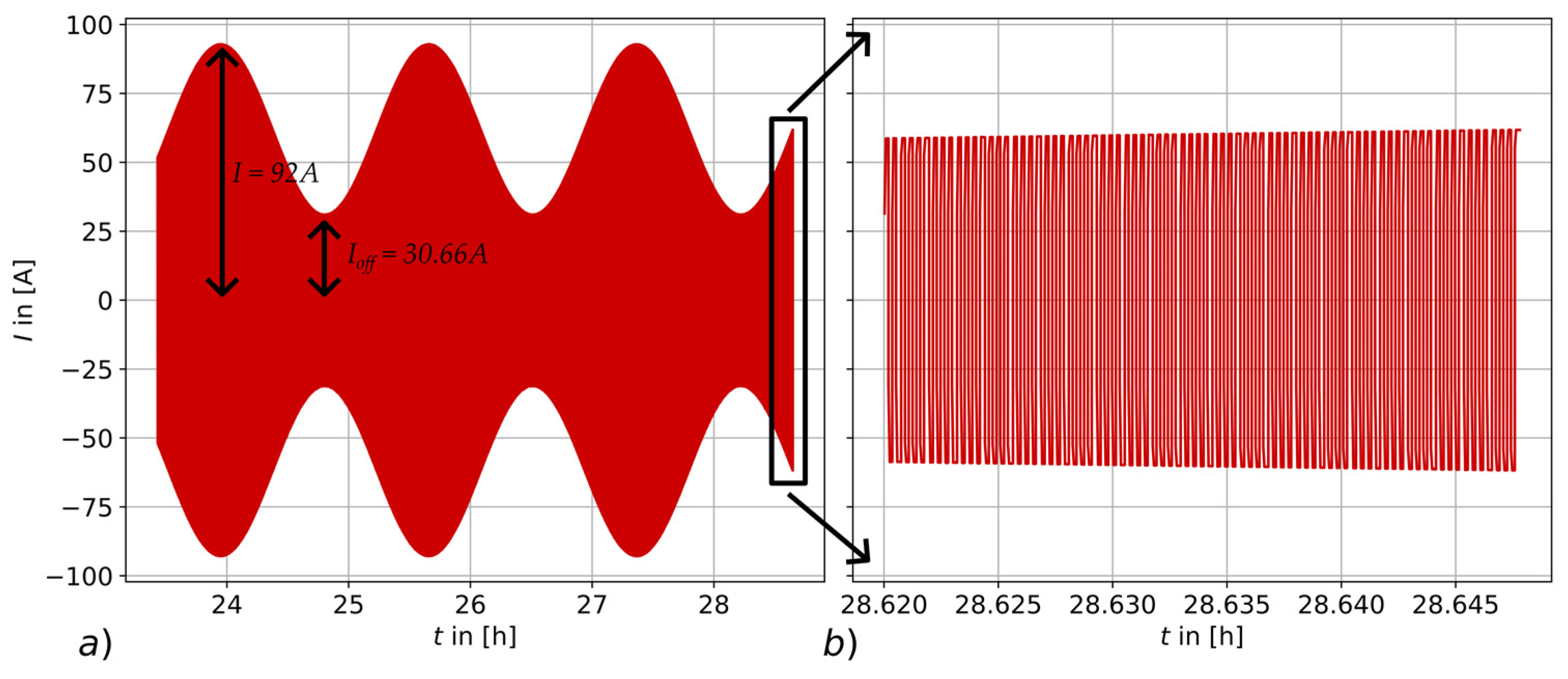
Figure 2.
Section of real measured data for 160 µHz data point. (a) Dissipated heat by irreversible heat; (b) measured thermal response on the centre of the cell’s surface caused by the corresponding heating in (a).
Figure 2.
Section of real measured data for 160 µHz data point. (a) Dissipated heat by irreversible heat; (b) measured thermal response on the centre of the cell’s surface caused by the corresponding heating in (a).

Figure 3.
Locations of temperature measurement points.

Figure 4.
Depiction of test setup.

Figure 5.
Representation of utilised model configuration.
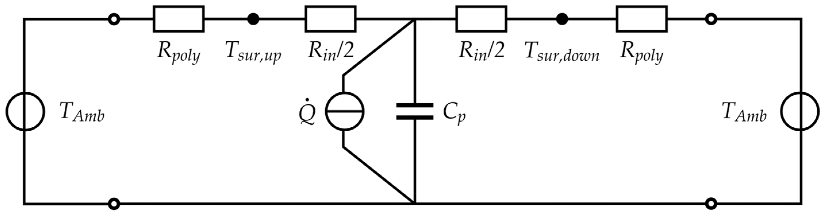
Figure 6.
Reference testing scheme. (a) Depiction of the used setup; (b) resulting temperature difference of the cell on a logarithmic scale, showing both measured and fitted data.
Figure 6.
Reference testing scheme. (a) Depiction of the used setup; (b) resulting temperature difference of the cell on a logarithmic scale, showing both measured and fitted data.
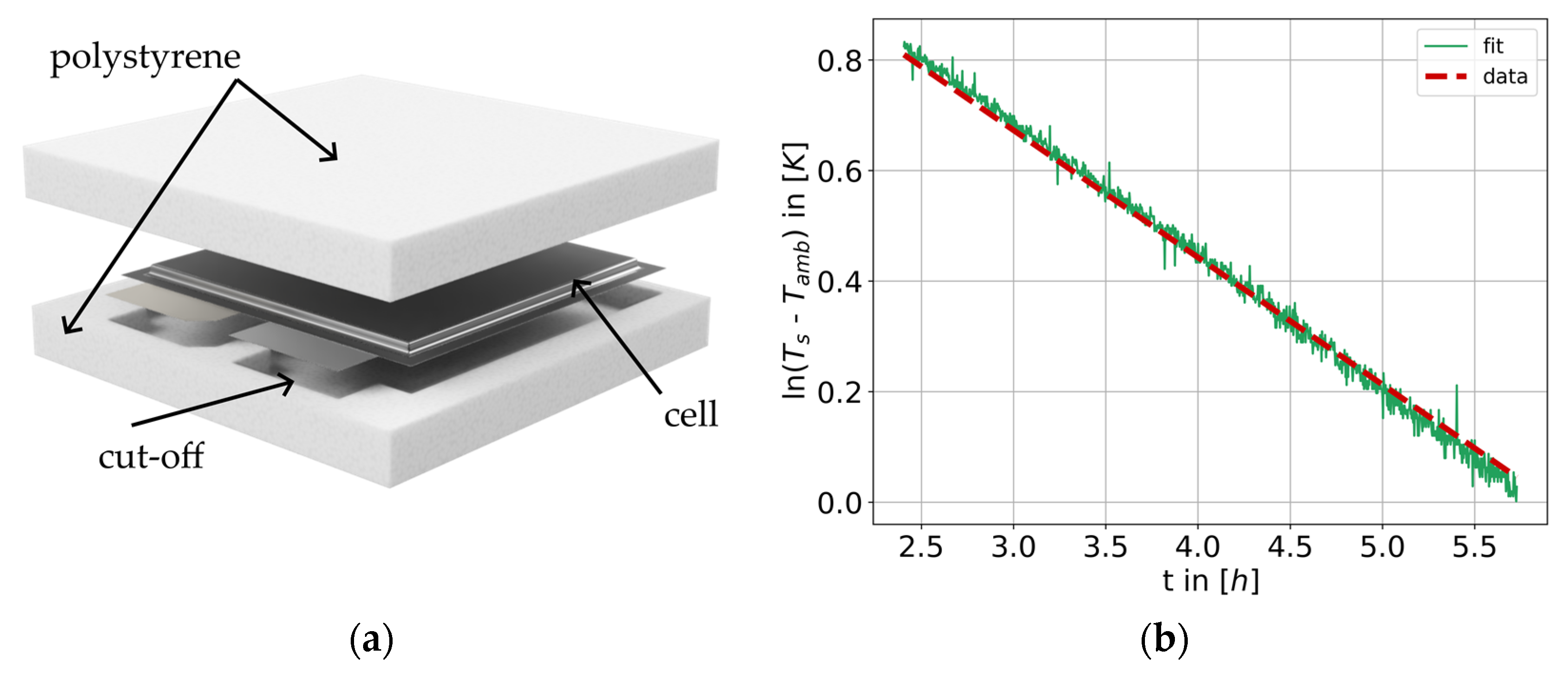
Figure 7.
Symmetry of the test setup on the top and bottom types at the same conditions (Tamb = 25 °C, SOC = 50% and I ≙ 2C).
Figure 7.
Symmetry of the test setup on the top and bottom types at the same conditions (Tamb = 25 °C, SOC = 50% and I ≙ 2C).
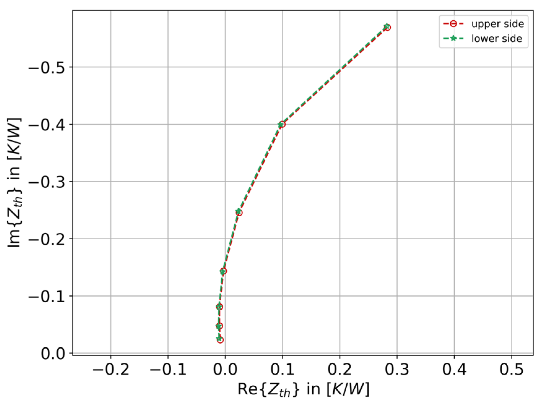
Figure 8.
Comparison of two tests using a different lower boundary frequency. (a) Nyquist plot; (b) corresponding Bode plot; top: amplitude; bottom: phase.
Figure 8.
Comparison of two tests using a different lower boundary frequency. (a) Nyquist plot; (b) corresponding Bode plot; top: amplitude; bottom: phase.

Figure 9.
Comparison of the Nyquist plot for different cell types at the same conditions (Tamb = 25 °C, SOC = 50% and I ≙ 2C).
Figure 9.
Comparison of the Nyquist plot for different cell types at the same conditions (Tamb = 25 °C, SOC = 50% and I ≙ 2C).
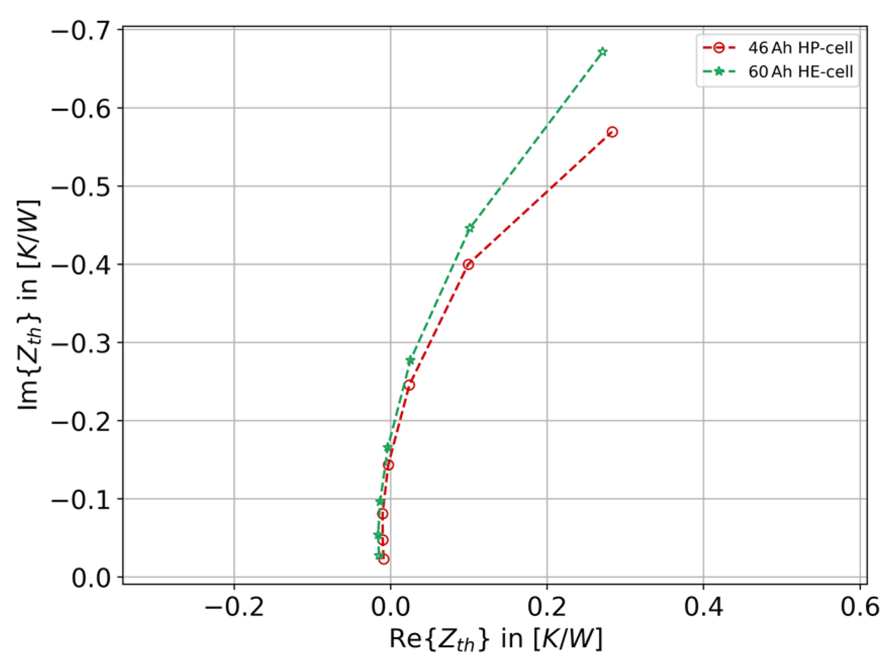
Figure 10.
Comparison of the Nyquist plot when changing a test parameter: (a) adapting SOC value using 25 °C; (b) adapting temperature using SOC at 50%.
Figure 10.
Comparison of the Nyquist plot when changing a test parameter: (a) adapting SOC value using 25 °C; (b) adapting temperature using SOC at 50%.
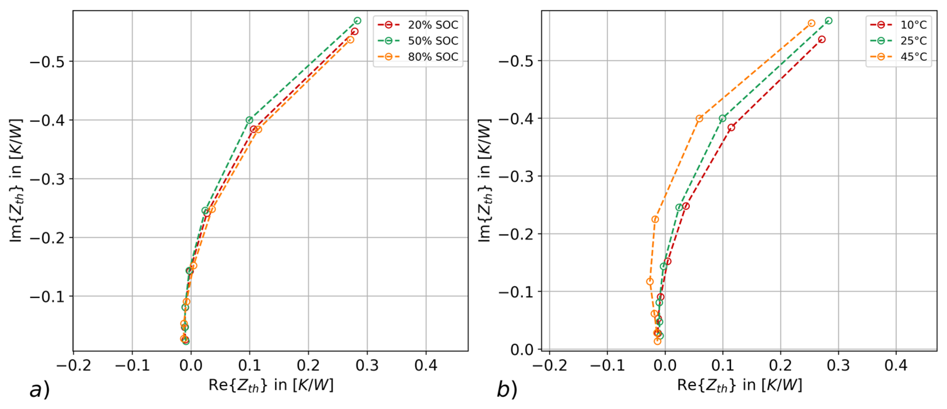
Figure 11.
Comparison of calculated data points and the resulting model fit. (a) Nyquist plot. (b) Representation of first-order Cauer model (top) and second-order Cauer model (bottom).
Figure 11.
Comparison of calculated data points and the resulting model fit. (a) Nyquist plot. (b) Representation of first-order Cauer model (top) and second-order Cauer model (bottom).
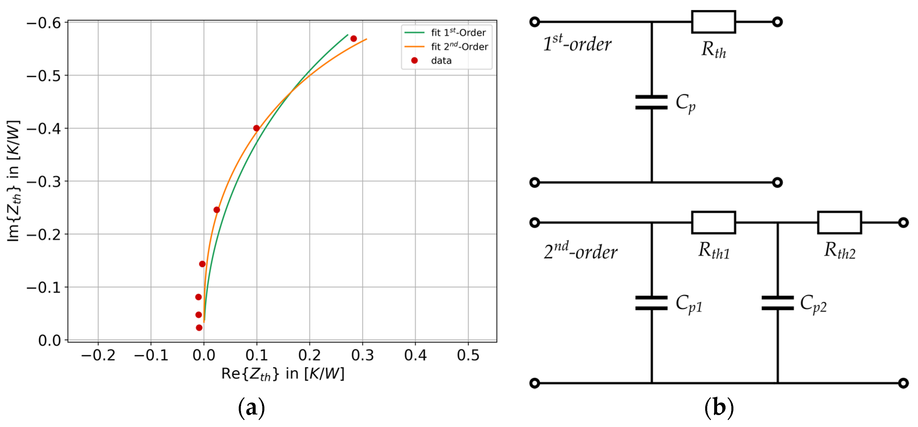
Figure 12.
Changing of thermal parameters over SOC range for all covered temperatures. (a) Specific heat capacity cp. (b) Cross-plane thermal conductivity λ⊥.
Figure 12.
Changing of thermal parameters over SOC range for all covered temperatures. (a) Specific heat capacity cp. (b) Cross-plane thermal conductivity λ⊥.
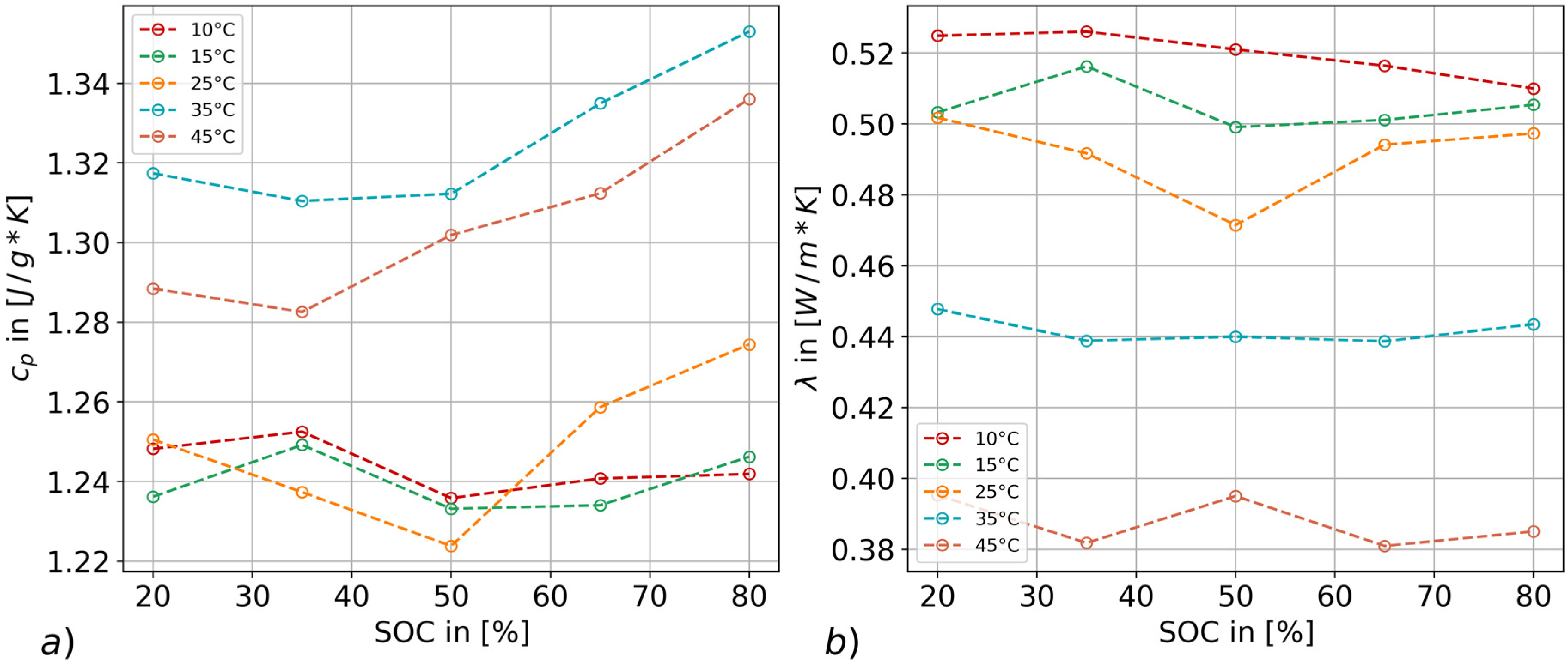
Figure 13.
Development of cross-plane thermal conductivity λ⊥ over temperature for all covered SOC. (a) Measurement points and the average at every data point. (b) Average at every data point and corresponding linear fit.
Figure 13.
Development of cross-plane thermal conductivity λ⊥ over temperature for all covered SOC. (a) Measurement points and the average at every data point. (b) Average at every data point and corresponding linear fit.

Table 1.
Signal configuration per test cycle to acquire the significant spectra.
| Frequency [mHz] | 3 | 1.8 | 1.1 | 0.7 | 0.43 | 0.26 | 0.16 |
| Repetitions [-] | 40 + 10 | 10 | 10 | 4 | 4 | 4 | 4 |
Table 2.
Resulting data for the 46 Ah and the 60 Ah cell at Tamb = 25 °C and SOC = 50%.
| 46 Ah HP Cell | 60 Ah HE Cell | |
|---|---|---|
| Time constant τ [s] | 2092 | 2312 |
| Thermal conductivity [W/(m·K)] | 0.47 | 0.40 |
| Specific heat capacity cp [J/(g·K)] | 1.25 | 1.09 |
| Specific heat capacity reference test cp [J/(g·K)] | 1.23 | 1.19 |
Disclaimer/Publisher’s Note: The statements, opinions and data contained in all publications are solely those of the individual author(s) and contributor(s) and not of MDPI and/or the editor(s). MDPI and/or the editor(s) disclaim responsibility for any injury to people or property resulting from any ideas, methods, instructions or products referred to in the content. |
© 2023 by the authors. Licensee MDPI, Basel, Switzerland. This article is an open access article distributed under the terms and conditions of the Creative Commons Attribution (CC BY) license (https://creativecommons.org/licenses/by/4.0/).
Share and Cite
MDPI and ACS Style
Droese, D.; Kowal, J. Thermal Characterisation of Automotive-Sized Lithium-Ion Pouch Cells Using Thermal Impedance Spectroscopy. Appl. Sci. 2023, 13, 2870. https://doi.org/10.3390/app13052870
AMA Style
Droese D, Kowal J. Thermal Characterisation of Automotive-Sized Lithium-Ion Pouch Cells Using Thermal Impedance Spectroscopy. Applied Sciences. 2023; 13(5):2870. https://doi.org/10.3390/app13052870
Chicago/Turabian StyleDroese, Dominik, and Julia Kowal. 2023. "Thermal Characterisation of Automotive-Sized Lithium-Ion Pouch Cells Using Thermal Impedance Spectroscopy" Applied Sciences 13, no. 5: 2870. https://doi.org/10.3390/app13052870
Note that from the first issue of 2016, this journal uses article numbers instead of page numbers. See further details here.