

An Open-Source Software Reliability Model Considering Learning Factors and Stochastically Introduced Faults
1
School of Automation and Software Engineering, Shanxi University, Taiyuan 030006, China
2
School of Computer Science and Technology, Harbin Institute of Technology at Weihai, Weihai 264209, China
*
Author to whom correspondence should be addressed.
Appl. Sci. 2024, 14(2), 708; https://doi.org/10.3390/app14020708
Submission received: 2 December 2023
/
Revised: 6 January 2024
/
Accepted: 10 January 2024
/
Published: 14 January 2024
(This article belongs to the Topic Software Engineering and Applications)
Abstract
:In recent years, software development models have undergone changes. In order to meet user needs and functional changes, open-source software continuously improves its software quality through successive releases. Due to the iterative development process of open-source software, open-source software testing also requires continuous learning to understand the changes in the software. Therefore, the fault detection process of open-source software involves a learning process. Additionally, the complexity and uncertainty of the open-source software development process also lead to stochastically introduced faults when troubleshooting in the open-source software debugging process. Considering the phenomenon of learning factors and the random introduction of faults during the testing process of open-source software, this paper proposes a reliability modeling method for open-source software that considers learning factors and the random introduction of faults. Least square estimation and maximal likelihood estimation are used to determine the model parameters. Four fault data sets from Apache open-source software projects are used to compare the model performances. Experimental results indicate that the proposed model is superior to other models. The proposed model can accurately predict the number of remaining faults in the open-source software and be used for actual open-source software reliability evaluation.
1. Introduction
Over the past couple of decades, OSS has developed rapidly through the development of Internet technology. The way that OSS is developed is completely different to traditional CSS, which is hierarchical, closed, and centrally managed and developed. The development and testing of CSS is the responsibility of dedicated staff and completed according to a plan with clear tasks and responsibilities. Once CSS testing is completed and delivered, it is difficult to presently implement the new feature and requirement changes in the software in the software’s current version. If there is a failure in the subsequent delivery, there is a need to spend a lot of manpower and capital to maintain and repair the failure. However, the OSS development method is more flexible and changeable. Raymond [1] referred to CSS and OSS development methodologies as the cathedral and bazaar, respectively.
Compared to traditional CSS development, OSS is developed and tested by volunteers and users around the world through the network. OSS is developed in a dynamic, uncertain, networked, and distributed environment. OSS development does not require centralized management, there is no clear leader, and it is completely completed by contributors including developers, volunteers, and users. In general, volunteers and users are paid nothing to develop and test OSS. They develop and test the functionality of OSS and are completely driven by interest and hobbies. Raymond [1] also pointed out that in the process of OSS development, as long as enough effort is made, all bugs can be detected. However, due to the current development environment and conditions, bugs in OSS cannot be fully detected, and there will be some remaining vulnerabilities in the new version of an OSS.
Modern well-known companies and businesses have OSS development projects. Examples include Google, Microsoft, and Alibaba. In particular, some big data and cloud computing application systems are developed and tested in an open-source manner. Although OSS development is widely used in the industry, its reliability remains a concern.
To improve the reliability of OSS, the industry generally adopts the method of frequent release [1]. Although the frequent release of OSS can improve the reliability to some extent, there are some problems with this simple method of frequent release. First, if the release of OSS occurs too early, the software is not fully tested and there are too many vulnerabilities left in the software. They will influence the user experience of volunteers and users and force volunteers and users to not use the software but to find alternative software. Second, if the software is not released on time, it will miss the opportunity. Volunteers and users will get disinterested in the software, while other OSSs will be used and developed by volunteers and users instead of the software in question.
In order to assess the reliability of OSS, there are some RMs in the literature [2,3,4,5,6,7,8,9,10,11,12]. For example, Li et al. [2] proposed an RM of OSS with a first increasing and then decreasing FDR. By studying OSS fault data sets, Wang and Mi [3] developed an OSS RM with a decreasing trend of FDR. Zhou and Davis [4] concluded that CSS RMs can be used to assess the reliability of OSS through some experiments. Yamada and Tamura established a few RMs for OSS based on SDEs [8,9,10,11]. The above models are all perfect debugging software RMs. Specifically, this means that the removal of an identified fault should not result in the introduction of any NFs. The assumption of perfect debugging is not in line with the actual situation of OSS development.
On the other hand, in order to satisfy user demands and gradually improve product functions, OSS is generally multi-version release software. Through the continuous modification of each version of the software, the developed OSS projects gradually meet the needs of users. OSS will modify and improve some features and functionality of the original version after each release of a new version. In the new version, some additional functions are added, and useless functions are reduced. Therefore, OSS will add some additional vulnerabilities in the new version. The elimination of these faults may result in the introduction of NFs. This can be seen from the bug report in bug tracking systems. In bug tracking systems, we can see that the fault types of OSSs have New Feature, Improve, Bug, etc. Among them, New Feature and Improve are types of newly introduced faults. In bug tracking systems, we can see that the status of an OSS includes OPEN, REOPENED, IN PROGRESS, CLOSED, etc. When the status of the fault of an OSS is reopened, it means that the fixed fault needs to be removed again due to incomplete removal or the introduction of a new fault.
From the above analysis, it can be concluded that there are two ways to introduce faults in an OSS. One is to bring in some faults when the functions of the new version of the OSS change, and NFs appear when these faults are eliminated. Second, when the remaining faults in the original version are removed, new introduced faults are added into the new version. Due to the continuous changes in and modifications of OSS in the development process, the imported fault behavior is uncertain. The introduction of the fault is irregular and a kind of random change.
In addition, OSS is an iterative development approach that continuously modifies and releases new versions of the software to meet user and actual functional needs. Community contributors understand the improvement in software functionality and the addition of new features through continuous use and learning. Therefore, software testers go through a learning process for OSS, and they fully understand the changes in the software through continuous learning. Usually, the cumulative number of faults detected will show an S-shaped curve change with the testing time.
In this study, we propose an OSS RM considering learning factors and SIFs. Note that the introduction of faults here includes three aspects. First, NFs can arise when faults caused by software changes are removed. For example, modifications are made to software features, functionality, or modules subsequent to the release of the most recent OSS version. Second, NFs are introduced when the remaining faults which are detected in the previous software version are removed. Third, two introduced faults are cascading or correlated (or more specifically, one fault introduced simultaneously by two types). For instance, when a new function (e.g., storage) is introduced. Meanwhile, the new change corrects some previous faults in the data structure. There is a chance that a fault appears due to both factors. In other words, we classify Type V faults as faults that are related to version changes, Type R faults as faults that are related to a previous fault removal, and Type S faults as faults that are related to Type V and Type R faults. For the rest of the paper, these three types (V, R, and S) can be used as references.
Therefore, we propose that the OSS RM, considering the random change in the fault introduction, can be effectively applied in the actual evaluation of OSS reliability. In addition, stochastic equations are used to simulate irregular changes in the introduction of faults. The PM is established in the OSS development environment and is more consistent with the actual legal changes of introduced faults. The PM can help developers and managers evaluate the reliability of an OSS and guide the optimal release of an OSS.
The contributions of this paper are as follows:
- (1)
- We propose that in the processes of OSS development, testing, and debugging, fault introduction has the characteristics of stochastic changes.
- (2)
- We use SDE to simulate the stochastic change of three types of fault introductions in the processes of OSS development, testing, and debugging.
- (3)
- We propose that in the processes of OSS development, testing, and debugging, fault introduction is related to existing faults in the software.
Considering that fault removal during OSS debugging is influenced by the skills, mindset, environment, resources, and tools of the debugging personnel, it is possible to introduce faults when removing them, and the introduction of faults is randomly changing. In other words, if the introduced faults are not randomly changing but are introduced in a regular manner, then in the actual process of fault removal, fault introduction can be completely avoided. The reality is that debugging personnel have no idea and cannot predict in advance when, where, in which module or function, and how many faults will be introduced. This means that fault introduction in OSSs occurs randomly.
The remainder of the paper is structured as follows:
Related work is introduced in Section 2. In Section 3, the development process of the PM is presented in detail. Section 4 introduces fault data sets, model comparison criteria, and the model parameter estimation method. The performance comparison experiments of models are conducted in Section 4. The sensitivity analysis is discussed in Section 5. Section 6 presents threats to the validity of the PM. Conclusions are summarized in the final section.
2. Related Work
Generally speaking, OSS is dynamically developed multi-release software. It will release new functional software as development requirements change. Considering the characteristics of OSS’s dynamic development, we can establish two types of OSS RMs to evaluate software reliability. One is to assume that the faults in a continuously released OSS are irrelevant and establish a single-release OSS RM. The second is to assume that there are correlations between faults in successive releases of OSS, so as to establish the corresponding multi-release OSS RM.
The single-release OSS RM can evaluate the reliability of each version of an OSS without considering the fault correlation in each version. For example, Lin and Lin [13] proposed an OSS RM based on a rate queue theory. To solve the problem of delay in FD and the elimination of OSS, considering that the FD process of OSS obeys a Pareto distribution, Huang et al. [14] proposed an RM of OSS considering the bounded generalized Pareto distribution. By studying the early FD process for OSS, Lee [15] proposed a method to predict the reliability of OSS. Through a systematic study of the OSS development process, Yamada and Tamura [16] proposed a reliability measurement and evaluation methods of OSS.
Through extensive research on OSS projects, Miko et al. [17] have pointed out that traditional CSS RMs can be used for the reliability assessment of OSS projects. But no software RM can be applied to all OSS development and testing environments. Considering the remnant faults from the previous version and faults generated by changes in software functions, features, and components in the newly released version of an OSS, Zhu and Pham [18] established the RM of OSS. Wang [19,20] proposed two OSS RMs. One considered that the introduction of faults followed a Pareto distribution, and the other considered that FD and fault introduction changed nonlinearly over time. Huang et al. [21] proposed an ID software RM that considers the decreasing fault fluctuation rate function. Considering the factors of learning and tester fatigue during software testing, Yaghoobi and Leung [22] proposed a software RM based on learning and fatigue factors. Considering the different issue types in the issue tracking system, Singh et al. [23] proposed two different software RMs to evaluate the reliability of OSS. Singhal et al. [24] proposed two software RMs that consider stochastic debugging for OSS. Considering the importance of test coverage in software testing, Singhal et al. [24] proposed two software reliability models: a perfect debugging model based on fault removal efficiency, and an imperfect debugging model based on operating environment uncertainty. Liu and Xie [25] proposed a new software RM based on a gray system theory and validated the effectiveness of the PM through experiments. Jagtap [26] proposed a hybrid nonparametric method to predict software faults and evaluate software reliability.
In addition, Garg et al. [27] proposed a hybrid method to select the optimal software RM, as no software RM can demonstrate optimal reliability evaluation performance in all software testing environments. Singh et al. [28] presented a method to select the optimal software RMs based on integrating CRITIC and CODAS. Considering the significant correlation between software RMs and fault data sets, the optimal software RM should be selected for the current software reliability evaluation. Yaghoobi [29] proposed two methods to select the current optimal software RM.
On the other hand, a multi-release OSS RM can assess the reliability of each version of an OSS considering the fault correlation in each version. For example, Yang et al. [30] proposed RMs of OSS that consider delays between FD and fault removal. Saraf et al. [31] proposed a general multi-release software framework with FD and correction considering the ID and changing point. Khurshid et al. [32] also proposed a multi-release OSS RM considering the changing point and ID. Considering the change in source code files of OSS, Singh et al. [33] proposed an entropy-based multi-release RM of OSS. In addition, considering fault dependence in multi-release open-source software, Chatterjee et al. [34] proposed an RM with an ID and changing point. By studying fault introduction phenomena of OSS, Gandhi et al. [35] established a corresponding RM. Diwakar and Aggarwal [36] proposed an RM for OSS that considers ID. By studying changes in fault-decreasing factors and testing coverage, Tandon et al. [37] built a multi-release RM for OSS. Saraf et al. [38] proposed an integrated method to build a multi-release OSS RM based on a variety of testing and debugging environments. Pradhan et al. [39] proposed two single-release software RMs and one multi-release software RM while considering the fault reduction factor with a generalized inflection S-shaped distribution.
In order to optimize the parameter estimation of OSS RMs, Yang et al. [40,41] used the expectation maximization algorithm to compute the likelihood function of software RMs. Additionally, Yang et al. [42] used the expectation least squares and expectation maximization algorithms to estimate OSS RM parameters while considering the processes of FD and correction. Xiao et al. [43] used an artificial neutral network to build a software RM and predicted the number of the software’s remaining faults while considering FD, correction, and testing efforts. Considering the problem of resource allocation in the process of software testing, a multi-objective optimization approach was put forth by Rani and Mahapatra [44] to address the issue of allocating resources for software testing.
In the above-mentioned OSS RMs, although some models consider the random change in FD, they do not consider the random change introduced by faults. Moreover, fault introduction in OSSs includes not only the fault introduced during debugging, but also the new fault introduced when faults from the changes in software functions, features, and components are removed following the release of the new OSS version. Therefore, the introduced faults show irregular changes. In other words, in the OSS testing and debugging processes, the behavior of introducing faults is random. In this paper, we use SDE to simulate the random change in fault introduction, which is more consistent with the actual situation of fault introduction in the processes of OSS testing and debugging.
3. Modeling Fault Introduction Process
A fault introduction in an OSS includes three aspects (i.e., Types V, R, and S). Type V is the introduced faults in the new version of software due to changes in the function, features, and components of OSS. Type R is a fault introduced in the process of the troubleshooting of the remaining faults from the previous version. Type S is a fault introduced simultaneously by the previous two types. The three kinds of introduced faults show irregular changes in OSS fault reports, and the behavior of the introduced faults is uncertain. Thus, fault introduction is random during the development of an OSS. Considering that the number of faults introduced in () is related to the software fault itself, we give the following differential equation:
where represents the fault content function, which is a total number of fault counts in the testing process of a single version of an OSS. denotes the intensity function of the software fault introduction. It represents the change in the fault introduction and is a non-negative value. a represents the expected total number of initially detected faults. The effort spent on debugging can speed up the number of faults that are detected, but a is the constant, and the total number is certain.
In Equation (1), is the intensity of software introduction faults. is the not the fault density. Herein, the intensity of software introduction faults refers to the number of introduced faults and is increasing cumulatively, or at least not decreasing. The intensity value of the software introduction faults can be greater than one.
Because the number of introduced faults is uncertain in the process of OSS testing and debugging, fault introduction is random, and the fault introduction intensity function shows irregular changes. Equation (1) can be extended to the following SDE [45,46].
where represents a standardized white noise of Gaussian. denotes a magnitude of the irregular fluctuation and is a positive constant value. The reasons for with Gaussian distribution are presented below.
Considering the complexity of fault introduction in OSS, we establish differential Equation (1). In order to improve Equation (1), we add irregular fluctuation (please see Equation (2)) to the fault introduction intensity function due to the random variation in introduced faults during the debugging process of OSS. Herein, “intensity” of fault introduction (always positive or equal to 0) means that the number of introduced faults is increasing cumulatively, or at least not decreasing. This is consistent with the cumulative increase in the number of faults that are introduced in the debugging process of OSS.
When OSS is released, the effect of noise affecting the introduction of faults will gradually increase due to the uncertainty of the software debugging environment, debugging tools, debugging personnel, and skills. For a period of time after the release of an OSS, debuggers gradually become familiar with and understand the software through continuous learning, testing, and debugging. The effect of noise that affects the introduction of faults will gradually decrease. Especially, due to the small number of faults detected at the later stage of testing, the number of introduced faults is gradually reduced. The effect of noise that affects the introduction of faults has weakened, so it is a normal distribution.
Solving the SDE of type in Equation (2), we can derive as follows:
where and d represent a rate parameter of the intensity of fault introduction and a shape parameter, respectively.
In addition, we assume that the number of faults discovered instantaneously is related to the number of remaining faults in the software [47], and FD obeys an NHPP. We also consider learning phenomena during FD. Thus, the following differential equation can be derived:
Substituting Equation (3) into Equation (4),
where is the mean value function representing the expected cumulative number of the detected faults by time t. b(t) denotes an FDR function, and . b represents an FDR and is an IF. b(t) shows an S-shaped curve change over time.
Note that we propose three types of introduced faults to illustrate the phenomenon of fault introduction and the random changes in the debugging process of OSS. We assume that the number of faults detected instantaneously is related to the remaining number of faults in the software, where “instantaneous” refers to the number of faults that are detected in (), which is related to the number of remaining faults in the software.
In this paper, we consider that there is a learning process for OSS during FD. In other words, the learning phenomenon occurs during software testing, where software testers go through a learning process. Herein, software testers refers to software developers, volunteers in the community, or members in the team. This learning process presents an S-shaped curve with the cumulative number of detected faults over the testing time.
Assuming that the intensity function of the fault introduction obeys the Weibull distribution, the reason is that the shape parameter of the Weibull distribution is flexible. By changing the shape parameter of the Weibull distribution, a variety of fault data changes can be simulated. Therefore, the Weibull distribution can simulate the complex process of fault introduction for OSS.
Equation (5) is an expression of the PM. It should be noted that in order to simplify the modeling calculation, a Taylor formula expansion and truncation are used in the process of model derivation. Please refer to Appendix A for a detailed model derivation process.
We consider that the newly generated faults in the current version are only related to the new functional changes in the current version and have nothing to do with the remaining faults in the previous version. Furthermore, the related research indicated that faults in the current version are not related to the faults in the previous version in most cases for OSS [48].
Note that the case of fault masking [49] is considered to detect faults rather than introduce new ones in this study. In addition, the work of this paper focuses on the establishment of the RM of OSS, which is used to evaluate the reliability of OSS. In order to avoid ambiguity, we call the PM an OSS RM rather than an OSS fault model.
In this paper, software reliability refers to the probability that software runs without faults for a certain amount of time in a given environment. Assuming that the FD follows an NHPP, software reliability can be expressed as follows:
In Equation (6), within a time interval of [t, t + x], the process of software failure follows the NHPP. This is the mathematical expression formula for software reliability. Among them, represents the MVF; in other words, it denotes the expected cumulative number of faults detected by time t. is also called software RM.
4. Numerical Examples
4.1. Fault Data Sets for OSS
The fault data sets used in this paper are collected from four projects of Apache OSS products (https://issues.apache.org/jira/issues, accessed on 5 January 2023), KNOX, NIFI, TEZ, and BIGTOP. Each project of OSS has three successive versions. The first fault data set (DS1), collected from the KNOX project of Apache OSS products, has three subsets, KNOX 0.3.0 (DS1-1), KNOX 0.4.0 (DS1-2), and KNOX 0.5.0 (DS1-3). The second fault data set, collected from the NIFI project of Apache OSS products, has three subsets, NIFI 1.2.0 (DS2-1), NIFI 1.3.0 (DS2-2), and NIFI 1.4.0 (DS2-3). The third fault data set, collected from the TEZ project of Apache OSS products, has three subsets, TEZ 0.2.0 (DS3-1), TEZ 0.3.0 (DS3-2), and TEZ 0.4.0 (DS3-3). The fourth fault data set (DS) was obtained from the BIGTOP project of Apache OSS products. These fault data sets include three successive software versions: BIGTOP 0.3.0 (DS4-1) from October 2011 to April 2012, BIGTOP 0.4.0 (DS4-2) from September 2011 to October 2012, and BIGTOP 0.5.0 (DS4-3) from September 2011 to December 2012.
Note that the attributes of the faults in bug tracking systems include Type, Status, Resolution, etc. The type of fault data collected by us include all standard issue types and all substandard issue types. The fault data status includes OPEN, INPROGRESS, REOPENED, RESOLVED, AND CLOSED. The fault data resolution excludes Duplicate, Invalid, Not A Problem, Cannot Reproduce, and Not A Bug. Table 1 lists the detailed information on the fault data sets that are used in this paper. Table 2 shows all software RMs for comparison. In Table 2, there are six CSS RMs, the G-O model, the Delayed S-shaped model, the Inflection S-shaped model, the Yamada Imperfect-2 model, the P-N-Z model, and the Weibull distribution model, and three OSS RMs, the Wang model, the Li model, and the PM.
In this paper, we collected fault data sets using time (days or weeks) in the bug tracking system (please see Table 1). We used the collected fault data sets to fit and estimate the model parameters’ values. We can predict the number of faults in a software using the model. Thus, graphs in the paper depict the evolution across time (days or weeks).
Although the fault data set used in this experiment is relatively old, using it to evaluate and validate the performance of the model still has practical reference value and guiding significance for modern software testing. Although modern software development methods, languages, and processes have undergone many changes, in the actual software testing process, most modern OSSs also follow the same rules as previous open-source software testing did. The model that we propose is entirely based on the study of the phenomenon of random changes introduced by faults during software debugging. Therefore, the RMs developed based on these data sets still have important practical reference value and practical guidance significance for modern OSS testing.
4.2. Model Comparison Criteria
In this paper, the performance of models is evaluated using six model comparison criteria:
- Mean Square Error (MSE) [55]. This metric is used to assess how well software RMs fit and predict performance. It calculates the deviation between the estimated fault number of a software RM and the actual fault number detected during software testing.and
- Root Mean Square Error (RMSE) [55]. This measures the square root of the distance between the estimated values and the actual observations. In general, it is used to evaluate the fitting and predictive performance of software RMs.and
- Kolmogorov–Smirnov test (K-S test) [56]. This metric is intended to assess how well software RMs fit. At every point, it calculates the absolute deviation between the expected distribution function from the model and the normalized cumulative distributions of the actual observed rates.Equation (12) is also called Kolmogorov distance (KD).Di = supy|Fi(y) − F(y)|
- The Theil statistic (TS) [55]. This is the average distance percentage between the estimated values from the model and the actual values.and
- Bias [55]. This is the sum of the deviation between the observed values and the estimated values from the model.and
In Equations (7)–(16), denotes the estimated number of faults detected by time . represents the number of faults observed by time . n and m are the sample size of the fault data. In Equations (8), (11), (14), and (16), the first (n-m) fault times are used to estimate the model parameter values, and the remaining fault times are used to compute the prediction values. Note that the smaller the MSE (MSEpredict), Dk, RMSE (RMSEpredict), TS (TSpredict), and Bias (Biaspredict) values are, the better the predictive or fitting performance of the model is. The larger the value of R2 is, the better the model’s fitting ability is.
4.3. Estimating Model Parameters
LSE was used in this paper to estimate the model’s parameter values. In general, MLE can be used to estimate the parameter values of a model in software reliability modeling. The error utilizing LSE and MLE to estimate model parameter values is quite tiny, because the fault data sets have a small sample size. Furthermore, the value of the maximum likelihood function may not exist in some scenarios [57]. The LSE method can be presented as follows:
where represents the estimated number of faults detected by time . denotes that the number of faults observed by time . Equation (17) takes partial differential equations on both sides.
Solving Equations (18)–(23), we can calculate the estimated values of the model parameters (a, b, , , d, and ). Additionally, the MLE function of the PM can be denoted as follows:
Take the logarithm on both sides of Equation (24).
The partial differential equation for Equation (25) can be obtained as follows (Equation (26)):
We can obtain the estimated parameter values (a, b, ,, d, and ) of the PM by solving Equation (26). Notably, the values of the maximum likelihood function may not exist when MLE is used to estimate the model parameter values [57].
4.4. Analysis and Discussion of Model Performance Comparison Using LSE Estimation Parameter Values
In terms of fitting, model parameter values are fitted and estimated using 100% of the fault data, and the model fitting performances are compared. In terms of prediction, the model parameter values are fitted and estimated using 85% of the fault data, and we use the residual fault data (15% of the fault data) to compare the models’ predictive performance.
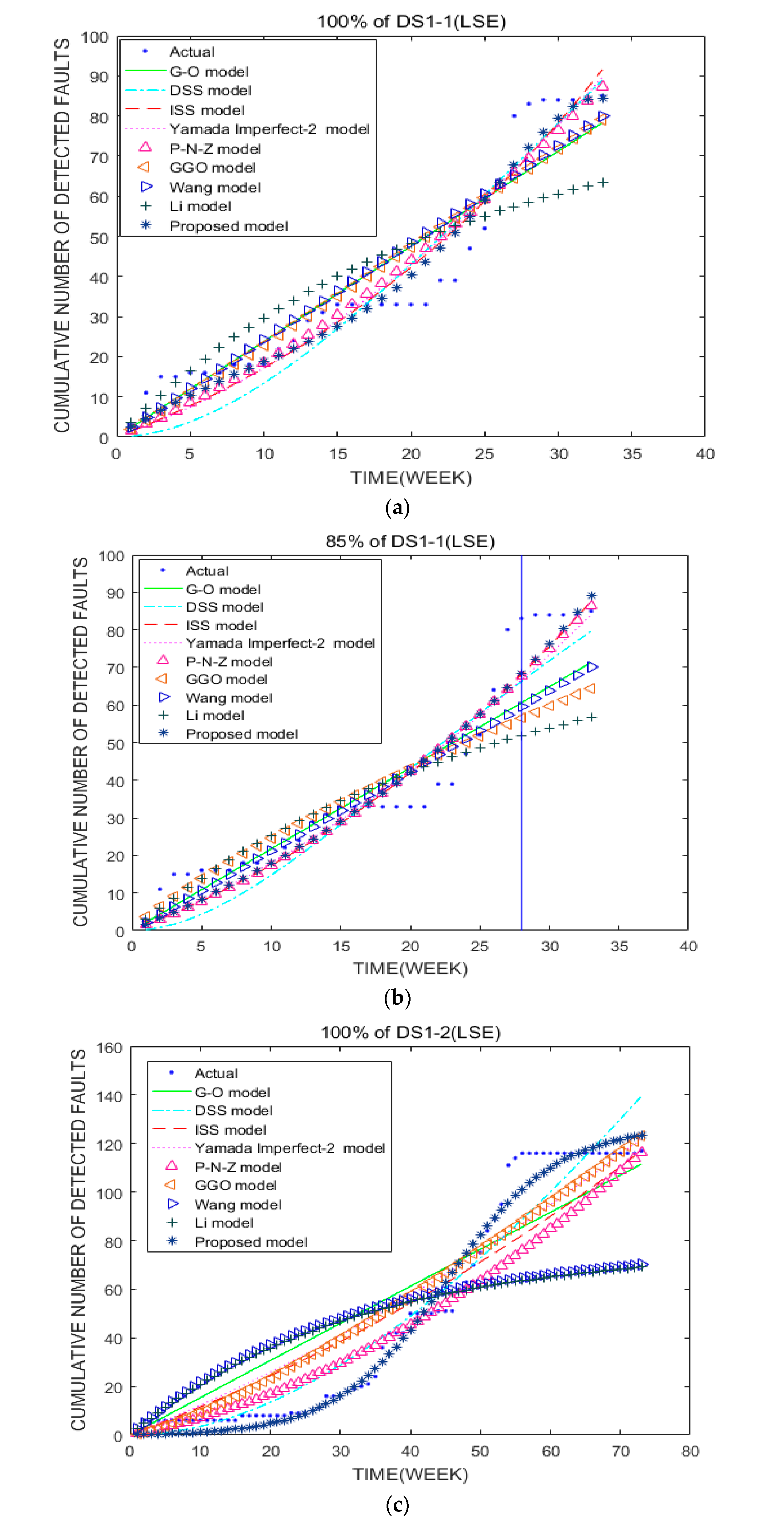
From Table 3, Table 4 and Table 5, we can see that using 100% of the data (DS1-1, DS1-2, and DS1-3), the MSE, R2, RMSE, KD, TS, and Bias values of the PM are 35.85, 0.9456, 5.99, 0.1438, 12.68, and 4.82; 39.4, 0.9809, 6.28, 0.1762, 9.22, and 4.99; and 16.02, 0.9554, 4.0, 0.1732, 13.25, and 3.67, respectively. In Table 3, the MSE, RMSE, TS, and Bias values of the ISS model which ranked second are approximately 1.45, 1.21, 1.21, and 1.28 times as large as those of the PM, respectively. In Table 4, we can see that the MSE, RMSE, TS, and Bias values of the DSS model which ranked second are nearly 2.85, 1.78, 1.28, and 1.73 times as large as those of the PM, respectively. Table 5 shows that the MSE, RMSE, and TS values of the DSS model which ranked second are about 1.64, 1.28, and 1.28 times as large as those of the PM, respectively. The PM outperforms the G-O model, DSS model, ISS model, Yamada Imperfect-2 model, P-N-Z model, GGO model, Wang model, and Li model in terms of fitting performance. Using 100% of the data (DS1-1, DS1-2, and DS1-3), the second best is the ISS model run once and the DSS model run twice. The worst is the Li model, which is three times worse in its ranking. These results can be seen in Figure 1a,c,e.
Table 6, Table 7 and Table 8 show that using 100% of the data (DS2-1, DS2-2, and DS2-3), the MSE, R2, RMSE, KD, TS, and Bias values of the PM are 1040, 0.9619, 32.25, 0.2497, 14.95, and 22.76; 356.92, 0.8562, 18.89, 0.3842, 29.18, and 12.93; and 1142.3, 0.7558, 33.8, 0.392, 40.18, and 27.67, respectively. According to Table 6, the MSE, RMSE, TS, and Bias values of the second-placed GGO model are roughly 0.45, 0.53, 0.54, and 0.58 times higher than those of the PM, respectively. In Table 7, we can see that the MSE, RMSE, TS, and Bias values of the DSS model which ranked second are about 1.33, 1.16, 1.15, and 1.33 times as large as those of the PM, respectively. The performance of fitting is the highest for the PM. Using 100% of the data (DS2-1, DS2-2, and DS2-3), the second best is the GGO model, and then, the DSS model and the P-N-Z model, respectively, follow. The worst is the Li model, which is three times worse in terms of its ranking. Figure 2a,c,e show the fitting comparison of the models.
Table 9, Table 10 and Table 11 show that using 100% of the data (DS3-1, DS3-2, and DS3-3), the MSE, R2, RMSE, KD, TS, and Bias values of the PM are 122.31, 0.9907, 11.06, 0.0741, 4.54, and 8.47; 113.84, 0.9053, 0.67, 0.2245, 25.73, and 8.02; and 57.79, 0.804, 7.6, 0.3472, 38.08, and 5.42, respectively. From Table 9, we can see that the MSE, RMSE, TS, and Bias values of the second-placed G-O model are almost 1.23, 0.5, 0.5, and 0.62 times more than those of the PM, respectively. Table 10 shows that the MSE, RMSE, KD, TS, and Bias values of the second-placed P-N-Z model are around 1.3, 0.52, 0.57, 0.52, and 0.6 times larger than those of the PM, respectively. The PM has the best fitting performance of all the models. Using 100% of the data (DS3-1, DS3-2, and DS3-3), the next-best performing models are the G-O model, the P-N-Z model, and the ISS model, respectively. The worst is the Li model when run once and the Wang model when run twice. From Figure 3a,c,e, we can see the fitting comparison of models.
From Table 12, Table 13 and Table 14, we can see that using 85% of the data (DS1-1, DS1-2, and DS1-3), the MSEprdict, RMSEprdict, TSprdict, and Biasprdict values of the PM are 45.63, 6.76, 8.02, and 0.84; 211.38, 14.54, 12.52, and 2.05; and 113.91, 10.67, 17.21, and 1.22, respectively. In Table 12, the MSEprdict, RMSEprdict, and Biasprdict values of the ISS model which ranked second are approximately 1.09, 1.04, and 1.02 times as large as those of the PM, respectively. Table 13 shows that the MSEprdict, RMSEprdict, and Biasprdict values of the G-O model, which came in second place, are 0.82, 0.35, and 0.4 times higher than those of the PM, respectively. Table 14 reveals that the MSEprdict, RMSEprdict, and Biasprdict values of the second-placed DSS model are approximately 1.92, 0.71, and 0.91 times greater than those of the PM, respectively. The PM outperforms the G-O model, DSS model, ISS model, Yamada Imperfect-2 model, P-N-Z model, GGO model, Wang model, and Li model in terms of prediction performance. The second best is the ISS model and the worst is the Li model. The PM outperforms the G-O model, DSS model, ISS model, Yamada Imperfect-2 model, P-N-Z model, GGO model, Wang model, and Li model in terms of fitting performance, as shown in Figure 1b.
The G-O model comes in second, while the DSS model comes in last, using 85% of the data (DS1-2). Figure 1d shows that the Yamada Imperfect 2 model has superior fitting performance compared with the other models, but the suggested model performs worse than it. However, compared to the Yamada Imperfect 2 model, the PM performs predictions more accurately. The DSS model comes in second with 85% of the data (DS1-3), and the Li model comes in last. The PM has the greatest fitting and predictive performance among them, as shown in Figure 1f.
From Table 15, Table 16 and Table 17, we can see that using 85% of the data (DS2-1, DS2-2, and DS2-3), the MSEprdict, RMSEprdict, TSprdict, and Biasprdict values of the PM are 1789.1, 42.3, 10.72, and 5.48; 92.41, 9.61, 8.74, and 1.19; and 1484.8, 38.53, 19.6, and 5.1, respectively. Comparing the PM to other models, it performs predictions more accurately. The second best is the P-N-Z model, and the worst is the Li model. According to Table 15, the MSEprdict, RMSEprdict, and Biasprdict values of the second-ranked Yamada Imperfect-2 model are around 1.16, 0.47, and 0.6 times larger than those of the PM, respectively. Table 16 shows that the MSEprdict, RMSEprdict, and Biasprdict values of the Yamada Imperfect-2 model, which came in second place, are 1.05, 0.43, and 0.42 times larger than those of the PM, respectively. Table 17 reveals that the MSEprdict, RMSEprdict, and Biasprdict values of the second-placed ISS model are approximately 3.14, 1.03, and 0.76 times greater than those of the PM, respectively. Figure 2b demonstrates the generality of the PM’s fitting performance. However, the PM performs prediction better than the other models.
The DSS model comes in second, and the Wang model comes in last, using 85% of the data (DS2-2). We can see from Figure 2d that the suggested model’s performance in terms of fitting is better than the G-O model, GGO model, Wang model, and Li model, but worse than the DSS model, ISS model, Yamada Imperfect-2 model, and P-N-Z model. Yet, the PM performs predictions more accurately than the other models. Using 85% of the data (DS2-3), the second best is the ISS model, and the worst is the Li model. Figure 2f shows that the PM’s fitting performance is better than the other models, except for the ISS model, which achieves a better performance. The PM also has the highest prediction accuracy of any of them.
Table 18, Table 19 and Table 20 show that using 85% of the data (DS3-1, DS3-2, and DS3-3), the MSEprdict, RMSEprdict, TSprdict, and Biasprdict values of the PM are 28.75, 5.36, 1.38, and 0.61; 1469.1, 38.33, 38.71, and 5.28; and 9.13, 3.02, 6.2, and 0.39, respectively. The PM has better predictive performance than the other models. The second best is the ISS model, and the worst is the Wang model. Table 20 shows that the MSEprdict, RMSEprdict, and Biasprdict values of the ISS model which ranked second are about 60.69, 6.86, and 7.26 times larger than those of the PM, respectively. From Figure 3b, we can see that the fitting and predictive performance of the PM is better than the other models’ performances. Using 85% of the data (DS3-2), the second best is the GGO model, and the worst is the Wang model. From Figure 3d, we can see that the fitting and predictive performance of the PM is better than those of the other models. Using 85% of the data (DS3-3), the second best is the ISS model, and the worst is the Wang model. Figure 3f shows that the PM outperforms other models in terms of fitting performance. Moreover, the PM has the best predictive performance among them.
In general, compared with other models, the PM has better predictive performance and better fitting performance except for when using 85% of the data (DS1-2, DS2-1, DS2-2, and DS2-3). When CSS RMs, such as DSS, ISS, P-N-Z, and GGO, are used in OSS reliability assessment, their fitting and prediction performance is better. But no CSS RMs can adapt to all OSS development environments. This is because the OSS development process is complex, dynamic, and uncertain. Compared with other models, the fitting and prediction performances of the Wang model and Li model are at a standard level. Because the two RMs of OSS are based on perfect debugging without considering the introduction of faults in the development process of OSS, their fitting and prediction performance is of a standard level. Considering the complexity of fault introduction, i.e., stochastic changes in fault introduction, the PM shows a better fitting and prediction performance than other models. As a result, the PM can be used to assess the real reliability of OSS and can better adjust to the OSS development environment.
In addition, from Table 3, Table 4, Table 5, Table 6, Table 7, Table 8, Table 9, Table 10, Table 11, Table 12, Table 13, Table 14, Table 15, Table 16, Table 17, Table 18, Table 19 and Table 20, we can see that when 100% and 85% of the fault data are fitted, respectively, the PM parameters are very different. In general, the more fault data sets that are fitted, the better the fitting performance of the model is. However, the prediction performance of the model may not be good. This can also be seen from the above experiments. For instance, the PM has the best prediction performance when using 85% of the data (DS1-2, DS2-1, DS2-2, and DS2-3), but it does not have the best fitting performance. On the other hand, this illustrates the complexity of OSS RM, and the quality of OSS fault data collection is also an important factor affecting the performance of software RMs.
On the other hand, we have conducted experiments on 95% confidence intervals of the fault data for the PM using the MLE method. From Figure 4f, we can see that one point falls out of the 95% confidence intervals, but it will not have much impact on the estimation of model parameters. We argue that this phenomenon may be caused by the complexity and uncertainty of OSS development and the testing environment. Therefore, it is very difficult to establish an OSS RM. In summary, from Figure 4, we can clearly see that most of the fault data points that are estimated by the PM fall well within 95% confidence intervals. These results show that the PM simulates the FD and fault introduction processes in OSS development and testing processes well, and its parameter value estimation is guaranteed.
Overall, using LSE and MLE to estimate the parameter values of the PM can effectively fit the fault data of OSS and can accurately estimate the number of remaining faults in the software. Thus, compared with other models, the PM has a better goodness-or-fit and predictive performance. Meanwhile, the PM has good stability, adaptability, and robustness when evaluating the reliability of OSS.
5. Sensitivity Analysis
The purpose of a sensitivity analysis is to investigate which parameters have an important influence on the model. In general, sensitivity analysis refers to changing one parameter in a model while keeping the other parameters unchanged. In other words, we analyze a parameter’s variation in the model to see how it affects the model’s performance. For software developers, when estimating model parameters, they can focus on the changes in the sensitivity parameters of the model, reduce the impact of the model parameters on the performance of the software RM, and improve the accuracy of evaluating software reliability.
We conducted sensitivity analysis experiments using a fault data set (DS1-3) and estimated the parameter values of the PM using LSE. As can be seen from Figure 5a, we changed the parameter a of the PM while ensuring that the other parameters of the PM do not change. When parameter a = 150.02 becomes a = 300, a = 100, or a = 10, the cumulative number of faults estimated by the PM is subject to significant changes. Thus, we believe that parameter a is has significant impact on the PM, that is, it is a sensitivity parameter. Similarly, we conducted sensitivity analysis experiments on other parameters of the PM and found that parameters b, , , d, and of the PM have a major impact. We analyze the reasons as follows:
- (1)
- The total number of original faults (a) in an OSS has an important impact in the process of the OSS development. Because the number of faults in the OSS directly affects and determines the quality and reliability of the OSS, it is a necessary factor to be considered when establishing the RM of OSS.
- (2)
- The FD rate (b) is also an important factor during OSS development and testing. It determines the probability that faults in an OSS will be detected. Its change directly affects the number of faults detected in the OSS. It also determines the number of remaining faults in the OSS. Therefore, it is necessary to consider the influence of the FD rate when establishing the RM of OSS.
- (3)
- The inflection factor () affects the curve shape change in an OSS model. Its changes are related to learning phenomena in the OSS FD. Due to the complexity of OSS FD, community contributors need to continuously learn software in order to continue the development and testing of OSS. So, it has an important impact on OSS reliability modeling.
- (4)
- Fault introduction () also affects the reliability modeling of an OSS. Its changes are related to changes in OSS functions and features. At the same time, its changes also reflect the efficiency of the OSS to completely remove faults.
- (5)
- Parameter d of the PM is also an important parameter. Its changes reflect complicated changes in the introduced faults of an OSS. Its complex changes show the complexity, uncertainty, and randomness of fault introduction for OSS. For example, the PM fits well with the shape of the actual cumulative number of detected faults.
- (6)
- The irregular fluctuation factor is also an important parameter. In the process of OSS development, testing, and debugging, fault introduction presents random changes. The fault introduction intensity function changes irregularly over time. Its changes also reflect the complexity, uncertainty, and randomness of fault introduction.
In summary, all of the PM’s parameters are significant. The PM can well adapt to complicated and uncertain changes in the process of OSS development. The sensitivity analysis of parameters also shows that many factors need to be considered in the establishment of the OSS RM, especially factors that affect random changes in fault introduction during the development of OSS.
6. Threats to Validity
The weakness of the PM arises mainly from three aspects. First, the quality of the PM is affected by external factors. Second, the performance of the PM is affected by internal factors. Third, the performance of the PM is affected by the quality of the fault data sets and the construct threats.
External factors: First, in order to effectively compare and verify the performance of the PM, more types and quantities of OSS fault data sets should be used for the corresponding model comparison experiments. Second, the source of all the data sets is the same. The validity of the PM may be impacted by the possibility that Apache has a specific environment or culture that sets it apart from other OSS projects. Third, more OSS and CSS RMs are used for the model comparison experiments. We have used four OSS projects from Apache products, and each project among them has three successive OSS releases. Hence, in order to verify the performance of the model, we employed twelve sets of OSS fault data sets. These fault data sets of the OSS meet the basic requirements of verifying the performance of the model. We also use eight classic software RMs for model comparison experiments (including CSS and OSS RMs, which are perfect debugging models and ID models). These classic software RMs basically meet the quantity needs of model comparison.
Internal factors: Considering the complexity of OSS modeling, in order to derive the analytical solution of the OSS RM, we simplify the process of model derivation and expand and simplify some expressions with the Taylor formula. Although this may have a certain impact on the performance of the PM, the simplified method is beneficial to the PM for practical OSS reliability evaluation. Moreover, the impact of the simplified method on the PM is slight, which can be ignored in general.
Quality of fault data sets: Because the faults in an OSS are primarily detected by volunteers and users around the world, there are a few duplicate faults and other noises in the detected faults. When these faults are used to evaluate the reliability of an OSS, the performance of the PM may be affected, and in some cases, the performance of the PM may be lower than that of other models. This issue also needs further study in the future.
Construct validity: Because the faults of an OSS exist in bug tracking systems, they are called issues. Each issue includes multiple types of faults. Each fault includes multiple attributes. The statuses of some fault attributes are difficult to determine in terms of whether they are current faults. Therefore, there will be some ambiguity when selecting fault data sets. In addition, it will also have a certain impact on the quality of OSS fault data sets. Although it has little impact on the reliability assessment of an OSS as a whole, it may have a certain impact on the accuracy of the reliability assessment of the OSS.
7. Conclusions
In this paper, we propose an RM of OSS based on random changes in fault introduction. In order to estimate model parameters, we use LSE and MLE. We undertake model performance comparison experiments using four fault data sets from Apache OSS projects, six model comparison standards, and eight classic software RMs. According to our experimental findings, the PM performs better in terms of fitting and prediction than other traditional OSS and CSS RMs. A parameter sensitivity study of the PM reveals that each parameter has a significant impact. These show that the PM cannot only adapt to changes of the OSS development environment, but also assist developers or managers to effectively evaluate the reliability of OSS.
Research shows that learning factors and fault introduction are important aspects in the process of OSS development. The development of OSS is significantly impacted by changes in fault introduction and learning factors. In particular, stochastic changes in fault introduction have an important impact on OSS reliability modeling. Only when learning factors and the random change in fault introduction are fully considered, can OSS RMs with strong adaptability and robustness be effectively developed.
Considering the complex changes in FD and their introduction in the development process of OSS, as well as the delay between FD and introduction, future research is being prepared to integrate the stochastic changes of FD and introduction and the delay between FD and introduction to establish the corresponding OSS RM.
Author Contributions
Methodology, J.W.; investigation, J.W.; writing—original draft preparation, J.W.; writing—review and editing, J.W. and C.Z.; Data curation, C.Z. All authors have read and agreed to the published version of the manuscript.
Funding
This research was funded by the Fundamental Research Program of Shanxi Province of China (No. 202303021221061) and the Natural Science Foundation of Shandong Province of China (No. ZR2021MF067).
Institutional Review Board Statement
Not applicable.
Informed Consent Statement
Not applicable.
Data Availability Statement
The data presented in this study are available in article.
Acknowledgments
We would like to thank the anonymous reviewers for their valuable comments to improve the quality of the paper.
Conflicts of Interest
The authors declare that they do not have any conflicts of interest.
Abbreviations
| Acronyms | |
| NHPP | Nonhomogeneous Poisson Process |
| LSE | Least Squared Estimation |
| MLE | Maximum Likelihood Estimation |
| MVF | Mean Value Function |
| OSS | Open-Source Software |
| SIF | Stochastically Introduced Fault |
| PM | Proposed Model |
| CSS | Closed-Source Software |
| RM | Reliability Model |
| FDR | Fault Detection Rate |
| IF | Inflection Factor |
| NF | New Fault |
| FD | Fault Detection |
| ID | Imperfect Debugging |
| Notations | |
| Expected cumulative number of the detected faults by time t | |
| Fault content function | |
| b(t) | Fault detection rate function |
| Intensity function of software fault introduction | |
| Standardized white noise of Gaussian | |
| One-dimensional Wiener process with a Gaussian distribution | |
| Number of faults observed by time | |
| Magnitude of the irregular fluctuation | |
| a | Expected total number of initially detected faults |
| b | Fault detection rate |
| d | Shape parameter |
| Inflection factor | |
| Rate parameter of the intensity of fault introduction |
Appendix A
We expand Equation (A4) with ’s formula [45,46]:
where is a one-dimensional Wiener process which is a Gaussian distribution. The properties of the Wiener process are as follows:
When t = 0, We can derive the following solution of Equation (A5) by using type formula.
We assumed that the intensity function of the fault introduction obeys the Weibull distribution.
Substituting Equation (A7) into Equation (A6), the density function of is defined as follows:
We can derive the following expected value from Equation (A6):
Given , then . Equation (A1) is multiplied by exp(D(t)) on both sides:
The two sides of Equation (A10) are integrated:
To simplify the calculation, we expand the following formula with Taylor formula:
Substituting Equations (A13) and (A14) into Equation (A9),
Substituting Equation (A15) into Equation (A12),
when t = 0, and , then
Substituting Equation (A17) into Equation (A16),
References
- Raymond, E.S. The Cathedral and the Bazaar: Musings on Linux and Open Source by an Accidental Revolutionary; O’Reilly: Sebastopol, CA, USA, 2001. [Google Scholar]
- Li, X.; Li, Y.F.; Xie, M.; Ng, S.H. Reliability analysis and optimal version-updating for open source software. Inf. Softw. Technol. 2011, 53, 929–936. [Google Scholar] [CrossRef]
- Wang, J.; Mi, X. Open Source Software Reliability Model with the Decreasing Trend of Fault Detection Rate. Comput. J. 2018, 62, 1301–1312. [Google Scholar] [CrossRef]
- Zhou, Y.; Davis, J. Open source software reliability model: An empirical approach. In Proceedings of the Fifth Workshop on Open Source Software Engineering, St. Louis, MO, USA, 17 May 2005; pp. 1–6. [Google Scholar] [CrossRef]
- Tamura, Y.; Miyahara, H.; Yamada, S. Reliability analysis based on jump diffusion models for an open source cloud computing. In Proceedings of the 2012 IEEE International Conference on Industrial Engineering and Engineering Management, Hong Kong, China, 10–13 December 2012; pp. 752–756. [Google Scholar] [CrossRef]
- Tamura, Y.; Kawakami, M.; Yamada, S. Reliability modeling and analysis for open source cloud computing. Proc. Inst. Mech. Eng. Part O J. Risk Reliab. 2013, 227, 179–186. [Google Scholar] [CrossRef]
- Tamura, Y.; Yamada, S. Comparison of software reliability assessment methods for open source software. In Proceedings of the 11th International Conference on Parallel and Distributed Systems (ICPADS’05), Fuduoka, Japan, 20–22 July 2005; Volume 2, pp. 488–492. [Google Scholar] [CrossRef]
- Tamura, Y.; Yamada, S. A method of reliability assessment based on deterministic chaos theory for an open source software. In Proceedings of the 2008 Second International Conference on Secure System Integration and Reliability Improvement, Yokohama, Japan, 14–17 July 2008; pp. 60–66. [Google Scholar] [CrossRef]
- Tamura, Y.; Yamada, S. Optimisation analysis for reliability assessment based on stochastic differential equation modelling for open source software. Int. J. Syst. Sci. 2009, 40, 429–438. [Google Scholar] [CrossRef]
- Tamura, Y.; Yamada, S. Software reliability growth model based on stochastic differential equations for open source software. In Proceedings of the 2007 IEEE International Conference on Mechatronics, Kumamoto, Japan, 8–10 May 2007; pp. 1–6. [Google Scholar] [CrossRef]
- Tamura, Y.; Yamada, S. Software reliability assessment and optimal version-upgrade problem for open source software. In Proceedings of the 2007 IEEE International Conference on Systems, Man and Cybernetics, Montreal, QC, Canada, 7–10 October 2007; pp. 1333–1338. [Google Scholar] [CrossRef]
- Wang, J. An imperfect software debugging model considering irregular fluctuation of fault introduction rate. Qual. Eng. 2017, 29, 377–394. [Google Scholar] [CrossRef]
- Lin, C.-T.; Li, Y.-F. Rate-Based Queueing Simulation Model of Open Source Software Debugging Activities. IEEE Trans. Softw. Eng. 2014, 40, 1075–1099. [Google Scholar] [CrossRef]
- Huang, C.-Y.; Kuo, C.-S.; Luan, S.-P. Evaluation and Application of Bounded Generalized Pareto Analysis to Fault Distributions in Open Source Software. IEEE Trans. Reliab. 2013, 63, 309–319. [Google Scholar] [CrossRef]
- Lee, W.; Lee, J.; Baik, J. Software reliability prediction for open source software adoption systems based on early life-cycle measurements. In Proceedings of the IEEE 35th Annual Computer Software and Applications Conference, Munich, Germany, 18–22 July 2011; Volume 111, pp. 366–371. [Google Scholar] [CrossRef]
- Yamada, S.; Tamura, Y. OSS Reliability Measurement and Assessment; Springer International Publishing: Cham, Switzerland, 2016. [Google Scholar]
- Mičko, R.; Chren, S.; Rossi, B. Applicability of Software Reliability Growth Models to Open Source Software. In Proceedings of the 48th Euromicro Conference on Software Engineering and Advanced Applications (SEAA), Gran Canaria, Spain, 31 August–2 September 2022; IEEE: New York, NY, USA, 2002; pp. 255–262. [Google Scholar]
- Zhu, M.; Pham, H. A multi-release software reliability modeling for open source software incorporating dependent fault detection process. Ann. Oper. Res. 2017, 269, 773–790. [Google Scholar] [CrossRef]
- Wang, J. Model of Open Source Software Reliability with Fault Introduction Obeying the Generalized Pareto Distribution. Arab. J. Sci. Eng. 2021, 46, 3981–4000. [Google Scholar] [CrossRef]
- Wang, J. Open source software reliability model with nonlinear fault detection and fault introduction. J. Softw. Evol. Process. 2021, 33, e2385. [Google Scholar] [CrossRef]
- Huang, Y.S.; Chiu, K.C.; Chen, W.M. A software reliability growth model for imperfect debugging. J. Syst. Softw. 2022, 188, 111267. [Google Scholar] [CrossRef]
- Yaghoobi, T.; Leung, M.-F. Modeling Software Reliability with Learning and Fatigue. Mathematics 2023, 11, 3491. [Google Scholar] [CrossRef]
- Singh, S.; Mehrotra, M.; Bharti, T.S. Modeling Reliability Growth among Different Issue Types for Multi-Version Open Source Software. In Proceedings of the 6th International Conference on Information Systems and Computer Networks (ISCON), Mathura, India, 3–4 March 2023; IEEE: New York, NY, USA, 2023; pp. 1–5. [Google Scholar]
- Singhal, S.; Kapur, P.K.; Kumar, V.; Panwar, S. Stochastic debugging based reliability growth models for Open Source Software project. Ann. Oper. Res. 2023, 1–39. [Google Scholar] [CrossRef]
- Liu, X.; Xie, N. Grey-based approach for estimating software reliability under nonhomogeneous Poisson process. J. Syst. Eng. Electron. 2022, 33, 360–369. [Google Scholar] [CrossRef]
- Jagtap, M.; Katragadda, P.; Satelkar, P. Software Reliability: Development of Software Defect Prediction Models Using Advanced Techniques. In Proceedings of the Annual Reliability and Maintainability Symposium (RAMS), Tucson, AZ, USA, 24–27 January 2022; IEEE: New York, NY, USA, 2022; pp. 1–7. [Google Scholar]
- Garg, R.; Raheja, S.; Garg, R.K. Decision support system for optimal selection of software reliability growth models using a hybrid approach. IEEE Trans. Reliab. 2021, 71, 149–161. [Google Scholar] [CrossRef]
- Singh, V.; Kumar, V.; Singh, V.B. Optimal Selection of Software Reliability Growth Models: A CRITIC-CODAS Technique. In Proceedings of the 10th International Conference on Reliability, Infocom Technologies and Optimization (Trends and Future Directions) (ICRITO), Noida, India, 13–14 October 2022; IEEE: New York, NY, USA, 2022; pp. 1–6. [Google Scholar]
- Yaghoobi, T. Selection of optimal software reliability growth model using a diversity index. Soft Comput. 2021, 25, 5339–5353. [Google Scholar] [CrossRef]
- Yang, J.; Liu, Y.; Xie, M.; Zhao, M. Modeling and analysis of reliability of multi-release open source software incorporating both fault detection and correction processes. J. Syst. Softw. 2016, 115, 102–110. [Google Scholar] [CrossRef]
- Saraf, I.; Shrivastava, A.; Iqbal, J. Generalised fault detection and correction modelling framework for multi-release of software. Int. J. Ind. Syst. Eng. 2020, 34, 464–493. [Google Scholar] [CrossRef]
- Khurshid, S.; Shrivastava, A.; Iqbal, J. Generalized Multi-Release Framework for Fault Prediction in Open Source Software. Int. J. Softw. Innov. 2019, 7, 86–107. [Google Scholar] [CrossRef]
- Singh, V.; Sharma, M.; Pham, H. Entropy Based Software Reliability Analysis of Multi-Version Open Source Software. IEEE Trans. Softw. Eng. 2017, 44, 1207–1223. [Google Scholar] [CrossRef]
- Chatterjee, S.; Saha, D.; Sharma, A. Multi-upgradation software reliability growth model with dependency of faults under change point and imperfect debugging. J. Softw. Evol. Process. 2021, 33, e2344. [Google Scholar] [CrossRef]
- Gandhi, N.; Sharma, H.; Aggarwal, A.G.; Tandon, A. Reliability Growth Modeling for Oss: A Method Combining the Bass Model and Imperfect Debugging. In Smart Innovations in Communication and Computational Sciences; Springer: Singapore, 2019; pp. 23–34. [Google Scholar] [CrossRef]
- Diwakar; Aggarwal, A.G. Multi Release Reliability Growth Modeling for OSS under Imperfect Debugging. In System Performance and Management Analytics; Springer: Singapore, 2019; pp. 77–86. [Google Scholar] [CrossRef]
- Tandon, A.; Neha; Aggarwal, A.G. Testing coverage based reliability modeling for multi-release open-source software incorporating fault reduction factor. Life Cycle Reliab. Saf. Eng. 2020, 9, 425–435. [Google Scholar] [CrossRef]
- Saraf, I.; Iqbal, J.; Shrivastava, A.K.; Khurshid, S. Modelling reliability growth for multi-version open source software considering varied testing and debugging factors. Qual. Reliab. Eng. Int. 2021, 38, 1814–1825. [Google Scholar] [CrossRef]
- Pradhan, V.; Kumar, A.; Dhar, J. Modelling software reliability growth through generalized inflection S-shaped fault reduction factor and optimal release time. Proc. Inst. Mech. Eng. Part O J. Risk Reliab. 2021, 236, 18–36. [Google Scholar] [CrossRef]
- Yang, J.; Wang, X.; Huo, Y.; Cai, J. Change point reliability modelling for open source software with masked data using expectation maximization algorithm. In Proceedings of the 2020 Global Reliability and Prognostics and Health Management (PHM-Shanghai), Yantai, China, 13–16 October 2022; pp. 16–18. [Google Scholar] [CrossRef]
- Yang, J.; Chen, J.; Wang, X. EM Algorithm for Estimating Reliability of Multi-Release Open Source Software Based on General Masked Data. IEEE Access 2021, 9, 18890–18903. [Google Scholar] [CrossRef]
- Yang, J.; Zhao, M.; Chen, J. ELS algorithm for estimating open source software reliability with masked data considering both fault detection and correction processes. Commun. Stat.—Theory Methods 2021, 51, 6792–6817. [Google Scholar] [CrossRef]
- Xiao, H.; Cao, M.; Peng, R. Artificial neural network based software fault detection and correction prediction models considering testing effort. Appl. Soft Comput. 2020, 94, 106491. [Google Scholar] [CrossRef]
- Rani, P.; Mahapatra, G.S. Entropy based enhanced particle swarm optimization on multi-objective software reliability modelling for optimal testing resources allocation. Softw. Test. Verif. Reliab. 2021, 31, e1765. [Google Scholar] [CrossRef]
- Arnold, L. Stochastic Differential Equations-Theory and Applications; John Wiley & Sons: New York, NY, USA, 1974. [Google Scholar]
- Wong, E. Stochastic Processes in Information and Systems; McGrawHill: New York, NY, USA, 1971. [Google Scholar]
- Goel, A.L.; Okumoto, K. Time-Dependent Error-Detection Rate Model for Software Reliability and Other Performance Measures. IEEE Trans. Reliab. 1979, R-28, 206–211. [Google Scholar] [CrossRef]
- Illes-Seifert, T.; Paech, B. Exploring the relationship of a file’s history and its fault-proneness: An empirical method and its application to open source programs. Inf. Softw. Technol. 2010, 52, 539–558. [Google Scholar] [CrossRef]
- Bishop, P.G.; Pullen, F.D. Error Masking: A Source of Failure Dependency in Multi-Version Programs. In Dependable Computing and Fault-Tolerant Systems; Springer: Vienna, Austria, 1991. [Google Scholar] [CrossRef]
- Yamada, S.; Ohba, M.; Osaki, S. S-Shaped Reliability Growth Modeling for Software Error Detection. IEEE Trans. Reliab. 1983, R-32, 475–484. [Google Scholar] [CrossRef]
- Ohba, M. Inflection S-Shaped Software Reliability Growth Model. In Stochastic Models in Reliability Theory; Springer: Berlin/Heidelberg, Germany, 1984; pp. 144–162. [Google Scholar] [CrossRef]
- Yamada, S.; Tokuno, K.; Osaki, S. Imperfect debugging models with fault introduction rate for software reliability assessment. Int. J. Syst. Sci. 1992, 23, 2241–2252. [Google Scholar] [CrossRef]
- Pham, H.; Nordmann, L.; Zhang, Z. A general imperfect-software-debugging model with S-shaped fault-detection rate. IEEE Trans. Reliab. 1999, 48, 169–175. [Google Scholar] [CrossRef]
- Goel, A. Software Reliability Models: Assumptions, Limitations, and Applicability. IEEE Trans. Softw. Eng. 1985, SE-11, 1411–1423. [Google Scholar] [CrossRef]
- Sharma, K.; Garg, R.; Nagpal, C.K. Selection of Optimal Software Reliability Growth Models Using a Distance Based Approach. IEEE Trans. Reliab. 2010, 59, 266–276. [Google Scholar] [CrossRef]
- Huang, C.-Y.; Lyu, M.R. Estimation and Analysis of Some Generalized Multiple Change-Point Software Reliability Models. IEEE Trans. Reliab. 2011, 60, 498–514. [Google Scholar] [CrossRef]
- Erto, P.; Giorgio, M.; Lepore, A. The Generalized Inflection S-Shaped Software Reliability Growth Model. IEEE Trans. Reliab. 2018, 69, 228–244. [Google Scholar] [CrossRef]
Figure 1.
The cumulative number of detected faults over time. (a,c,e) represent the cumulative number of detected faults using 100% of the data for DS1-1, DS1-2, and DS1-3, respectively. (b,d,f) represent the cumulative number of detected faults using 85% of the data for DS1-1, DS1-2, and DS1-3, respectively.


Figure 2.
The cumulative number of detected faults over time. (a,c,e) represent the cumulative number of detected faults using 100% of the data for DS2-1, DS2-2, and DS2-3, respectively. (b,d,f) represent the cumulative number of detected faults using 85% of the data for DS2-1, DS2-2, and DS2-3, respectively.


Figure 3.
The cumulative number of detected faults over time. (a,c,e) represent the cumulative number of detected faults using 100% of the data for DS3-1, DS3-2, and DS3-3, respectively. (b,d,f) represent the cumulative number of detected faults using 85% of the data for DS3-1, DS3-2, and DS3-3, respectively.


Figure 4.
The 95% confidence intervals for fault data. (a,c,e) represent 95% confidence intervals using 100% of the data for DS-1, DS4-2, and DS4-3, respectively. (b,d,f) represent 95% confidence intervals using 80% of the data for DS4-1, DS4-2, and DS4-3, respectively.
Figure 4.
The 95% confidence intervals for fault data. (a,c,e) represent 95% confidence intervals using 100% of the data for DS-1, DS4-2, and DS4-3, respectively. (b,d,f) represent 95% confidence intervals using 80% of the data for DS4-1, DS4-2, and DS4-3, respectively.

Figure 5.
Sensitivity analysis of the PM parameters using 100% of DS1-3. (a) represents changes in parameter a of the PM. (b) represents changes in parameter b of the PM. (c) represents changes in parameter of the PM. (d) represents changes in parameter d of the PM. (e) represents changes in parameter of the PM. (f) represents changes in parameter of the PM.


Table 1.
The information on the fault data sets.
| Fault Data Sets | Total Number of Detected Faults | Total Time | Time Period of Collected Fault Data Sets | |
|---|---|---|---|---|
| DS1(KNOX) | KNOX 0.3.0 (DS1-1) | 85 | 33 weeks | From March 2013 to November 2013 |
| KNOX 0.4.0 (DS1-2) | 117 | 73 weeks | From March 2013 to August 2014 | |
| KNOX 0.5.0 (DS1-3) | 80 | 83 weeks | From April 2013 to October 2014 | |
| DS2(NIFI) | NIFI 1.2.0 (DS2-1) | 396 | 39 months | From December 2014 to January 2018 |
| NIFI 1.3.0 (DS2-2) | 111 | 179 weeks | From March 2015 to July 2018 | |
| NIFI 1.4.0 (DS2-3) | 201 | 168 weeks | From December 2014 to January 2018 | |
| DS3(TEZ) | TEZ 0.2.0 (DS3-1) | 406 | 237 days | From 19 April 2013 to 1 December 2013 |
| TEZ 0.3.0 (DS3-2) | 130 | 328 days | From 19 April 2013 to 1 March 2014 | |
| TEZ 0.4.0 (DS3-3) | 72 | 164 days | From 8 October 2013 to 30 March 2014 | |
| DS4(BIGTOP) | BIGTOP 0.3.0 (DS5-1) | 92 | 164 days | From October 2011 to April 2012 |
| BIGTOP 0.4.0 (DS5-2) | 237 | 385 days | From September 2011 to October 2012 | |
| BIGTOP 0.5.0 (DS5-3) | 96 | 66 weeks | From September 2011 to December 2012 | |
Table 2.
Software reliability models.
| Model Name | Mean Value Function (MVF) | Model Description | |
|---|---|---|---|
| 1 | G-O model [47] | CSS RM | |
| 2 | Delayed S-shaped model (DSS) [50] | CSS RM | |
| 3 | Inflection S-shaped model (ISS) [51] | CSS RM | |
| 4 | Yamada Imperfect-2 model [52] | CSS RM | |
| 5 | P-N-Z model [53] | CSS RM | |
| 6 | Weibull distribution model (GGO) [54] | CSS RM | |
| 7 | Wang model [3] | OSS RM | |
| 8 | Li model [2] | OSS RM | |
| 9 | Proposed model (PM) | OSS RM |
Table 3.
Model performance comparison using 100% of the data (DS1-1).
| Model | Parameter Estimation Values | MSE | R2 | RMSE | KD | TS | Bias |
|---|---|---|---|---|---|---|---|
| G-O model | a = 7294.4; b = 0.000327 | 84.69 | 0.8715 | 9.2 | 0.2494 | 19.49 | 7.66 |
| Delayed S-shaped model (DSS) | a = 281.75; b = 0.034538 | 74.06 | 0.8876 | 8.61 | 0.1823 | 18.22 | 7.62 |
| Inflection S-shaped model (ISS) | a = 968.32; b = 0.042453; | 52.09 | 0.921 | 7.22 | 0.2192 | 15.28 | 6.16 |
| Yamada Imperfect-2 model | a = 920; b = 0.001384; | 55.15 | 0.9163 | 7.43 | 0.2011 | 15.73 | 6.29 |
| P-N-Z model | a = 126.29; b = 0.0316; ; | 56.16 | 0.9148 | 7.49 | 0.1854 | 15.87 | 6.05 |
| Weibull distribution model (GGO) | a = 828.68; b = 0.002392; c = 1.0687 | 80.84 | 0.8773 | 8.99 | 0.2405 | 19.04 | 7.39 |
| Wang model | a = 133.01; b = 0.000023; ; d = 2.8811 | 84.98 | 0.8711 | 9.22 | 0.2484, | 19.52 | 7.7 |
| Li model | a = 132.92; b = 0.027505; ; N = 12.143 | 178.49 | 0.7292 | 13.36 | 0.3972 | 28.29 | 11.25 |
| PM | a = 100.01; b = 0.047628; ; d = 2.6091; ; | 35.85 | 0.9456 | 5.99 | 0.1438 | 12.68 | 4.82 |
Table 4.
Model performance comparison using 100% of the data (DS1-2).
| Model | Parameter Estimation Values | MSE | R2 | RMSE | KD | TS | Bias |
|---|---|---|---|---|---|---|---|
| G-O model | a = 14,739; b = 0.000104 | 373.29 | 0.819 | 19.32 | 0.2872 | 28.37 | 17 |
| Delayed S-shaped model (DSS) | a = 1402.2; b = 0.007262 | 124.31 | 0.9397 | 11.15 | 0.3572 | 16.37 | 8.64 |
| Inflection S-shaped model (ISS) | a = 1219.5; b = 0.01225; | 265.25 | 0.8714 | 16.29 | 0.288 | 23.92 | 13.51 |
| Yamada Imperfect-2 model | a = 1069; b = 0.001073; c = 0.01393 | 257.66 | 0.8751 | 16.05 | 0.2793 | 23.57 | 13.57 |
| P-N-Z model | a = 414.45; b = 0.001462; ; | 247.04 | 0.8802 | 15.72 | 0.3398 | 23.08 | 11.36 |
| Weibull distribution model (GGO) | a = 988.87; b = 0.000455; c = 1.323 | 224.85 | 0.891 | 15 | 0.2736 | 22.02 | 12.59 |
| Wang model | a = 120; b = 0.016791; ; d = 1.2024 | 987.14 | 0.5215 | 31.42 | 0.5562 | 46.14 | 26.89 |
| Li model | a = 120; b = 0.026661; ; N = 3.7994 | 994.26 | 0.518 | 31.53 | 0.5497 | 46.3 | 26.66 |
| PM | a = 102.05; b = 0.12683; ; d = 0.10146; ; | 39.4 | 0.9809 | 6.28 | 0.1762 | 9.22 | 4.99 |
Table 5.
Model performance comparison using 100% of the data (DS1-3).
| Model | Parameter Estimation Values | MSE | R2 | RMSE | KD | TS | Bias |
|---|---|---|---|---|---|---|---|
| G-O model | a = 8563.5; b = 0.00007 | 77.12 | 0.7854 | 8.78 | 0.4003 | 29.08 | 6.42 |
| Delayed S-shaped model (DSS) | a = 24846; b = 0.000893 | 26.32 | 0.9268 | 5.13 | 0.2116 | 16.99 | 4.56 |
| Inflection S-shaped model (ISS) | a = 93.807; b = 0.013585; | 87.57 | 0.7563 | 9.36 | 0.4316 | 30.99 | 6.78 |
| Yamada Imperfect-2 model | a = 227.72; b = 0.001534; c = 0.025675 | 42.34 | 0.8822 | 6.51 | 0.2952 | 21.55 | 4.56 |
| P-N-Z model | a = 165.16; b = 0.014861; ; | 35.01 | 0.9026 | 5.92 | 0.2649 | 19.59 | 4.18 |
| Weibull distribution model (GGO) | a = 617.45; b = 0.000389; c = 1.2317 | 58.21 | 0.838 | 7.63 | 0.3515 | 25.26 | 5.35 |
| Wang model | a = 220; b = 0.00029; ; d = 1.9148 | 79.7 | 0.7782 | 8.93 | 0.4072 | 29.56 | 6.49 |
| Li model | a = 219.57; b = 0.008231; ; N = 10.761 | 113.92 | 0.683 | 10.67 | 0.4872 | 35.34 | 7.89 |
| PM | a = 150.02; b = 0.004319; ; d = 2.4545; ; | 16.02 | 0.9554 | 4.0 | 0.1732 | 13.25 | 3.67 |
Table 6.
Model performance comparison using 100% of the data (DS2-1).
| Model | Parameter Estimation Values | MSE | R2 | RMSE | KD | TS | Bias |
|---|---|---|---|---|---|---|---|
| G-O model | a = 57,619; b = 0.000146 | 9378.4 | 0.6567 | 96.84 | 0.4692 | 44.9 | 87.82 |
| Delayed S-shaped model (DSS) | a = 208,930; b = 0.001712 | 3622.7 | 0.8674 | 60.19 | 0.3548 | 27.91 | 48.38 |
| Inflection S-shaped model (ISS) | a = 398.82; b = 0.069061; | 9261.9 | 0.661 | 96.24 | 0.4943 | 44.62 | 86.63 |
| Yamada Imperfect-2 model | a = 50,948; b = 0.000013; | 4249.1 | 0.8445 | 65.19 | 0.35 | 30.22 | 52.4 |
| P-N-Z model | a = 114.8; b = 0.15004; ; | 2659.7 | 0.9026 | 51.57 | 0.3059 | 23.91 | 39.05 |
| Weibull distribution model (GGO) | a = 436.11; b = 1 × 10⁻⁵; c = 3.389 | 2450.7 | 0.9103 | 49.5 | 0.2516 | 22.95 | 35.99 |
| Wang model | a = 420; b = 0.016864; ; d = 1.2419 | 13,986 | 0.488 | 118.26 | 0.6285 | 54.83 | 108.21 |
| Li model | a = 419.98; b = 0.073397; ; N = 1.2736 | 16,313 | 0.4028 | 127.72 | 0.6895 | 59.22 | 111.16 |
| PM | a = 401.99; b = 0.24812; ; d = 0.78784; ; | 1040 | 0.9619 | 32.25 | 0.2497 | 14.95 | 22.76 |
Table 7.
Model performance comparison using 100% of the data (DS2-2).
| Model | Parameter Estimation Values | MSE | R2 | RMSE | KD | TS | Bias |
|---|---|---|---|---|---|---|---|
| G-O model | a = 13,720; b = 0.00004 | 910.49 | 0.6332 | 30.17 | 0.5051 | 46.6 | 27.33 |
| Delayed S-shaped model (DSS) | a = 45,139; b = 0.000442 | 476.11 | 0.8082 | 21.82 | 0.5142 | 33.7 | 17.23 |
| Inflection S-shaped model (ISS) | a = 7594.7; b = 0.000085; | 963.68 | 0.6118 | 31.04 | 0.506 | 47.94 | 26.33 |
| Yamada Imperfect-2 model | a = 2071; b = 0.000162; | 676.83 | 0.7273 | 26.02 | 0.4051 | 40.18 | 22.1 |
| P-N-Z model | a = 1498; b = 0.000545; ; | 960.58 | 0.613 | 30.99 | 0.5095 | 47.87 | 26.59 |
| Weibull distribution model (GGO) | a = 1347.4; b = 0.003495; c = 0.51984 | 1486.4 | 0.4012 | 38.55 | 0.6762 | 59.54 | 36.9 |
| Wang model | a = 120; b = 0.005039; ; d = 1.3032 | 1497.6 | 0.3967 | 38.7 | 0.7125 | 59.77 | 35.45 |
| Li model | a = 120; b = 0.012707; ; N = 3.2208 | 1658.9 | 0.3317 | 40.73 | 0.7479 | 62.9 | 36.45 |
| PM | a = 349.79; b = 0.002847; ; d = 3.0276; ; | 356.92 | 0.8562 | 18.89 | 0.3842 | 29.18 | 12.93 |
Table 8.
Model performance comparison using 100% of the data (DS2-3).
| Model | Parameter Estimation Values | MSE | R2 | RMSE | KD | TS | Bias |
|---|---|---|---|---|---|---|---|
| G-O model | a = 14,737; b = 0.00049 | 2219 | 0.5256 | 47.11 | 0.5746 | 56 | 40.5 |
| Delayed S-shaped model (DSS) | a = 253.02; b = 0.00959 | 1813.7 | 0.6123 | 42.59 | 0.5387 | 50.63 | 33 |
| Inflection S-shaped model (ISS) | a = 191.7; b = 0.004842; | 2581.5 | 0.4481 | 50.81 | 0.6305 | 60.4 | 42.14 |
| Yamada Imperfect-2 model | a = 2514.3; b = 0.000181; | 1713.1 | 0.6338 | 41.39 | 0.4954 | 49.21 | 34.78 |
| P-N-Z model | a = 226.63; b = 0.007945; ; | 1297.9 | 0.7225 | 36.03 | 0.4251 | 42.83 | 29.84 |
| Weibull distribution model (GGO) | a = 2310.3; b = 0.000434; c = 0.92979 | 2359.6 | 0.4956 | 48.58 | 0.5925 | 57.75 | 41.74 |
| Wang model | a = 220; b = 0.008512; ; d = 0.92986 | 3256.6 | 0.3038 | 57.07 | 0.7148 | 67.84 | 43.71 |
| Li model | a = 219.98; b = 0.017717; ; N = 1.4019 | 3660.9 | 0.2174 | 60.51 | 0.7617 | 71.93 | 42.6 |
| PM | a = 199.9; b = 0.014022; ; d = 2.2099; ; | 1142.3 | 0.7558 | 33.8 | 0.392 | 40.18 | 27.67 |
Table 9.
Model performance comparison using 100% of the data (DS3-1).
| Model | Parameter Estimation Values | MSE | R2 | RMSE | KD | TS | Bias |
|---|---|---|---|---|---|---|---|
| G-O model | a = 3860.1; b = 0.000477 | 272.52 | 0.9792 | 16.51 | 0.1825 | 6.79 | 13.71 |
| Delayed S-shaped model (DSS) | a = 484.4; b = 0.012872 | 723.34 | 0.9449 | 26.9 | 0.2467 | 11.06 | 22.68 |
| Inflection S-shaped model (ISS) | a = 2604.3; b = 0.000768; | 275.1 | 0.979 | 16.59 | 0.187 | 6.82 | 13.94 |
| Yamada Imperfect-2 model | a = 803.59; b = 0.000135; | 3684.6 | 0.7203 | 60.7 | 0.2895 | 24.92 | 55.12 |
| P-N-Z model | a = 619.52; b = 0.003312; ; | 279.26 | 0.9788 | 16.71 | 0.0816 | 6.86 | 14.23 |
| Weibull distribution model (GGO) | a = 9379.7; b = 0.004168; c = 0.38209 | 3506 | 0.7339 | 59.21 | 0.3538 | 24.3 | 54.54 |
| Wang model | a = 220; b = 0.001238; ; d = 1.9418 | 495.98 | 0.9624 | 22.27 | 0.1354 | 9.14 | 20.07 |
| Li model | a = 220.03; b = 0.008648; ; N = 9.9537 | 7708 | 0.4149 | 87.8 | 0.4837 | 36.04 | 63.54 |
| PM | a = 1714.5; b = 0.005115; ; d = 0.4337; ; | 122.31 | 0.9907 | 11.06 | 0.0741 | 4.54 | 8.47 |
Table 10.
Model performance comparison using 100% of the data (DS3-2).
| Model | Parameter Estimation Values | MSE | R2 | RMSE | KD | TS | Bias |
|---|---|---|---|---|---|---|---|
| G-O model | a = 12,170; b = 0.000015 | 604.47 | 0.497 | 24.59 | 0.6019 | 59.28 | 18.57 |
| Delayed S-shaped model (DSS) | a = 204,190; b = 0.000088 | 291.13 | 0.7578 | 17.06 | 0.3903 | 41.14 | 12.78 |
| Inflection S-shaped model (ISS) | a = 247.57; b = 0.006256; | 407.72 | 0.6607 | 20.19 | 0.4619 | 48.69 | 16.11 |
| Yamada Imperfect-2 model | a = 2948.2; b = 0.000018; | 359.18 | 0.7011 | 18.95 | 0.4337 | 45.7 | 14.84 |
| P-N-Z model | a = 140.39; b = 0.006483; ; | 262.13 | 0.7819 | 16.19 | 0.3515 | 39.04 | 12.77 |
| Weibull distribution model (GGO) | a = 1114.2; b = 0.000129; c = 1.03 | 600.94 | 0.5 | 24.51 | 0.5991 | 59.11 | 18.23 |
| Wang model | a = 220; b = 0.004571; ; d = 0.92305 | 1004.4 | 0.1642 | 31.69 | 0.8387 | 76.42 | 21.3 |
| Li model | a = 220; b = 0.011034; ; N = 0.30068 | 983.72 | 0.1814 | 31.36 | 0.8284 | 75.63 | 20.59 |
| PM | a = 148.72; b = 0.013007; ; d = 0.19862; ; | 113.84 | 0.9053 | 10.67 | 0.2245 | 25.73 | 8.02 |
Table 11.
Model performance comparison using 100% of the data (DS3-3).
| Model | Parameter Estimation Values | MSE | R2 | RMSE | KD | TS | Bias |
|---|---|---|---|---|---|---|---|
| G-O model | a = 6735.5; b = 0.000023 | 174.27 | 0.4091 | 13.2 | 0.6948 | 66.13 | 9.88 |
| Delayed S-shaped model (DSS) | a = 137,680; b = 0.000144 | 103.14 | 0.6502 | 10.16 | 0.5092 | 50.88 | 7.01 |
| Inflection S-shaped model (ISS) | a = 113.1; b = 0.027176; | 65.37 | 0.7783 | 8.08 | 0.3873 | 40.5 | 5.54 |
| Yamada Imperfect-2 model | a = 474.57; b = 0.000142; | 129.1 | 0.5622 | 11.36 | 0.5723 | 56.92 | 8.1 |
| P-N-Z model | a = 215.56; b = 0.008277; ; | 92.29 | 0.687 | 9.61 | 0.4593 | 48.13 | 6.98 |
| Weibull distribution model (GGO) | a = 301.19; b = 4 × 10⁻⁶; c = 2.0165 | 109.29 | 0.6294 | 10.45 | 0.5187 | 52.37 | 6.88 |
| Wang model | a = 220; b = 0.007303; ; d = 0.77038 | 240.35 | 0.185 | 15.5 | 0.8572 | 77.66 | 10.26 |
| Li model | a = 220; b = 0.012906; ; N = 0.27747 | 219.45 | 0.2559 | 14.81 | 0.8185 | 74.21 | 10.17 |
| PM | a = 150.01; b = 0.018062; ; d = 1.0871; ; | 57.79 | 0.804 | 7.6 | 0.3472 | 38.08 | 5.42 |
Table 12.
Model performance comparison using 85% of the data (DS1-1).
| Model | Parameter Estimation Values | MSEpredict | RMSEpredict | TSpredict | Biaspredict |
|---|---|---|---|---|---|
| G-O model | a = 4340; b = 0.000502 | 302.96 | 17.41 | 20.67 | 2.6 |
| Delayed S-shaped model (DSS) | a = 159.89; b = 0.050676 | 108.09 | 10.4 | 12.35 | 1.48 |
| Inflection S-shaped model (ISS) | a = 529.13; b = 0.043241; | 49.52 | 7.04 | 8.36 | 0.86 |
| Yamada Imperfect-2 model | a = 1821.4; b = 0.0008092; | 74.46 | 8.63 | 10.25 | 1.1 |
| P-N-Z model | a = 137.86; b = 0.033775; ; | 54.95 | 7.41 | 8.8 | 0.91 |
| Weibull distribution model (GGO) | a = 559.16; b = 0.006495; c = 0.83948 | 530.95 | 23.04 | 27.37 | 3.48 |
| Wang model | a = 133.01; b = 0.000027; ; d = 2.865 | 343.62 | 18.54 | 22.02 | 2.78 |
| Li model | a = 132.98; b = 0.026009; ; N = 8.4145 | 868.29 | 29.47 | 35 | 4.46 |
| PM | a = 180; b = 0.024217; ; d = 2.0528; ; | 45.63 | 6.76 | 8.02 | 0.84 |
Table 13.
Model performance comparison using 85% of the data (DS1-2).
| Model | Parameter Estimation Values | MSEpredict | RMSEpredict | TSpredict | Biaspredict |
|---|---|---|---|---|---|
| G-O model | a = 15,384; b = 0.000093 | 384.31 | 19.6 | 16.89 | 2.88 |
| Delayed S-shaped model (DSS) | a = 69,278; b = 0.000963 | 860.68 | 29.34 | 25.27 | 3.98 |
| Inflection S-shaped model (ISS) | a = 169.49; b = 0.09902; | 721.22 | 26.86 | 23.13 | 3.91 |
| Yamada Imperfect-2 model | a = 550.62; b = 0.00016; | 809.63 | 28.45 | 24.51 | 3.84 |
| P-N-Z model | a = 116.44; b = 0.095367; ; | 832.66 | 28.86 | 24.86 | 4.16 |
| Weibull distribution model (GGO) | a = 774.76; b = 0.002447; c = 0.93203 | 644.44 | 25.39 | 21.87 | 3.79 |
| Wang model | a = 220; b = 0.000497; ; d = 2.0004 | 473.97 | 21.77 | 18.75 | 3.22 |
| Li model | a = 126.26; b = 0.019206; ; N = 8.0543 | 795.44 | 28.2 | 24.29 | 4.22 |
| PM | a = 188; b = 0.006066; ; d = 0.96689; ; | 211.38 | 14.54 | 12.52 | 2.05 |
Table 14.
Model performance comparison using 85% of the data (DS1-3).
| Model | Parameter Estimation Values | MSEpredict | RMSEpredict | TSpredict | Biaspredict |
|---|---|---|---|---|---|
| G-O model | a = 4124.8; b = 0.000117 | 657.47 | 25.64 | 41.34 | 3.44 |
| Delayed S-shaped model (DSS) | a = 162.24; b = 0.013341 | 332.53 | 18.24 | 29.4 | 2.33 |
| Inflection S-shaped model (ISS) | a = 93.789; b = 0.031273; | 336.23 | 18.34 | 29.56 | 2.35 |
| Yamada Imperfect-2 model | a = 89.907; b = 0.003484; | 406.58 | 20.16 | 32.51 | 2.63 |
| P-N-Z model | a = 163.03; b = 0.008491; ; | 454.22 | 21.31 | 34.36 | 2.8 |
| Weibull distribution model (GGO) | a = 500.27; b = 0.000441; c = 1.2008 | 555.69 | 23.57 | 38 | 3.13 |
| Wang model | a = 220; b = 0.000431; ; d = 1.758 | 694.05 | 26.34 | 42.47 | 3.54 |
| Li model | a = 117.61; b = 0.009977; ; N = 15.754 | 991.27 | 31.48 | 50.76 | 4.29 |
| PM | a = 149.9; b = 0.019652; ; d = 2.5565; ; | 113.91 | 10.67 | 17.21 | 1.22 |
Table 15.
Model performance comparison using 85% of the data (DS2-1).
| Model | Parameter Estimation Values | MSEpredict | RMSEpredict | TSpredict | Biaspredict |
|---|---|---|---|---|---|
| G-O model | a = 57,779; b = 0.000119 | 20,925 | 144.66 | 36.65 | 22.19 |
| Delayed S-shaped model (DSS) | a = 1150.4; b = 0.025851 | 13,432 | 115.9 | 29.37 | 17.62 |
| Inflection S-shaped model (ISS) | a = 578.36; b = 0.27254; | 13,260 | 115.15 | 29.18 | 17.2 |
| Yamada Imperfect-2 model | a = 301.53; b = 0.008722; | 3863.1 | 62.15 | 15.75 | 8.75 |
| P-N-Z model | a = 460.31; b = 0.065729; ; | 6923 | 83.2 | 21.08 | 10.43 |
| Weibull distribution model (GGO) | a = 2836.8; b = 1 × 10⁻⁶; c = 3.4407 | 50,403 | 224.51 | 56.88 | 32 |
| Wang model | a = 420; b = 0.003043; ; d = 1.7471 | 28,218 | 167.98 | 42.56 | 25.81 |
| Li model | a = 420.01; b = 0.03163; ; N = 3.6529 | 50,748 | 225.27 | 57.08 | 34.65 |
| PM | a = 399.97; b = 0.074046; ; d = 1.5573; ; | 1789.1 | 42.3 | 10.72 | 5.48 |
Table 16.
Model performance comparison using 85% of the data (DS2-2).
| Model | Parameter Estimation Values | MSEpredict | RMSEpredict | TSpredict | Biaspredict |
|---|---|---|---|---|---|
| G-O model | a = 12,240; b = 0.000039 | 972.08 | 31.18 | 28.35 | 4.67 |
| Delayed S-shaped model (DSS) | a = 189,750; b = 0.00022 | 317.25 | 17.81 | 16.2 | 2.18 |
| Inflection S-shaped model (ISS) | a = 146.14; b = 0.063423; | 720.84 | 26.85 | 24.42 | 4 |
| Yamada Imperfect-2 model | a = 1191.2; b = 0.000045; | 189.53 | 13.77 | 12.52 | 1.69 |
| P-N-Z model | a = 170.5; b = 0.008725; ; | 1152.1 | 33.94 | 30.87 | 4.57 |
| Weibull distribution model (GGO) | a = 984.25; b = 0.000719; c = 0.91933 | 1247.1 | 35.31 | 32.11 | 5.31 |
| Wang model | a = 120; b = 0.008146; ; d = 1.0133 | 4943.9 | 70.31 | 63.94 | 10.61 |
| Li model | a = 120; b = 0.012852; ; N = 3.0644 | 4369.6 | 66.1 | 60.11 | 9.97 |
| PM | a = 199.99; b = 0.001332; ; d = 1.3562; ; | 92.41 | 9.61 | 8.74 | 1.19 |
Table 17.
Model performance comparison using 85% of the data (DS2-3).
| Model | Parameter Estimation Values | MSEpredict | RMSEpredict | TSpredict | Biaspredict |
|---|---|---|---|---|---|
| G-O model | a = 13,587; b = 0.000028 | 18,870 | 137.37 | 69.88 | 20.41 |
| Delayed S-shaped model (DSS) | a = 199,080; b = 0.000195 | 11,278 | 106.2 | 54.02 | 15.77 |
| Inflection S-shaped model (ISS) | a = 1121.3; b = 0.050711; | 6141.7 | 78.37 | 39.86 | 9.02 |
| Yamada Imperfect-2 model | a = 1405; b = 0.000009; | 10,835 | 104.09 | 52.95 | 15.45 |
| P-N-Z model | a = 64.107; b = 0.009432; ; | 12,738 | 112.86 | 57.41 | 16.76 |
| Weibull distribution model (GGO) | a = 932.41; b = 0.000008; c = 1.8644 | 11,953 | 109.33 | 55.61 | 16.24 |
| Wang model | a = 220; b = 0.008994; ; d = 0.81963 | 25,696 | 160.3 | 81.54 | 23.82 |
| Li model | a = 219.94; b = 0.27305; ; N = 5.5202 | 29,722 | 172.4 | 87.7 | 25.62 |
| PM | a = 202.02; b = 0.031377; ; d = 1.1128; ; | 1484.8 | 38.53 | 19.6 | 5.1 |
Table 18.
Model performance comparison using 85% of the data (DS3-1).
| Model | Parameter Estimation Values | MSEpredict | RMSEpredict | TSpredict | Biaspredict |
|---|---|---|---|---|---|
| G-O model | a = 3600; b = 0.000513 | 29.79 | 5.46 | 1.41 | 0.73 |
| Delayed S-shaped model (DSS) | a = 408.41; b = 0.015366 | 1659.2 | 40.73 | 10.52 | 6.11 |
| Inflection S-shaped model (ISS) | a = 2159.8; b = 0.001081; | 51.27 | 7.16 | 1.85 | 0.99 |
| Yamada Imperfect-2 model | a = 156.87; b = 0.012401; | 83.56 | 9.14 | 2.36 | 1.27 |
| P-N-Z model | a = 1013.5; b = 0.00246; ; | 58.24 | 7.63 | 1.97 | 0.97 |
| Weibull distribution model (GGO) | a = 13,594; b = 0.00048; c = 0.73826 | 1788.6 | 42.29 | 10.92 | 6.41 |
| Wang model | a = 220; b = 0.00395; ; d = 1.4774 | 8394.4 | 91.62 | 23.66 | 13.84 |
| Li model | a = 520; b = 0.022143; ; N = 1.3252 | 33,109 | 181.96 | 46.99 | 27.56 |
| PM | a = 400.01; b = 0.003037; ; d = 0.72174; ; | 28.75 | 5.36 | 1.38 | 0.61 |
Table 19.
Model performance comparison using 85% of the data (DS3-2).
| Model | Parameter Estimation Values | MSEpredict | RMSEpredict | TSpredict | Biaspredict |
|---|---|---|---|---|---|
| G-O model | a = 4364.7; b = 0.00002 | 5368.5 | 73.27 | 74 | 10.38 |
| Delayed S-shaped model (DSS) | a = 31,017; b = 0.000173 | 3392.1 | 58.24 | 58.82 | 8.14 |
| Inflection S-shaped model (ISS) | a = 9387.6; b = 0.00004; | 2094.6 | 45.77 | 46.22 | 6.01 |
| Yamada Imperfect-2 model | a = 197.18; b = 0.000238; | 4317.1 | 65.71 | 66.36 | 9.25 |
| P-N-Z model | a = 401.93; b = 0.005908; ; | 3091.9 | 55.61 | 56.16 | 7.77 |
| Weibull distribution model (GGO) | a = 316.51; b = 0.000003; c = 1.9495 | 1719.6 | 41.47 | 41.88 | 5.46 |
| Wang model | a = 520; b = 0.004203; ; d = 0.71584 | 7561.4 | 86.96 | 87.82 | 12.47 |
| Li model | a = 520; b = 0.006785; ; N = 0.10747 | 6656.2 | 81.59 | 82.4 | 11.65 |
| PM | a = 150.04; b = 0.010432; ; d = 1.0354; ; | 1469.1 | 38.33 | 38.71 | 5.28 |
Table 20.
Model performance comparison using 85% of the data (DS3-3).
| Model | Parameter Estimation Values | MSEpredict | RMSEpredict | TSpredict | Biaspredict |
|---|---|---|---|---|---|
| G-O model | a = 4246.8; b = 0.000014 | 1605.8 | 40.07 | 82.26 | 5.68 |
| Delayed S-shaped model (DSS) | a = 57,610; b = 0.000147 | 1221.5 | 34.95 | 71.75 | 4.9 |
| Inflection S-shaped model (ISS) | a = 62.975; b = 0.040457; | 563.23 | 23.73 | 48.72 | 3.22 |
| Yamada Imperfect-2 model | a = 61.613; b = 0.00053; | 1394.8 | 37.35 | 76.67 | 5.26 |
| P-N-Z model | a = 208.37; b = 0.014731; ; | 1073.1 | 32.76 | 67.25 | 4.57 |
| Weibull distribution model (GGO) | a = 67.157; b = 0.000034; c = 1.7283 | 1364.8 | 36.94 | 75.84 | 5.2 |
| Wang model | a = 220; b = 0.006693; ; d = 0.65349 | 1913.5 | 43.74 | 89.8 | 6.26 |
| Li model | a = 220; b = 0.007648; ; N = 0.73774 | 1766.1 | 42.02 | 86.27 | 5.99 |
| PM | a = 102; b = 0.047586; ; d = 0.15255; ; | 9.13 | 3.02 | 6.2 | 0.39 |
Disclaimer/Publisher’s Note: The statements, opinions and data contained in all publications are solely those of the individual author(s) and contributor(s) and not of MDPI and/or the editor(s). MDPI and/or the editor(s) disclaim responsibility for any injury to people or property resulting from any ideas, methods, instructions or products referred to in the content. |
© 2024 by the authors. Licensee MDPI, Basel, Switzerland. This article is an open access article distributed under the terms and conditions of the Creative Commons Attribution (CC BY) license (https://creativecommons.org/licenses/by/4.0/).
Share and Cite
MDPI and ACS Style
Wang, J.; Zhang, C. An Open-Source Software Reliability Model Considering Learning Factors and Stochastically Introduced Faults. Appl. Sci. 2024, 14, 708. https://doi.org/10.3390/app14020708
AMA Style
Wang J, Zhang C. An Open-Source Software Reliability Model Considering Learning Factors and Stochastically Introduced Faults. Applied Sciences. 2024; 14(2):708. https://doi.org/10.3390/app14020708
Chicago/Turabian StyleWang, Jinyong, and Ce Zhang. 2024. "An Open-Source Software Reliability Model Considering Learning Factors and Stochastically Introduced Faults" Applied Sciences 14, no. 2: 708. https://doi.org/10.3390/app14020708
Note that from the first issue of 2016, this journal uses article numbers instead of page numbers. See further details here.