Fundamentals of Electron Cyclotron Resonance and Cyclotron Autoresonance in Gyro-Devices: A Comprehensive Review of Theory

Abstract

This paper aims to present some selected fundamentals of the theory of a broad class of gyro-devices in a systematic and consistent manner and with sufficient detail necessary for understanding the underlying physical principles of their operation. The focus of this work is on the derivation and analysis of important invariants (constants of motion), as well as on comments concerning their analytical power and the physical insights they provide.

1. Introduction

The family of gyro-devices includes both oscillators (gyrotron (called also gyromonotron), gyro backward wave oscillator (Gyro-BWO), cyclotron autoresonance maser (CARM)) and amplifiers (gyro traveling wave tube (Gyro-TWT), gyro-klystron, gyro-twistron). All of these tubes are also known as electron cyclotron resonance masers (CRMs) because their operation is based on a physical phenomenon called electron cyclotron maser instability. CRMs were independently proposed in 1959 by A. V. Gaponov-Grekhov in the USSR, J. Schneider and R. H. Pantell in the USA, and R. O. Twiss in Australia [1]. Their development began with the discovery, construction, and successful demonstration of the first gyrotron nearly 60 years ago in Gorky, USSR (now Nizhny Novgorod, Russia). The remarkable history of this invention has been described in many articles and books (see, for example, [2,3,4,5]). Nowadays, gyro-devices are recognized as powerful sources of coherent electromagnetic radiation in a wide range of frequencies, recently extended to sub-THz and THz bands. The current status of their development and achievements is presented in the annually updated prominent report [6] issued regularly by Professor M. K. Thumm. The numerous applications of gyro-devices in various fields of science and technology are discussed in plentiful reviews [7,8,9,10,11,12,13,14].

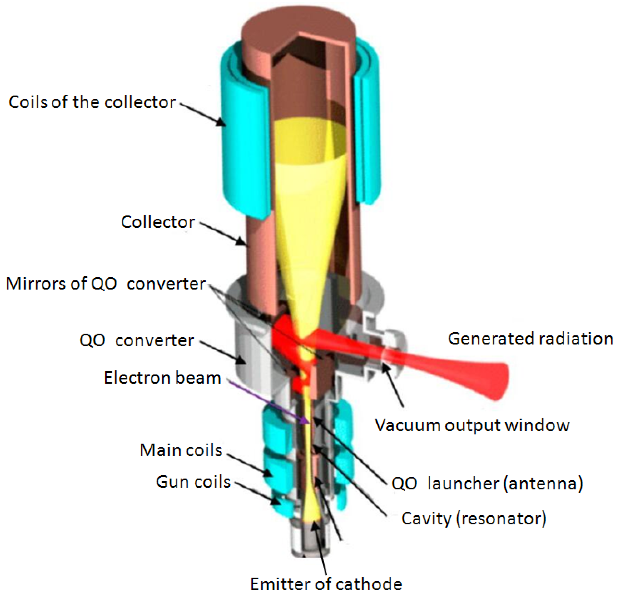
The structure and main parts of a gyrotron are shown schematically in Figure 1. The tube contains an electron-optical system (EOS) in which the initial formation of the electron beam is performed by a magnetron injection gun. It is then compressed in an adiabatically increasing magnetic field, and the energy of the orbiting electrons associated with their rotational motion increases at the expense of their axial momentum. The interaction between beam electrons and an electromagnetic wave takes place in the cavity resonator, where the magnetic field intensity reaches its maximum. The generated radiation is transformed into a well-collimated (Gaussian-like) wave beam by a quasi-optical (QO) mode converter comprising a launcher (of the Vlasov or Denisov type) and a system of mirrors. The output wave beam is coupled to the outside world through a vacuum window. The energy of the spent electron beam is dissipated in a water-cooled collector, which is equipped with magnetic coils used to evenly distribute the deposited energy and reduce the thermal load. In some of the most advanced designs (e.g., in gyrotrons for fusion), various sophisticated depressed collectors are used to recover some of the electron beam energy and increase overall efficiency. The example in Figure 1 with an internal mode converter and radial output of the generated radiation is typical for powerful gyrotrons for fusion. For other applications, sometimes more simple designs (e.g., without an internal mode converter and with an axial output of the wave) are used.

In this paper, we provide a comprehensive and systematic overview of some selected well-known fundamental analytical relations of gyrotron theory, which are usually treated separately and without sufficient details in otherwise excellent monographs on gyrotron physics (see, e.g., [15,16,17,18,19,20,21,22]). The focus here is on the important constants of electron motion (invariants) that are insightful for understanding the underlying mechanisms of beam–wave interaction in gyro-devices. We believe that a systematic and consistent presentation of these fundamentals of gyrotron theory in one place (and in the proper order) would be helpful to a wide readership, not limited to experts in the development and application of gyrotrons.

The paper is organized as follows: In Section 2, we consider the dispersion of electromagnetic waves in waveguides, transverse waves in electron beams, Brillouin dispersion diagrams, and cyclotron resonance conditions in beam–wave synchronization. Special attention is given to the derivation of the autoresonance integrals in the context of the CARM interaction. Section 3 is devoted to the analysis of the invariants of the equations describing the formation of helical electron beams in the electron-optical system (EOS) of gyrotrons, both conventional and large-orbit gyrotron (LOG). Finally, in Section 4, we draw a conclusion.

2. Electron Cyclotron Resonance, Cyclotron Autoresonance, and Brillouin Diagrams

2.1. Dispersion Equation of a Hollow Smooth-Wall Metallic Waveguide

The dispersion equation of a waveguide, which relates the longitudinal (axial) wavenumber $k_z$ (along the propagation axis z) to the frequency $\omega$ of the mode with a cut-off frequency ${\omega }_c$, is as follows:

$$\omega =\sqrt{{\omega }_c^2+c^2{k}_z^2},$$

(1)

where c is the speed of light in vacuum. This relation is plotted in Figure 2 in normalized coordinates $\frac{\omega }{{\omega }_c}$ and $\frac{k_z}{k_{\perp }}$, where $k_{\perp }=\frac{{\omega }_c}{c}$ is the transverse wavenumber. The cut-off frequency of a transverse (TE_mn or TM_mn mode) in a waveguide of radius R is ${\omega }_c=c\frac{{\chi }_{m,n}}{R}$, where ${\chi }_{m,n}$ is the eigenvalue of the mode (n-th root of the equation $\frac{d{J}_m\left(x\right)}{\mathrm{dx}}=0$ for the derivative of the Bessel function of first kind and order m in the case of a TE_mn mode, and of the equation $J_m\left(x\right)=0$ for a TM_mn mode, respectively). At an arbitrary point ($k_{\mathrm{z}0}$, ${\omega }_0$) of the dispersion curve (see Figure 2), the phase and group velocity of the wave are defined as follows:

$$v_{\mathrm{ph}}=\frac{{\omega }_0}{k_{z0}}\mathrm{and}{v}_{\mathrm{gr}}=\frac{d\omega }{d{k}_z}(k_{z0},{\omega }_0),$$

(2)

respectively, and are connected by the relation $v_{\mathrm{ph}}{v}_{\mathrm{gr}}=c^2$. Since the total wavenumber k is as follows:

$$k^2=\frac{{\omega }^2}{c^2}={k_{\perp }}^2+{k_z}^2,$$

(3)

the phase velocity normalized to the speed of light can be written in the following form:

$${\beta }_{\mathrm{ph}}=\frac{v_{\mathrm{ph}}}{c}=\sqrt{1+\frac{k_{\perp }^2}{k_z^2}}.$$

(4)

2.2. Transverse Waves in Electron Beams

In gyro-devices, helical electron beams are used in which the electrons gyrate in a strong magnetic field B with a relativistic cyclotron frequency ${\mathrm{\Omega }}_C$ given by the following:

$${\mathrm{\Omega }}_C=\frac{\mathrm{eB}}{\gamma m_0},$$

(5)

where e and $m_0$ are the charge and rest mass of an electron. Here, $\gamma$ is the relativistic Lorentz factor $\gamma ={(1-\frac{v^2}{c^2})}^{-1/2}={(1-\frac{v_z^2+v_{\perp }^2}{c^2})}^{-1/2}$, and $v_z$ and $v_{\perp }$ are the axial and transverse components of the total velocity v of the electron, respectively.

An electron beam of gyrating electrons drifting in the presence of an axial magnetic field supports two space-charge waves and two transverse cyclotron waves propagating along the beam axis [23,24,25]. Here, we consider only the latter since the former are not related to gyro-devices. The dispersion characteristics of the cyclotron waves (see Figure 3) are defined by the following:

$$\omega =\mp {\mathrm{\Omega }}_C+v_z{k}_z.$$

(6)

Here, the minus and plus signs correspond to SCWs (slow cyclotron waves) and FCWs (fast cyclotron waves), respectively. Their phase velocities depend on the axial velocity of beam electrons and on the angular cyclotron frequency and are given by the following:

$$v_{\mathrm{ph}}=\frac{v_z}{1\pm \frac{{\mathrm{\Omega }}_{\mathrm{C}}}{\omega }},$$

(7)

as shown in Figure 4. Therefore, the phase velocity of FCW can be greater than the axial velocity of the electron beam and, in the case of cyclotron resonance ($\omega ={\mathrm{\Omega }}_c$), can even become infinite. Moreover, depending on the direction (sign) of the phase velocity, FCW can be either forward or backward propagating. In contrast, the phase velocity of SCW is always smaller than the axial velocity of the beam electrons and positive, which means that it propagates in the forward direction.

The frequency $\omega$ defined by the dispersion Equation (6) for FCW can also be considered as a Doppler-shifted cyclotron frequency of the gyrating beam electrons or one of its harmonics. In order to investigate the most general cases, from now on, in the derivations that follow, we will use ${\mathrm{\Omega }}_{\mathrm{CH}}=s{\mathrm{\Omega }}_C(s=1,2,3,\dots )$, i.e., the harmonics of ${\mathrm{\Omega }}_c$ rather than the fundamental cyclotron frequency ${\mathrm{\Omega }}_C$. Before we proceed to that, however, it is important to mention that, here, we are considering an operation with the normal Doppler effect for which the frequency $\omega$ is larger than the Doppler term $v_z{k}_z$ and the resonance condition (6) is satisfied for positive harmonic numbers. Contrary to this, in cyclotron resonance devices based on the anomalous Doppler effect [26], $v_z{k}_z>\omega$ and the resonance condition occurs for negative harmonic numbers. Such a situation takes place if the phase velocity of the wave is smaller than the axial velocity of the electrons, i.e., in devices with slow-wave structures, which are beyond the scope of this paper.

For the subsequent considerations, it would be instructive to recall that, at the beam–wave synchronism of the electromagnetic field with time dependence ∼$e^{i\omega t}$, the phase of an electron with respect to the operating mode is as follows:

$$\theta =\omega t-k_{z}z-s\phi =\mathrm{const},$$

(8)

where $\phi$ is the angular coordinate of the electron. The differentiation of this equation with respect to time gives the following:

$$\omega -k_z{v}_z-s\dot{\phi }=0,$$

(9)

which, taking into account that $\dot{\phi }={\mathrm{\Omega }}_c$, coincides exactly with the electron cyclotron resonance condition (6) written there for $s=1$.

2.3. Beam–Wave Synchronism and Brillouin Diagrams

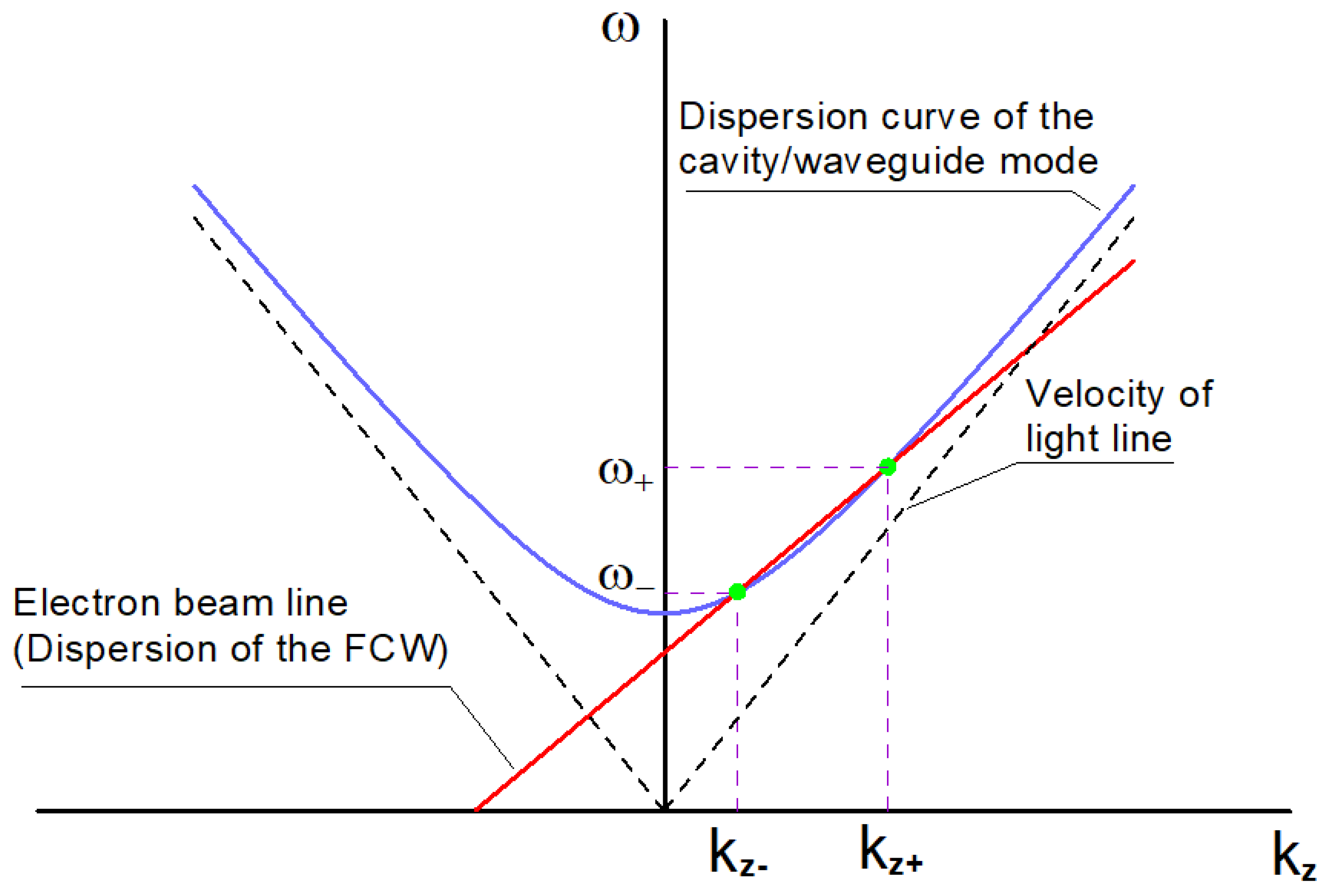
In fast-wave gyro-devices, a helical electron beam interacts with an electromagnetic wave excited in an electrodynamical system, which is a cavity resonator in the case of gyrotrons and gyro-klystrons or a waveguide structure as is in the case of gyro-TWT or gyro-BWO. The cyclotron resonance takes place when the waveguide mode is properly synchronized with FCW. The possible operating points, where such synchronism exists, correspond to the intersections of the beam line (dispersion equation of FCW):

$$\omega ={\mathrm{\Omega }}_{\mathrm{CH}}+v_z{k}_z$$

(10)

and the dispersion curve of the waveguide mode:

$${\omega }^2={\omega }_c^2+c^2{k}_z^2.$$

(11)

Their coordinates on the dispersion (Brillouin) diagram (see Figure 5) are given by the following:

$$k_{z_{+,-}}=\frac{{\mathrm{\Omega }}_{\mathrm{CH}}{\gamma }_z^2}{c}\left({\beta }_z\pm \sqrt{1-\frac{{\omega }_c^2}{{\gamma }_z^2{\mathrm{\Omega }}_{\mathrm{CH}}^2}}\right),$$

(12)

$${\omega }_{+,-}={\mathrm{\Omega }}_{\mathrm{CH}}{\gamma }_z^2\left(1\pm {\beta }_z\sqrt{1-\frac{{\omega }_c^2}{{\gamma }_z^2{\mathrm{\Omega }}_{\mathrm{CH}}^2}}\right).$$

(13)

Here, ${\beta }_z=v_z/c$ is the axial velocity of the beam electrons $v_z$, normalized to the speed of light in vacuum $c,$ and ${\gamma }_z=\frac{1}{\sqrt{1-{\beta }_z^2}}$.

An important parameter in these equations, which is sometimes called “waveguide parameter” is as follows [27]:

$$\mathrm{\Psi }=\frac{{\omega }_c^2}{{\gamma }_z^2{\mathrm{\Omega }}_{\mathrm{CH}}^2}.$$

(14)

Obviously, the case $\mathrm{\Psi }>1/{\gamma }_z^2$ (and thus ${\omega }_c>{\mathrm{\Omega }}_{\mathrm{CH}}$) corresponds to a forward operation which we consider first. When $\frac{1}{{\gamma }_z^2}<\mathrm{\Psi }<1$, there are two intersection points, as illustrated in Figure 5. The CARM interaction takes place at the upshifted frequency ${\omega }_{+}$, while the intersection at the lower frequency ${\omega }_{-}$ corresponds to a Gyro-TWT or gyrotron operation. In the latter case, the term of the Doppler shift is small, and therefore, the gyrotrons operate at frequencies close to the cyclotron frequency or its harmonics ($\omega \approx {\mathrm{\Omega }}_{\mathrm{CH}}=s{\mathrm{\Omega }}_C$).

A special case is the so-called grazing condition (coalescence between the field and the beam), shown in Figure 6. It is realized when $\mathrm{\Psi }=1$, i.e., when the following holds:

$${\omega }_c={\gamma }_z{\mathrm{\Omega }}_{\mathrm{CH}}.$$

(15)

In this particular case, the coordinates of the intersection point are as follows:

$$k_z=\frac{{\mathrm{\Omega }}_{\mathrm{CH}}{\gamma }_z^2{\beta }_z}{c}\mathrm{and}\omega ={\mathrm{\Omega }}_{\mathrm{CH}}{\gamma }_z^2.$$

(16)

Note that, at the grazing intersection (which is also called group synchronism) of the dispersion relation of the cyclotron resonance mode and the transverse waveguide/cavity mode, the velocity of the electrons is also equal to the group velocity, i.e., $v_z=v_{gr}=\frac{c^2}{v_{\mathrm{ph}}}$.

Figure 7 shows how the normalized frequencies at the lower and upper intersections of the Brillouin diagram change with increasing the magnetic field intensity (and thus ${\mathrm{\Omega }}_{\mathrm{CH}}$).

At $\mathrm{\Psi }=\frac{1}{{\gamma }_z^2}$, $\omega ={\omega }_c={\mathrm{\Omega }}_{\mathrm{CH}}$ and the beam line passes through the vertex of the hyperbola of the waveguide mode. If $\mathrm{\Psi }<\frac{1}{{\gamma }_z^2}$, however (when ${\mathrm{\Omega }}_{\mathrm{CH}}>{\omega }_c$), $k_{z_{-}}<0$ and the electron beam interacts with a backward propagating wave (see Figure 8) for which both the group and phase velocity are negative.

For a given mode, the operating point can be controlled by varying separately or simultaneously two parameters of the electron beam, namely, the axial velocity $v_z$ and the harmonic cyclotron frequency ${\mathrm{\Omega }}_{\mathrm{CH}}$. Varying $v_z$, the slope of the beam line is changed, while by varying ${\mathrm{\Omega }}_{\mathrm{CH}}$, the beam line is translated parallel to itself.

It is instructive also to show that the equations of beam lines passing through an arbitrary intersection point with coordinates ($k_{\mathrm{z}0}$, ${\omega }_0)$ can be written in the following two equivalent forms:

$$\omega ={\mathrm{\Omega }}_{CH}+\frac{{\omega }_0-{\mathrm{\Omega }}_{CH}}{k_{z0}}{k}_z$$

(17)

or

$$\omega ={\omega }_0+{c{\beta }_z{(k}_z-k}_{z0}).$$

(18)

Here, $\frac{{\mathrm{\Omega }}_{\mathrm{CH}}}{\gamma }$ and $c{\beta }_z$ are parameters different for each beam line of the bundle. From the resonance condition at the intersection point, we obtain the following:

$$\frac{{\mathrm{\Omega }}_{\mathrm{CH}}}{{\omega }_0}=1-{\beta }_z/{\beta }_{\mathrm{ph}}.$$

(19)

For the following analysis (in Section 2.4), however, it is convenient to express (using Equation (10)) the frequency at the resonance as follows:

$$\omega =\frac{s{\mathrm{\Omega }}_{CS}}{\gamma (1-\frac{{\beta }_z}{{\beta }_{\mathrm{ph}}})}.$$

(20)

Here, we use the nonrelativistic cyclotron frequency ${\mathrm{\Omega }}_{CS}=eB/m_0$ to show explicitly the dependence of the operating frequency on the harmonic number s and the relativistic factor $\gamma$.

In the dispersion diagrams above, the waveguide modes are represented by continuous curves, which is legitimate for the continuous spectrum of the hollow metallic waveguide. However, in the cavity resonators, the spectrum is discrete, and therefore, the corresponding resonances can be represented by points lying on the hyperbola and having a discrete set of the axial wavenumbers given by the following:

$$k_z=\frac{q\pi }{L_{\mathrm{ef}}},$$

(21)

where the axial mode index q is an integer number and $L_{\mathrm{ef}}$ is the effective length of the resonator. This means that resonances are possible for a sequence of high-order (q > 1) forward or backward axial modes (HOAM), as illustrated in Figure 9. Generally, the axial mode index q corresponds to the number of the field variations along the cavity axis. The axial field profile is described by the Helmholtz equation, which is supplemented by certain boundary conditions. The analysis of the solutions of this equation leads to a more detailed picture of the resonances with finite bandwidths and is discussed in [28]. According to this approach, the resonances should be represented by zones (bands) rather than points. This concept is illustrated in Figure 9. It has been shown (and demonstrated experimentally [29,30,31,32,33,34,35]) that, by exciting a sequence of successive HOAM, continuous frequency tuning can be performed simply by changing the magnetic field intensity (and hence ${\mathrm{\Omega }}_{\mathrm{CH}}$).

One further remark is in order at this point. The FCW line in the dispersion diagrams represents an idealized monoenergetic electron beam without velocity scattering (distribution). Therefore, such line should be considered as the result of averaging, or alternatively, one should consider different lines for the different fractions of beam electrons.

For simplicity, in the above illustrative examples, we have considered only the possible operating points (resonances) of a single cavity mode. In reality, however, there is a dense spectrum of nonequidistant modes in the gyrotron resonant cavity, and therefore, many intersections of the beam lines (corresponding to different harmonics) and dispersion curves of various modes are possible. This is illustrated in Figure 10. The density of the mode spectrum (which increases with frequency) and the finite bandwidth of the resonances are responsible for mode competition—a severe problem in selecting a suitable mode and operating the gyrotron in a single mode regime (i.e., without exciting spurious parasitic modes). This subject is discussed in detail in the recently published comprehensive review paper [36].

At resonance, the electrons of the beam interact efficiently with the operating mode. As a result of this interaction, depending on their phase with respect to the wave, some of them lose energy and thus transfer part of their rotational kinetic energy to the wave, while the rest gain energy at the expense of the wave energy. Due to the dependence of the cyclotron frequency on energy (see Equation (5)), the former (with decreased $\gamma$) rotate faster in contrast with the latter (with increased $\gamma$), which rotate slower. This leads to azimuthal bunching of the electrons. With proper synchronization, when the operating frequency exceeds the cyclotron frequency, the formed bunch slips in phase toward the decelerating phase of the cavity mode, where the electrons lose energy due to bremsstrahlung and transfer it up to the wave. The mechanism described is known as electron cyclotron maser instability, and accordingly, the gyrotrons are also called electron cyclotron masers (CRMs). Recall that “maser” stands for microwave amplification by stimulated emission of radiation. It should be mentioned, however, that this term is more or less an archaism nowadays, since the gyrotrons have already advanced to the THz frequency band. An adequate description of the physics of the underlying mechanism from a quantum mechanical point of view and in the framework of the relativistic electrodynamics can be found in numerous publications and monographs (see, e.g., [16,17,18,19,20]).

2.4. Cyclotron Autoresonance and CARM

In this subsection, we consider a special case of synchronization between the electron beam and the electromagnetic wave known as electron cyclotron autoresonance (CAR) (or self-sustained gyro-resonance). This phenomenon was independently discovered by V. Ya. Davydovsky [37] and A. A. Kolomensky with A. N. Lebedev [38]. Soon thereafter, studies on this subject attracted considerable interest, and new concepts for devices generating electromagnetic radiation [39,40,41,42,43,44] and particle accelerators [45,46,47,48,49] based on such resonance were formulated and demonstrated. These studies are well presented in comprehensive review articles [50,51].

From the analysis of the cyclotron resonance condition (Equation (10)), it appears that, during the interaction between the beam electrons and the wave, both the cyclotron frequency and the Doppler shit term change, but in opposite directions. As pointed out by the discoverers of CAR (and then confirmed in corresponding derivations and experiments by many other authors (in addition to [39,40,41,42,43,44], see also the following list of selected references [52,53,54,55,56,57,58,59]), at large axial velocities (and hence large Doppler up-shift), the operating point asymptotically approaches the intersection point, where the phase velocity is close to the speed of light and the changes in the two terms completely compensate (cancel) each other. Therefore, the beam and the wave remain synchronized, and the resonance is self-sustaining, as illustrated in Figure 11. In other words, at such a specific operating point, if the cyclotron resonance condition is initially fulfilled, it will be maintained despite the changes in energy during the beam–wave interaction.

The scientists who discovered CAR envisaged the application of this remarkable phenomenon to particle acceleration—the so-called CARA (cyclotron autoresonance acceleration), which has been studied by many researchers (see, for example, [45,46,47,48,49]). This topic, however, is outside the scope of the present work, and we discuss here only the underlying importance of CAR for CARM devices.

Cyclotron autoresonance is possible due to the existence of a fundamental invariant—a constant of electron motion, which we describe below. Its derivation is very straightforward, concise, and insightful. That is why we reproduce it briefly here following [60].

First, we consider the axial component of the relativistic equation of electron motion in a TE wave:

$$\frac{d}{dt}\left(m_0\gamma v_z\right)=-e{({\overrightarrow{v}}_{\perp }\times {\overrightarrow{B}}_{\perp })}_z$$

(22)

and the equation that describes the change in its energy:

$$\frac{d\gamma }{dt}=-\frac{e}{m_0{c}^2}{\overrightarrow{v}}_{\perp }·{\overrightarrow{E}}_{\perp }$$

(23)

where ${\overrightarrow{v}}_{\perp }$ is the transverse velocity of an electron and ${\overrightarrow{E}}_{\perp },{\overrightarrow{B}}_{\perp }$ are the transverse electric and magnetic fields of the wave, respectively. The magnitudes of these fields are related by the wave impedance Z through the following equation (written in vector notations):

$$Z{\overrightarrow{H}}_{\perp }={\overrightarrow{z}}_{\perp }\times {\overrightarrow{E}}_{\perp },$$

(24)

where the magnetic field strength $H={\mu }_{0}B$ and ${\mu }_0$ is the permeability of free space. Using a polar coordinate system $(r,\varphi ,z)$ and complex notations:

$$E_{\perp }=E_r+i{E}_{\varphi };H_{\perp }=H_r+i{H}_{\varphi },$$

(25)

the relations between the azimuthal and radial components of the electric and magnetic fields (marked by indices $\varphi$ and r, respectively) can be written in the following scalar form:

$$Z=\frac{E_r}{H_{\varphi }}=-\frac{E_{\varphi }}{H_r}.$$

(26)

The impedances of the TE and TM modes are given by the following relations:

$$Z^{TE}=Z_0\frac{k}{k_z}=Z_0\frac{v_{\mathrm{ph}}}{c}={\mu }_0{v}_{\mathrm{ph}},$$

(27)

$$Z^{TM}=Z_0\frac{k_z}{k}=Z_0\frac{c}{v_{\mathrm{ph}}}=\frac{{\mu }_0{c}^2}{v_{\mathrm{ph}}},$$

(28)

where $Z_0=\sqrt{{\mu }_0/{ϵ}_0}$ is the characteristic impedance of the free space, ${\epsilon }_0$ is permittivity of vacuum, and the following:

$$v_{\mathrm{ph}}=\frac{c}{\sqrt{1-\frac{k_{\perp }^2}{k^2}}},$$

(29)

is the phase velocity of the waveguide mode (compare with the phase velocity of FCW given in Equation (7)).

For the case of TE modes, using Equations (24) and (27), we express the right-hand side of (22) in terms of the transverse electric field and rewrite this equation in the following form:

$$\frac{d}{dt}\left(m_0\gamma v_z\right)=-\frac{e}{v_{\mathrm{ph}}}e({\overrightarrow{v}}_{\perp }·{\overrightarrow{E}}_{\perp }).$$

(30)

Canceling the term ${\overrightarrow{v}}_{\perp }·{\overrightarrow{E}}_{\perp }$ in (23) and (30), we obtain immediately the following important integral (an exact constant of motion):

$$\gamma \left(1-{\beta }_{\mathrm{ph}}{\beta }_z\right)={\gamma }_0\left(1-{\beta }_{\mathrm{ph}}{\beta }_{z0}\right)=I^{\mathrm{TE}}=\mathrm{const},$$

(31)

where ${\gamma }_0$ and ${\beta }_{z0}$ are the initial values of $\gamma$ and ${\beta }_z$.

If $v_{ph}\gg 1$, as is the case with gyrotrons operating at frequencies near the cut-off frequency of the resonant cavity (when $k\approx k_{\perp }$), this invariant reduces approximately to the conservation of the axial momentum, i.e., $p_z=m_0\gamma v_z=\mathrm{const}$.

The above constant of motion applies both to TE modes in waveguides or cavity resonators and to TEM waves in free space. In the latter case, the analysis is analogous but takes into account that the phase velocity of TEM waves is equal to the speed of light in vacuum.

Next, we consider electron motion in the field of TM modes. In addition to the difference in wave impedance, TE and TE modes also differ in that the TM waves have an axial component of the electric field $E_z$, and instead of Equations (22) and (23), we have the following:

$$\frac{d}{dt}\left(m_0\gamma v_z\right)=-e{({\overrightarrow{v}}_{\perp }\times {\overrightarrow{B}}_{\perp })}_z-e{E}_z$$

(32)

and

$$\frac{d\gamma }{dt}=-\frac{e}{m_0{c}^2}({\overrightarrow{v}}_{\perp }·{\overrightarrow{E}}_{\perp }+{\overrightarrow{v}}_z·{\overrightarrow{E}}_z).$$

(33)

Physically, this means that the axial momentum changes not only as a result of the recoil effect, but also due to the direct interaction with the axial component of the electric field of the TM wave.

Following the same approach as before, we express the transverse magnetic field of the TM mode through the corresponding transverse electric field using (24) and (28). In such a way, we rewrite (32) in the following form:

$$\frac{d}{dt}\left(m_0\gamma v_z\right)=-\frac{e{v}_{ph}}{c^2}{\overrightarrow{v}}_{\perp }·{\overrightarrow{E}}_{\perp }-e{E}_z.$$

(34)

From the comparison of (33) and (34), we obtain the following:

$$\frac{d}{dt}[\gamma (1-\frac{v_z}{v_{\mathrm{ph}}})]=\frac{e}{m_0{c}^2}(\frac{c^2}{v_{\mathrm{ph}}}-v_z)E_z.$$

(35)

It is easy to see that the right-hand side of this equation is small and even disappears altogether at grazing incidence (group synchronism). Moreover, the axial electric field (as seen by an electron propagating with an axial velocity significantly different from the phase velocity of the wave) is a rapidly changing time-harmonic function, and as shown in [60], its contribution averaged over the period is zero. Therefore, from (34), we obtain the following approximate constant of motion (invariant):

$$\gamma \left(1-\frac{{\beta }_z}{{\beta }_{\mathrm{ph}}}\right)={\gamma }_0\left(1-\frac{{\beta }_{z0}}{{\beta }_{\mathrm{ph}}}\right)=I^{\mathrm{TM}}=\mathrm{const}.$$

(36)

The invariants derived above (also known as autoresonance integrals) can be represented in the following unified (general) form, which is valid to both types of modes:

$$\gamma \left(1-\frac{Z}{Z_0}{\beta }_z\right)=\mathrm{const},$$

(37)

where ${Z=Z}^{\mathrm{TE}}$ or ${Z=Z}^{\mathrm{TM}}$, but bearing in mind that, in the first case, it is an exact constant, while in the second case, it is an approximate constant.

Returning to the resonance condition (20), one can see that the denominator coincides with the constant of motion for TE modes only if ${\beta }_{\mathrm{ph}}=1$ (when $I^{\mathrm{TE}}=\gamma \left(1-{\beta }_z\right)=\mathrm{const}$) and hence $\omega =\frac{s{\mathrm{\Omega }}_C}{\gamma (1-{\beta }_z)}$. In contrast, for the TM modes, the synchronism is observed for any phase velocity and $\omega =\frac{s{\mathrm{\Omega }}_C}{\gamma (1-\frac{{\beta }_z}{{\beta }_{\mathrm{ph}}})}$. In general, for CARM interaction (when ${\beta }_{\mathrm{ph}}\to 1$), the constants of motion for the TE and TM modes coincide, and we have $I^{\mathrm{TE}}=\gamma \left(1-{\beta }_z\right)=I^{\mathrm{TM}}$.

The above considerations could be “translated” in the language of quantum physics. For a single electron emitting a photon, the changes in its energy and axial momentum are $\Delta E=\hslash \omega$ and $\Delta p_z=\hslash k_z$, respectively (ℏ being Planck’s constant), and therefore, $\frac{\Delta E}{\Delta p_z}=\frac{\omega }{k_z}=c{\beta }_{\mathrm{ph}}$. Thus, when an electron is decelerated in a forward wave ($k_z>0$), its axial momentum decreases. On the contrary, when it is decelerated in a backward propagating wave, $p_z$ increases. Near the cut-off frequency, where ${\beta }_{ph}\to 0$, the momentum does not change. In the case of ${\beta }_{ph}=1$ (as follows from (31) and (36)), momentum and energy change in such a way that $\gamma (1-{\beta }_z)=\mathrm{const}.$

Besides the importance of these invariants for the existence of CAR, they also provide a deeper insight on the relation between the physical parameters affecting the beam–wave interaction and allow some important properties of electron motion to be deduced. For example, using the constants of motion, it is possible and instructive to express the axial and the transverse velocities of the electron as functions of the energy only (or $\gamma$). For the TE modes, the relations are as follows:

$${\beta }_z=\frac{\gamma -I^{\mathrm{TE}}}{\gamma {\beta }_{\mathrm{ph}}};{\beta }_{\perp }=\frac{1}{\gamma }{\left[{\gamma }^2-1-{\left(\frac{\gamma -I^{\mathrm{TE}}}{{\beta }_{\mathrm{ph}}}\right)}^2\right]}^{1/2}.$$

(38)

In addition, analogously, for TM modes, we have the following:

$${\beta }_z=\frac{{\beta }_{\mathrm{ph}}}{\gamma }(\gamma -I^{\mathrm{TM}});{\beta }_{\perp }=\frac{1}{\gamma }{\left[{\gamma }^2-1-{\beta }_{\mathrm{ph}}^2{\left({\gamma }^2-I^{\mathrm{TM}}\right)}^2\right]}^{1/2}.$$

(39)

Another observation, which gives physical insight, is that these constants of motion are satisfied even for a completely spent electron beam, i.e., when $\gamma =1$ and ${\beta }_z=0$ provided that the initial parameters satisfy the following conditions:

$${\beta }_{z0}=\frac{1}{{\beta }_{ph}}(1-\frac{1}{{\gamma }_0}),$$

(40)

for TE modes, and

$${\beta }_{z0}={\beta }_{\mathrm{ph}}(1-\frac{1}{{\gamma }_0}),$$

(41)

for TM modes. It should be mentioned, however, that the latter conditions are necessary but not sufficient in order to extract the whole energy of the electron beam.

During the interaction, the energy of an electron:

$$W=m_0{c}^2\gamma =m_0{c}^2\sqrt{1+\frac{p_{\perp }^2+p_z^2}{m_0^2{c}^2}},$$

(42)

changes according to the following equation:

$$\frac{\mathrm{dW}}{\mathrm{dt}}=v_{\perp }\frac{d{p}_{\perp }}{\mathrm{dt}}+v_z\frac{d{p}_z}{\mathrm{dt}},$$

(43)

where (as above) $p_{\perp }$, $p_z$, $v_{\perp }$, and $v_z$ are the transverse and axial moments and velocities, respectively. From this equation and the autoresonance integral for the TE modes, it follows that the following holds:

$$v_{\perp }\frac{d{p}_{\perp }}{\mathrm{dt}}=(1-\frac{{\beta }_z}{{\beta }_{\mathrm{ph}}})\frac{\mathrm{dW}}{\mathrm{dt}},v_z\frac{d{p}_z}{\mathrm{dt}}=\frac{{\beta }_z}{{\beta }_{\mathrm{ph}}}\frac{\mathrm{dW}}{\mathrm{dt}}.$$

(44)

In the case of gyrotron operation, ${1/\beta }_{\mathrm{ph}}\ll 1$, and therefore, the second term can be neglected. However, in the case of CARM operation, energy extraction from the axial momentum also takes place. In general, the ratio between the second and the first term in Equation (43) is as follows:

$$\frac{v_z\frac{d{p}_z}{\mathrm{dz}}}{v_{\perp }\frac{d{p}_{\perp }}{\mathrm{dz}}}=\frac{{\beta }_z\gamma }{{\beta }_{\mathrm{ph}}}{\mathrm{\Gamma }}^{\mathrm{TE}},$$

(45)

where the factor ${\mathrm{\Gamma }}^{\mathrm{TE}}=\frac{\omega }{{\mathrm{\Omega }}_{\mathrm{CH}}}={\left[\gamma \left(1-\frac{{\beta }_z}{{\beta }_{\mathrm{ph}}}\right)\right]}^{-1}$ gives the ratio between the upshifted resonant frequency and the nonrelativistic cyclotron frequency.

Analogously, for TM modes, we have the following:

$$v_{\perp }\frac{d{p}_{\perp }}{\mathrm{dt}}=(1-\frac{{\beta }_z}{{\beta }_{\mathrm{gr}}})\frac{\mathrm{dW}}{\mathrm{dt}},v_z\frac{d{p}_z}{\mathrm{dt}}=\frac{{\beta }_z}{{\beta }_{\mathrm{gr}}}\frac{\mathrm{dW}}{\mathrm{dt}},$$

(46)

and

$$\frac{v_z\frac{d{p}_z}{\mathrm{dz}}}{v_{\perp }\frac{d{p}_{\perp }}{\mathrm{dz}}}=\frac{{\beta }_z\gamma }{{\beta }_{\mathrm{gr}}}{\mathrm{\Gamma }}^{\mathrm{TM}},$$

(47)

where ${\mathrm{\Gamma }}^{\mathrm{TM}}={\left[\gamma \left(1-\frac{{\beta }_z}{{\beta }_{\mathrm{gr}}}\right)\right]}^{-1}$.

Note that these relations are similar to (44), but everywhere the phase velocity is replaced by the group velocity of the wave in order to preserve their structure. Of course, they can also be written using the phase velocity and the relation ${\beta }_{\mathrm{ph}}{\beta }_{\mathrm{gr}}=1$.

In the case of TE modes, the limiting single-particle efficiency of the beam–wave interaction is given in [40] and reads as follows:

$${\eta }_{\mathrm{sp}}=\frac{{\beta }_{\perp 0}^2}{2(1-{\beta }_{z0/{\beta }_{\mathrm{ph}}})\left(1-{\gamma }_0^{-1}\right)}.$$

(48)

Using the constant of motion ${\mathrm{\Gamma }}^{\mathrm{TE}}$, it can be expressed in the following more compact form:

$${\eta }_{\mathrm{sp}}=\frac{{\beta }_{\perp 0}^2{\gamma }_0^2{\mathrm{\Gamma }}_0^{\mathrm{TE}}}{2({\gamma }_0-1)}.$$

(49)

Another important parameter is the so-called electron recoil parameter [16,40,54]:

$$b=\frac{{\gamma }_0{\beta }_{\perp 0}^2}{2{\beta }_{z0}{\beta }_{\mathrm{ph}}(1-\frac{{\beta }_{z0}}{{\beta }_{\mathrm{ph}}})},$$

(50)

which characterizes how the axial momentum varies with beam energy. The larger b is, the faster the axial momentum decreases with the decrease in $\gamma$ [54]. For the gyrotron operation, $b\approx 0$, while for CARM, the typical values are in the range 0.2–0.5 or greater [40]. Plots of optimal normalized efficiency are given by Fliflet (see Figures 1 and 2 in [54]). The knowledge of the parameter b allows one to evaluate the single-particle efficiency from these plots without solving again the equations of motion.

3. Equations of Motion of Gyrating Electrons and Their Invariants (Integrals of Motion) Describing the Formation of Helical Electron Beams in the Electron-Optical System (EOS) of Gyrotrons

In the previous sections, we considered some of the basic relationships relevant to the resonance conditions and beam–wave interaction in gyro-devices. In this section, we discuss some important analytical expressions (including the constants of motion) that describe the formation of helical electron beams used in these tubes.

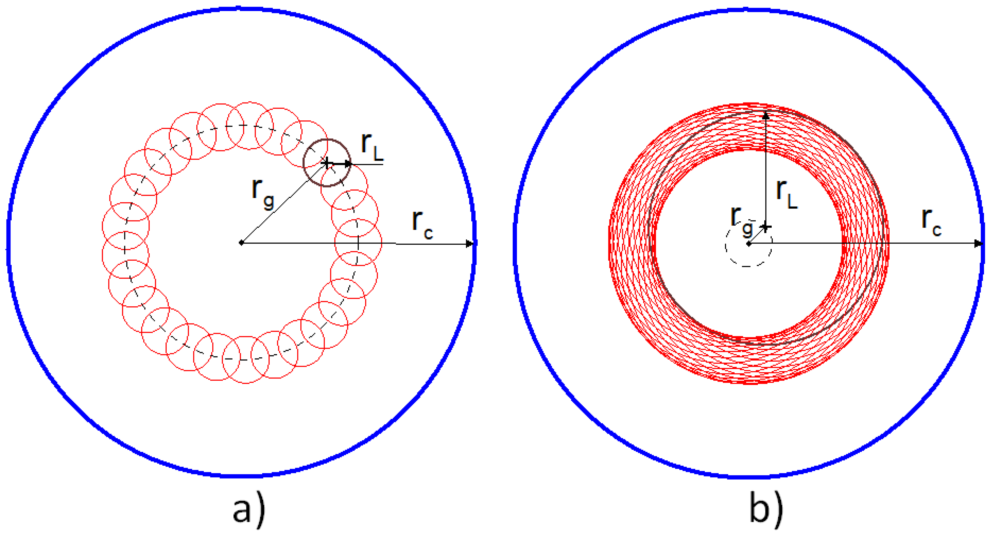
As mentioned above, the active medium in gyro-devices is an electron beam interacting with a fast wave (i.e., with a phase velocity greater than the speed of light in vacuum) in the electrodynamic system (resonant cavity or waveguide), where the beam is synchronized with the electromagnetic wave according to the cyclotron resonance conditions explained above. Usually, two types of beams are used (see Figure 12). The first, used in conventional gyrotrons, is a polyhelical hollow (tubular) electron beam in which the individual orbiting electrons follow helical trajectories whose guiding centers are at a certain distance (radius of the guiding center $r_g$) from the axis. The second type, used in the so-called large orbit gyrotron (LOG) (see, for instance, [61,62,63,64]), is usually referred to as an axis-encircling (or uniaxial) electron beam since the individual orbits encircle the axis and their radius is comparable to the radius of the resonator, in contrast with conventional devices where the electrons gyrate around their axes, following helices with a much smaller radius. The helical electron beam is formed in an electron-optical system (EOS) using a magnetron injection gun (MIG), in which the electrons are accelerated and their orbits twisted in crossed electric and magnetic fields. More sophisticated EOSs are used to generate uniaxial electron beams, which include a cusp electron gun or a kicker (special magnetic coils).

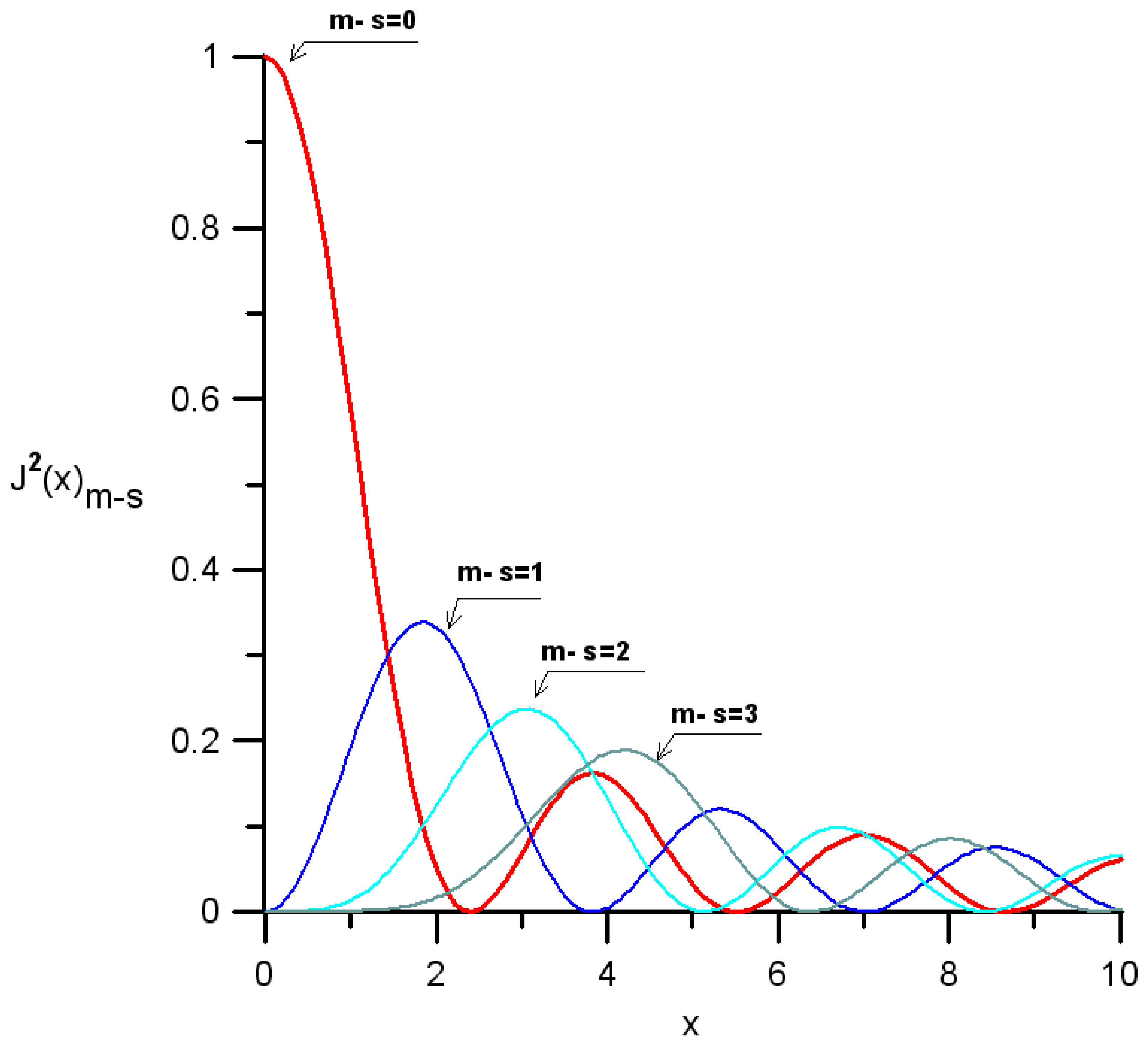
LOG operation is inherently high harmonic, since the uniaxial electron beam interacts only with ${\mathrm{TE}}_{mn}$ modes whose axial index m equals the harmonic number ($m=s$) and can be significantly greater than unity. For the same reason, LOG offers an increased mode selectivity. This follows from the analysis of the coupling coefficient G, which characterizes the strength of the beam–wave interaction as a function of the beam radius:

$$G=\frac{J_{m-s}^2\left({\chi }_{mn}\frac{R_b}{R_c}\right)}{\left({\chi }_{mn}^2-m^2\right)J_m^2\left({\chi }_{mn}\right)},$$

(51)

where $R_b$ and $R_c$ are the beam radius and the cavity radius, respectively. If $m-s\ne 0$, $G=0$ for $R_b=r_g=0$ (see Figure 13). Therefore, the electron beam in LOG couples effectively only with the corotating modes whose azimuthal indices are equal to the harmonic number.

In both cases, the electron beams (either polihelical or uniaxial) then propagate in an increasing magnetic field where the transverse velocity of the electrons gradually increases at the expense of their axial velocity. This process is habitually called “pumping” since the energy related to the transverse motion is being transferred to the electromagnetic field during the beam–wave interaction that takes place in the electrodynamical system of gyrotrons (here we do not consider CARM in which, as was shown, energy is extracted also from the axial momentum).

Before going into detail, we introduce some basic relationships and notations that will be used below. The gyrating electrons move in the transverse plane on circular orbits with a cyclotron angular velocity ${\mathrm{\Omega }}_C$ and drift in the axial direction on helical trajectories with a pitch $l=T_c{v}_z$, where $T_c=2\pi /{\mathrm{\Omega }}_C$ is the cyclotron period. The instantaneous radius of the circular orbit (also called Larmor radius) is $r_L=v_{\perp }/{\mathrm{\Omega }}_C$. As mentioned earlier, the relativistic dependence of ${\mathrm{\Omega }}_C$ on the energy ($\gamma$) of the electrons forming the beam leads to their nonisochronous motion and is responsible for one of the most essential mechanisms, namely, azimuthal bunching, which takes place at a cyclotron resonance as described above.

In a cylindrical coordinate system (r, $\phi$, z), the relativistic equation of motion of an electron under the action of an electric field $\overrightarrow{E}$ and a magnetic field $\overrightarrow{B}$ is as follows:

$$\frac{d}{\mathrm{dt}}\left(m\overrightarrow{v}\right)=-e\left[\overrightarrow{E}\left(\overrightarrow{r,}t\right)+\overrightarrow{v}\times \overrightarrow{B}\left(\overrightarrow{r,}t\right)\right].$$

(52)

Taking the vector product of both sides with $\overrightarrow{r}$ and considering only the axial projection (component), we readily obtain the following:

$$\frac{d}{\mathrm{dt}}\left(m{r}^2\dot{\phi }\right)=-er(E_{\phi }+\dot{z}{B}_r-\dot{r}{B}_z).$$

(53)

The forces acting on the electron are shown in Figure 14. In an axially symmetric EOS, the axial $B_z$ and the radial $B_r$ components of the static magnetic field $\overrightarrow{B}=\mathrm{curl}\left(\overrightarrow{A}\right)$ can be expressed through the azimuthal component $A_{\phi }$ of the vector potential $\overrightarrow{A}$ (since, for such symmetry, $A_r=A_z=0$ and $B_{\phi }=0$) as follows:

$$B_z=\frac{1}{r}\frac{\partial \left(r{A}_{\phi }\right)}{\partial r},B_r=-\frac{1}{r}\frac{\partial \left(r{A}_{\phi }\right)}{\partial z}.$$

(54)

Furthermore, by virtue of the assumed symmetry, the azimuthal component of the static electric field in the EOS is absent. However, the change of the magnetic flux $\mathrm{\Phi }=2\pi r{A}_{\phi }$ through a circle of radius r and centered on the axis gives rise to an azimuthal electric field component that can be obtained from Faraday’s law:

$$\oint E_{\phi }dl=-\frac{\partial \mathrm{\Phi }}{\partial t}$$

(55)

and reads as follows:

$$E_{\phi }=-\frac{1}{r}\frac{\partial \left(r{A}_{\phi }\right)}{\partial t}.$$

(56)

This being performed, Equation (52) yields the following:

$$\frac{d}{\mathrm{dt}}(\gamma m_0{r}^2\dot{\phi }-er{A}_{\phi })=\frac{d{p}_{\phi }}{\mathrm{dt}}=0,$$

(57)

and therefore, the canonical angular momentum $p_{\phi }$ is conserved, i.e.,

$$p_{\phi }=\gamma m_0{r}^2\dot{\phi }-er{A}_{\phi }=\mathrm{const}.$$

(58)

Even a more elegant, concise, and insightful derivation of the above invariant can be performed by simply analyzing the Hamiltonian equations of motion in a cylindrical coordinate system ($r,\phi ,z$):

$${\dot{p}}_r=-\frac{\partial H}{\partial r},{\dot{p}}_{\phi }=-\frac{\partial H}{\partial \phi },{\dot{p}}_z=-\frac{\partial H}{\partial z},$$

(59)

$$\dot{r}=\frac{\partial H}{\partial p_r},\dot{\phi }=\frac{\partial H}{\partial p_{\phi }},\dot{z}=\frac{\partial H}{\partial p_z},$$

(60)

where the Hamiltonian H for axially symmetric fields ($\frac{\partial }{\partial \phi }=0$) is as follows:

$$H=\frac{1}{2m_0\gamma }\left[p_r^2+\frac{1}{r^2}{\left(p_{\phi }+er{A}_{\varphi }(r,z)\right)}^2+p_z^2\right]-eU(r,z),$$

(61)

and U is the axially symmetrical electrostatic potential. By virtue of the fact that this Hamiltonian does not depend explicitly on $\phi$, we have the following:

$${\dot{p}}_{\phi }=-\frac{\partial H}{\partial \phi }=0\mathrm{and},\mathrm{therefore},p_{\phi }=\mathrm{const},$$

(62)

which proves that the canonical angular momentum is an invariant (constant of motion). At the same time, since the following holds:

$$\dot{\phi }=\frac{\partial H}{\partial p_{\phi }}=\frac{1}{m_0\gamma r^2}(p_{\phi }+er{A}_{\varphi }(r,z)),$$

(63)

it follows that $p_{\phi }=\gamma m_0{r}^2\dot{\phi }-er{A}_{\phi }$, which, combined with (61), exactly coincides with (57).

Another invariant is the Hamiltonian itself, which is equal to the total energy of an electron and is explicitly independent of time, i.e., $H=\mathrm{const}$ since $\frac{dH}{dt}=\frac{\partial H}{\partial t}=0$.

In a paraxial approximation, $A_{\phi }\approx \frac{1}{2}{B}_0\left(z\right)r$, and we have the following:

$$p_{\phi }=\gamma m_0{r}^2\dot{\phi }-\frac{1}{2}e{B}_0{r}^2=C=\mathrm{const}.$$

(64)

Then, considering the point P (see Figure 15) on the orbit for which ${r=r}_g+r_L$, $v_r=0$, and $v_{\phi }=v_{\perp }={\mathrm{\Omega }}_C{r}_L$(recall than ${v_{\perp }}^2={v_r}^2+{v_{\phi }}^2$), we find the following:

$$C=\frac{1}{2}e{B}_0\left({r_L}^2-{r_g}^2\right).$$

(65)

Applying (63) to the cathode with the radius $r_c$, where the magnetic field is $B_c$ and $\dot{\phi }=0$, we obtain $B_c{r_c}^2=B_0({r_g}^2-{r_L}^2)$.

In electron optics, neglecting the relativistic dependence of the mass of electrons, the above invariant is usually written in the following form:

$$m_0{r}^2\dot{\phi }-\frac{e\mathrm{\Phi }}{2\pi }=\mathrm{const},$$

(66)

and is known as Busch’s theorem. Specifying the initial values at time t = 0 as ${r=r}_0,$ $\phi ={\phi }_0,$ and $\mathrm{\Phi }={\mathrm{\Phi }}_0$, respectively, gives the following:

$$r^2\dot{\phi }-r_0^2{\dot{\phi }}_0=-\frac{e}{2\pi m_0}(\mathrm{\Phi }-{\mathrm{\Phi }}_0).$$

(67)

Therefore, Busch’s theorem states that the change in angular velocity (an thus in angular momentum) between two axial positions depends only on the change in the total magnetic flux but is independent of the electron trajectory between these cross sections.

The generalized formulation of Busch’s theorem derived in [65] has the following form:

$${\oint }_C\overrightarrow{\mathrm{v}.}d\overrightarrow{C}+\frac{e}{m_0}\mathrm{\Phi }=\mathrm{const}.$$

(68)

Here, the path integral of the stream of electrons with velocities $\overrightarrow{v}$ is taken along a closed contour C confining a fixed set of possible particle trajectories, and $\mathrm{\Phi }$ is the magnetic flux through the area enclosed by C. This generalization extends the theorem to many particles in an electron beam without axial symmetry.

It is important to underline that one should account for the directions of the magnetic fluxes. More specifically, if a reverse of the magnetic field is present between the cross sections where $\mathrm{\Phi }$ and ${\mathrm{\Phi }}_0$ are considered, then the following holds:

$$r^2\dot{\phi }-r_0^2{\dot{\phi }}_0=-\frac{e}{2\pi m_0}(\mathrm{\Phi }+\left|{\mathrm{\Phi }}_0\right|).$$

(69)

Therefore, in the latter case, the gyrating electrons acquire an additional “twisting”.

It is easy to show that the conservation of the canonical angular momentum in the presence of magnetic field reversal leads to the formation of an axis-encircling electron beam. Consider Equation (64) at two cross sections, namely, before and after the reversal (cusp), marked by indices 1 and 2:

$$\frac{1}{2}e{B}_1\left({r_{L1}}^2-{r_{g1}}^2\right)=-\frac{1}{2}e{B}_2\left({r_{L2}}^2-{r_{g2}}^2\right).$$

(70)

If before the cusp, $r_{g1}>r_{L1}$, then after the cusp, where the magnetic field changes its direction (from $B_1$ to $-B_2$), $r_{L2}>r_{g2}$ is required, which means that the electron encircles the axis (see Figure 12b). Moreover, if $B_1=\left|B_2\right|$, the guiding center radius before the cusp becomes the Latmor radius afer it, and the guiding center radius becomes the Larmor radius.

The formation of an axis-encircling electron beam due to the reverse of the magnetic field is illustrated in Figure 16 for both an ideal and a realistic magnetic cusp [66,67,68]. If an electron is moving in the positive z direction at radius $r_i$ (injection radius) in a uniform magnetic field upstream (z < 0) of a magnetic cusp, the conservation of kinetic energy and the canonical angular momentum dictate that, after the cusp transition, the Larmor radius and guiding center radius are as follows:

$$r_{L2}=\frac{r_{g1}}{2}(1-\frac{B_1}{B_2}),$$

(71)

$$r_{g2}=\left|r_{L2}-r_{g1}\right|.$$

(72)

In the considered ideal (step-function) cusp, the magnetic field changes its value abruptly from $B_1$ to $-B_2$. If $B_1=-B_2$(balanced cusp), we have $r_{L2}=r_{g1}$ and $r_{g2}=0$, resulting in circular electron orbits centered on the axis after the cusp.

However, for any nonideal cusp (where the magnetic field does not change abruptly), the orbits have a finite radius of the guiding center; i.e., they are off-centered. This can be illustrated (see Figure 16b) by considering a balanced magnetic cusp ($B_1=-B_2$) with a finite transition and magnetic field distribution:

$$B\left(z\right)=-B_{0}tanh\left(\frac{z}{\xi }\right).$$

(73)

For such a cusp [66], the minimum downstream guiding center radius is as follows:

$$r_g=(\frac{\xi }{2}){sin}^{-1}(\frac{r_i\mathrm{\Omega }}{v_{z1}\gamma })$$

(74)

where $\mathrm{\Omega }=e{B}_2/m_0$ and $\xi$ is a measure of the width of the field transition. The presence of a minimum guiding center radius is called “coherent off-centering” [66], since all gyrating electrons perform such an orbit in phase, resulting in a rippled (scalloped) beam envelope downstream of the cusp with a scallop length:

$$L_s=2\pi r_i{\left[{\left(\frac{v_{z1}\gamma }{r_i\mathrm{\Omega }}\right)}^2-1\right]}^{1/2}.$$

(75)

Another important constant of the electron motion in adiabatic approximation is related to the orbital degree of freedom and is thus called the orbital (transversal) adiabatic invariant, which reads as follows:

$$I_{\perp }=\frac{p_{\perp }^2}{B}=\mathrm{const},$$

(76)

where $p_{\perp }=m{v}_{\perp }$ is the oscillatory electron momentum, and reduces to $I_{\perp }=v_{\perp }^2/B=\mathrm{const}$ for nonrelativistic motion. In the latter case, taking into account that $v_{\perp }={\mathrm{eR}}_{L}B/m_0$, this invariant gives the relation that connects the magnetic field intensity $B\left(z\right)$ and the Larmor radius $R_L\left(z\right)$ in two arbitrary cross sections, $z_1\mathrm{and}{z}_2$ (for example, at the cathode $z_1=z_e$ and at the cavity $z_2=z_c$):

$$R_L^2\left(z_1\right)B\left(z_1\right)=R_L^2\left(z_2\right)B\left(z_2\right).$$

(77)

This means, in particular, that as the magnetic field is increased from an initial value of $B_1=B\left(z_1\right)$ to some value $B_2=B\left(z_2\right)$, the radius of an electron orbit will be decreased as the ratio ${(B_1/B_2)}^{1/2}$.

The initial transverse electron velocity at the cathode is given by the ratio of the crossed electric $E_{\perp c}$ and magnetic $B_c$ field there [18]:

$$v_{\perp c}=\frac{E_{\perp c}}{B_c}.$$

(78)

From the conservation of the adiabatic invariant, it follows that the transverse velocity in the interaction region of the cavity, where the magnetic field reaches the value $B_0$, is as follows:

$$v_{\perp 0}=g^{3/2}\frac{E_c}{B_0}.$$

(79)

Here, $g=\frac{B_0}{B_c}$ is the magnetic compression ratio.

Furthermore, as we have already explained, in the beam compression region (between the electron gun and the resonant cavity), in an increasing magnetic field, the axial momentum of the gyrating electrons is converted to a transverse momentum due to the conservation of energy and magnetic flux. The “pumped” electron beam is characterized by the pitch factor (velocity ratio) $\alpha =v_{\perp }/v_z$. More specifically, the transverse component of the kinetic energy of the electrons increases in the proportion of $B_2/B_1$. The pumping of the beam, however, is restricted by the reflection of electrons after their axial velocity becomes zero. Using the adiabatic invariant I and the conservation of electron energy, it is easy to show that a magnetic field $B_2=B_1\left(1+{\alpha }_1^{-2}\right)$ will reflect all electrons with a pitch factor $\alpha >{\alpha }_1=\alpha \left(z_1\right)$.

The maximum transverse electron energy $E_{\perp 0},$ which is available for transfer to the wave, is only a part of he total kinetic energy $E_0$ and depends on $\alpha$ according to the following relation:

$$E_{\perp 0}=\frac{{\alpha }^2}{1+{\alpha }^2}{E}_0$$

(80)

The transverse (orbital) efficiency is defined as the ratio of the energy extracted from the beam $\Delta E_{\perp }=E_{\perp 0}-E_{\perp }$ ($E_{\perp 0}$ and $E_{\perp }$ being the kinetic rotational energy at the entrance and the exit of the cavity, respectively) and $E_{\perp 0}$:

$${\eta }_{e\perp }=\frac{\Delta E}{E_{\perp 0}}=\frac{E_{\perp 0}-E_{\perp }}{E_{\perp 0}}.$$

(81)

Analogously, defining the total electronic efficiency ${\eta }_e$ as the ratio of the energy $\Delta E$ transferred from the beam to the wave in the cavity and the total kinetic energy $E_0=E_{\perp 0}+E_{z0}$ (where $E_{z0}$ is the energy of the longitudinal motion), one finds the following:

$${\eta }_e={\eta }_{e\perp }\frac{{\alpha }^2}{1+{\alpha }^2}.$$

(82)

These relations show that beams with large pitch factors are required in order to achieve high efficiency. However, as underlined above, the value of the velocity ratio is limited by the reflections, and in EOS with MIG, usually, $\alpha \le 1.7$ (typically $\alpha =1.2$–$1.5$).

Since some of the generated radiation is lost due to ohmic loses on the cavity walls, the total efficiency $\eta$ is always less than ${\eta }_e$ and is given by the following:

$$\eta =\frac{P_{out}}{P_b}={\eta }_e\frac{Q_{tot}}{Q_D}={\eta }_e\left(1-\frac{Q_{tot}}{Q_{\mathrm{\Omega }}}\right)={\eta }_e{\eta }_r,$$

(83)

where $P_{out}$ and $P_b$ are the output power of the generated radiation and the total power of the electron beam. $Q_{tot}=Q_D{Q}_{\mathrm{\Omega }}/(Q_D+Q_{\mathrm{\Omega }})$ is the total quality factor of the resonator, and $Q_D,Q_{\mathrm{\Omega }}$ are the diffractive and ohmic quality factors, respectively. Here, ${\eta }_r$ is the so-called circuit efficiency:

$${\eta }_r=\frac{Q_{tot}}{Q_D}=1-\frac{Q_{tot}}{Q_{\mathrm{\Omega }}}=\frac{1}{1+Q_D/Q_{\mathrm{\Omega }}}.$$

(84)

One design goal is always to keep the $Q_D/Q_{\mathrm{\Omega }}$ ratio as small as possible in order to increase the circuit efficiency (and thus the total efficiency) and reduce the thermal losses at the cavity walls. As follows from Equation (84) for $Q_{\mathrm{\Omega }}>>Q_D$, the circuit efficiency approaches unity.

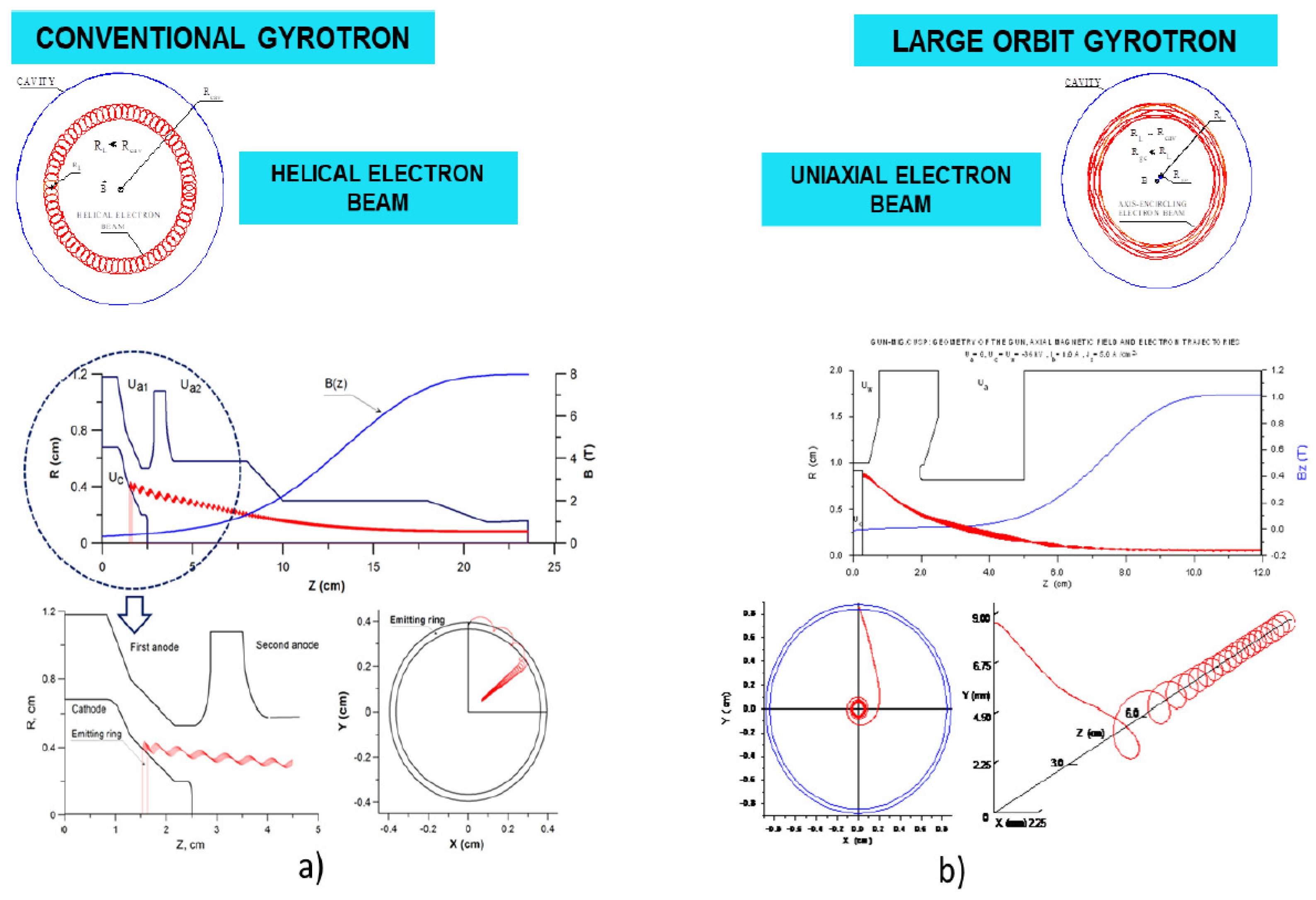
The invariants considered in this section form the basis for the widely used adiabatic theory of EOS for various gyro-devices (see, e.g., [18,69,70,71,72,73]), which is usually applied in the first (initial) stage of design considerations for the tube, before employing more sophisticated and adequate physical models. As an example, Figure 17 shows the results of the trajectory analysis of EOS for conventional and LOG, obtained using the ray-tracing codes GUN-MIG and GUN-MIG/CUSP of the problem-oriented package GYROSIM [22].

4. Conclusions

The theory of gyro-devices comprises a hierarchy of physical models (analytical, linear, nonlinear, time-independent (static), time-dependent, and self-consistent physical models), culminating in the first-principles formulations (based on Maxwell equations and the relativistic dynamics of electrons in time-varying electromagnetic fields) used in advanced numerical particle-in-cell (PIC) codes.

Over the years, these physical models have been implemented by many researchers from the gyrotron community in numerous stand-alone computer programs and software packages. We refer the reader to some of the most advanced and specialized numerical codes [74,75,76,77,78,79,80,81,82,83]. In addition to CAD (computer-aided design) and optimization, these problem-oriented software packages are also used for numerical studies of the gyro-devices and for educational purposes. Our experience shows that analyzing the results of numerical experiments performed with different physical models is very informative for understanding the underlying theory. Most of these modeling and simulation tools are in-house made codes that allow their users (who are also their developers) to modify the computational modules, input and output format, content, etc., as needed. However, some researchers (especially younger ones) nowadays prefer to use commercially available multiphysics software packages. We strongly discourage this, as we consider these to be, albeit powerful, “black boxes” (aka “number crunching machines”) that cannot be modified. Based on our experience, we believe that one of the best ways to study physics (including gyrotron theory) is to program the physical models yourself. In any case, knowing the basics presented in this paper will facilitate the interpretation of the results of the numerical experiments.

Although these fundamentals can be found scattered in numerous publications and monographs, they are not treated consistently and in sufficient detail. This was the main motivation for revisiting the most essential relations of gyrotron physics in an attempt (based on our teaching experience) to present them comprehensively in one place and in a proper order. We have endeavored to write a comprehensible, self-contained text that is understandable without resorting to additional sources. In this respect, the used carefully selected references should be considered mostly as suggestions for further reading for a more in-depth study of the discussed topics. We believe that the compendium of relationships and formulas presented here is essential for such studies and is aimed at the broad community of researchers working on the development and application of various gyro-devices. Furthermore, we hope that the material presented here in a pedagogical discourse will be a helpful advanced introduction to the physics of such devices.

References

- Gaponov-Grekhov, A.V.; Granatstein, V. Applications of High-Power Microwaves. In High-Power Microwave Electronics: A Survey of Achievements and Opportunities; Artech House Publishers: Norwood, MA, USA, 1994; Chapter 1. [Google Scholar]
- Nusinovich, G.; Thumm, M.; Petelin, M. The Gyrotron at 50: Historical Overview. J. Infrared Millim. Terahertz Waves 2014, 35, 325. [Google Scholar] [CrossRef]
- Petelin, M.I. The gyrotron: Physical genealogy. Terahertz Sci. Technol. 2015, 8, 157. [Google Scholar] [CrossRef]
- Petelin, M. The First Decade of the Gyrotronics. J. Infrared Millim. Terahertz Waves 2017, 38, 1387. [Google Scholar] [CrossRef]
- Plinski, E.F. Gorki’s Heroes. Bull. Pol. Acad. Sci. Tech. Sci. 2020, 68, 1259. [Google Scholar] [CrossRef]
- Thumm, M. State-of-the-Art of High-Power Gyro-Devices and Free Electron Masers. J. Infrared Millim. Terahertz Waves 2020, 41, 1–140. [Google Scholar] [CrossRef]
- Temkin, R. Development of terahertz gyrotrons for spectroscopy at MIT. Terahertz Sci. Technol. 2014, 7, 1–9. [Google Scholar] [CrossRef]
- Kumar, N.; Singh, U.; Bera, A.; Sinha, A. A review on the sub-THz/THz gyrotrons. Infrared Phys. Technol. 2016, 76, 38. [Google Scholar] [CrossRef]
- Glyavin, M.; Sabchevski, S.; Idehara, T.; Mitsudo, S. Gyrotron-Based Technological Systems for Material Processing-Current Status and Prospects. J. Infrared Millim. Terahertz Waves 2020, 41, 1022. [Google Scholar] [CrossRef]
- Idehara, T.; Sabchevski, S.; Glyavin, M.; Mitsudo, S. The Gyrotrons as Promising Radiation Sources for THz Sensing and Imaging. Appl. Sci. 2020, 10, 980. [Google Scholar] [CrossRef]
- Sabchevski, S.; Glyavin, M.; Mitsudo, S.; Tatematsu, Y.; Idehara, T. Novel and Emerging Applications of the Gyrotrons Worldwide: Current Status and Prospects. J. Infrared Millim. Terahertz Waves 2021, 42, 715. [Google Scholar] [CrossRef]
- Litvak, L.A.G.; Denisov, G.; Glyavin, M. Russian Gyrotrons: Achievements and Trends. IEEE J. Microwaves 2021, 1, 260. [Google Scholar] [CrossRef]
- Karmakar, S.; Mudiganti, J. Gyrotron: The Most Suitable Millimeter-Wave Source for Heating of Plasma in Tokamak. In Plasma Science and Technology; IntechOpen: London, UK, 2021. [Google Scholar] [CrossRef]
- Sabchevski, S.S.; Glyavin, M. Development and Application of THz Gyrotrons for Advanced Spectroscopic Methods. Photonics 2023, 10, 189. [Google Scholar] [CrossRef]
- Kartikeyan, M.; Borie, E.; Thumm, M. GYROTRONS High Power Microwave and Millimeter Wave Technology; Springer: Berlin/Heidelberg, Germany, 2003. [Google Scholar]
- Nusinovich, G. Introduction to the Physics of Gyrotrons; The Johns Hopkins University Press: Baltimore, MD, USA, 2004. [Google Scholar]
- Chu, K.R. The Electron Cyclotron Maser. Rev. Mod. Phys 2004, 76, 489. [Google Scholar] [CrossRef]
- Tsimring, S.E. Electron Beams and Microwave Vacuum Electronics; Wiley-Interscience: Hoboken, NJ, USA, 2007. [Google Scholar]
- Chao-Hai Du, P.K.L. Millimeter-Wave Gyrotron Traveling-Wave Tube Amplifiers; Springer: Berlin/Heidelberg, Germany, 2014. [Google Scholar]
- Gilmour, A.S. Klystrons, Traveling Wave Tubes, Magnetrons, Crossed-Field Amplifiers, and Gyrotrons; Artech House: Norwood, MA, USA, 2011. [Google Scholar]
- Grigoriev, A.D.; Ivanov, V.; Molokovsky, S. Microwave Electronics; Springer Series in Advanced Microelectronics; Springer: Berlin/Heidelberg, Germany, 2018; Volume 61. [Google Scholar] [CrossRef]
- Dattoli, G.; Palma, E.; Sabchevski, S.; Spassovsky, I. An overview of the gyrotron theory. In High Frequency Sources of Coherent Radiation for Fusion Plasmas; IOP Publishing: Bristol, UK, 2021; p. 51. [Google Scholar] [CrossRef]
- Siegman, A.E. Waves on a Filamentary Electron Beam in a Transverse-Field Slow-Wave Circuit. J. Appl. Phys. 1960, 31, 17. [Google Scholar] [CrossRef]
- Louisell, W.H. Coupled Mode and Parametric Electronics; John Wiley & Sons, Inc.: Hoboken, NJ, USA, 1960. [Google Scholar]
- Johnson, C.C. Theory of Fast-Wave Parametric Amplification. J. Appl. Phys. 1960, 31, 338. [Google Scholar] [CrossRef]
- Nusinovich, G.; Korol, M.; Jerby, E. Theory of the anomalous Doppler cyclotron-resonance-maser amplifier with tapered parameters. Phys. Rev. E 1999, 59, 2311. [Google Scholar] [CrossRef]
- Aitken, P.; McNeil, B.W.J.; Robb, G.R.M.; Phelps, A.D.R. Pulse propagation effects in a cyclotron resonance maser Amplifier. Phys. Rev. E 1999, 59, 1152. [Google Scholar] [CrossRef]
- Sabchevski, S.P.; Idehara, T. A numerical study on finite-bandwidth resonances of high-order axial modes (HOAM) in a gyrotron cavity. J. Infrared Millim. Terahertz Waves 2015, 36, 628. [Google Scholar] [CrossRef]
- Hornstein, M.K. Second harmonic operation at 460 GHz and broadband continuous frequency tuning of a gyrotron oscillator. IEEE Trans. Electron Devices 2005, 52, 798. [Google Scholar] [CrossRef]
- Chang, T.H.; Idehara, T.; Ogawa, I.; Agusu, L.; Kobayashi, S. Frequency tunable gyrotron using backward-wave components. J. Appl. Phys. 2009, 105, 063304. [Google Scholar] [CrossRef]
- Torrezan, A.C.; Shapiro, M.; Sirigiri, J.; Temkin, R.; Griffin, R. Operation of a Continuously Frequency-Tunable Second-Harmonic CW 330-GHz Gyrotron for Dynamic Nuclear Polarization. IEEE Trans. Electron Devices 2011, 58, 2777. [Google Scholar] [CrossRef]
- Barnes, A.B.; Nanni, E.; Herzfeld, J.; Griffin, R.J.; Temkin, R. A 250 GHz gyrotron with a 3 GHz tuning bandwidth for dynamic nuclear polarization. J. Magn. Reson. 2012, 221, 147. [Google Scholar] [CrossRef] [PubMed]
- Ikeda, R.; Yamaguchi, Y.; Tatematsu, Y.; Idehara, T.; Ogawa, I.; Saito, T.; Matsuki, Y.; Fujiwara, T. Broadband Continuously Frequency Tunable Gyrotron for 600MHz DNP-NMR Spectroscopy. Plasma Fusion Res. Rapid Commun. 2014, 9, 1206058. [Google Scholar] [CrossRef]
- Qi, C.H.D.; Liu, P.K. Broadband Continuous Frequency Tuning in a Terahertz Gyrotron with Tapered Cavity. Trans. Electron Devices 2015, 62, 4278. [Google Scholar] [CrossRef]
- Gao, Z.; Du, C.; Li, F.; Zhang, Z.; Li, S.; K, P. Forward-wave enhanced radiation in the terahertz electron cyclotron maser. Chin. Phys. B 2022, 31, 128401. [Google Scholar] [CrossRef]
- Sabchevski, S.; Glyavin, M.; Nusinovich, G. The Progress in the Studies of Mode Interaction in Gyrotrons. J. Infrared Millim. Terahertz Waves 2022, 43, 1–47. [Google Scholar] [CrossRef]
- Davydovskli, V.Y. On the possibility of accelerating charged particles by electromagnetic waves in a constant magnetic field. Zh. Eksp. Teor. Fiz 1962, 43, 886. [Google Scholar]
- Kolomenskii, A.A.; Lebedev, A. The autoresonance motion of a particle in a plane electromagnetic wave. Doklady Akad Nauk USSR 1962, 145, 1259–1261. [Google Scholar]
- Petelin, M.I. On the theory of ultrarelativistic cyclotron self-resonance masers. Radiophys. Quantum Electron. 1974, 17, 686. [Google Scholar] [CrossRef]
- Bratman, V.; Ginzburg, N.; Nusinovich, G.; Petelin, M.; Strklkov, P. Relativistic gyrotrons and cyclotron autoresonance masers. Int. J. Electron. Theor. Exp. 1981, 51, 541. [Google Scholar] [CrossRef]
- Danly, B.; Davies, J.; Pendergast, K.; Temkin, R.; Wurtele, J. High-frequency cyclotron autoresonance maser amplifier experiments at MIT. Microw. Part. Beam Sources Dir. Energy Concepts 1989, 1061, 243. [Google Scholar] [CrossRef]
- Bratman, V.; Denisov, G.; Kol’chugln, B.; Samsonov, S.; Volkov, A. Experimental demonstration of high-efficiency cyclotron-autoresonance maser operation. Rev. Lett. 1995, 75, 3102. [Google Scholar] [CrossRef] [PubMed]
- Cooke, S.J.; Cross, A.; He, W.; Phelps, A. Experimental operation of a cyclotron autoresonance maser oscillator at the second harmonic. Phys. Rev. Lett. 1996, 77, 4836. [Google Scholar] [CrossRef] [PubMed]
- Mirizzi, F. A high frequency, high power CARM proposal for the DEMO ECRH system. Fusion Eng. Des. 2015, 96, 538. [Google Scholar] [CrossRef]
- Vorob’ev, A.A.; Didenko, A.; Ishkov, A.; Kolomenskii, A.; Lebedev, A.; Yushkov, Y.G. Study of an autoresonance method of accelerating particles by electromagnetic waves. Sov. At. Energy 1967, 22, 1–4. [Google Scholar] [CrossRef]
- Golovanivsky, K.S. The Gyromagnetic Autoresonance. IEEE Trans. Plasma Sci. 1983, 11, 35. [Google Scholar] [CrossRef]
- Hafizi, B.; Sprangle, P.; Hirshfield, J. Electron beam quality in a cyclotron autoresonance accelerator. Phys. Rev. E 1994, 50, 3077. [Google Scholar] [CrossRef] [PubMed]
- LaPointe, M.A.; Yoder, R.B.; Wang, C.; Ganguly, A.; Hirshfield, J. Experimental Demonstration of High-Efficiency Cyclotron Autoresonance Acceleration. Phys. Rev. Lett. 1996, 76, 2718. [Google Scholar] [CrossRef] [PubMed]
- Shchelkunov, S.V.; Chang, X.; Hirshfield, J. Compact cyclotron resonance high-power accelerator for electrons. Phys. Rev. Accel. Beams 2022, 25, 021301. [Google Scholar] [CrossRef]
- Milant’ev, V. Cyclotron autoresonance and its Applications. Physics-Uspekhi 1997, 40, 1063. [Google Scholar] [CrossRef]
- Milant’ev, V. Cyclotron autoresonance—50 years since its discovery. Physics-Uspekhi 2013, 56, 1063. [Google Scholar] [CrossRef]
- Vomvoridis, J.L. An efficient Doppler-shifted electron-cyclotron maser oscillator. Int. J. Electron. 1982, 53, 555. [Google Scholar] [CrossRef]
- Fliflet, A. Linear and non-linear theory of the Doppler-shifted cyclotron resonance maser based on TE and TM waveguide Modes. Int. J. Electron. 1986, 61, 1049. [Google Scholar] [CrossRef]
- Fliflet, A.; McCowan, R.; Dullivan, C.; Kirkpatrick, D.; Gold, S. Development of high-power CARM oscillators. Nucl. Instrum. Methods Phys. Res. 1989, A285, 233. [Google Scholar] [CrossRef]
- Chen, C.; Wurtele, J. Linear and nonlinear theory of cyclotron autoresonance masers with multiple waveguide modes. Phys. Fluids Plasma Phys. 1991, 3, 2133. [Google Scholar] [CrossRef]
- Alberti, S.; Danly, B.; Gulotta, G.; Giguet, E.; Kimura, T.; Menninger, W.; Rullier, J.; Temkin, R. Experimental study of a 28 GHz high-power long-pulse cyclotron autoresonance maser oscillator. Phys. Rev. Lett. 2018, 71, 2018. [Google Scholar] [CrossRef] [PubMed]
- Nusinovich, G.; Latham, P.; Li, H. Efficiency of frequency up-shifted gyrodevices: Cyclotron harmonics versus CARM’s. IEEE Trans. Plasma Sci. 1994, 22, 796. [Google Scholar] [CrossRef]
- Dattoli, G.; Palma, E. The Cyclotron Auto-Resonance Maser: Analytical and numerical study. Nucl. Instrum. Methods Phys. Res. Sect. Accel. Spectrometers Detect. Assoc. Equip. 2020, 955, 163310. [Google Scholar] [CrossRef]
- Palma, E.; Dattoli, G.; Sabia, E.; Sabchevski, S.; Spassovsky, I. Beam–Wave Interaction From FEL to CARM and Associated Scaling Laws. IEEE Trans. Electron Devices 2017, 64, 4279. [Google Scholar] [CrossRef]
- Sabchevski, S.; Idehara, T. Cyclotron autoresonance with TE and TM guided waves. Int. J. Infrared Millim. Waves 2005, 26, 669. [Google Scholar] [CrossRef]
- Lawson, W.; Destler, W.; Striffler, C. High power microwave generation from a large orbit gyrotron. IEEE Trans. Nucl. Sci. 1985, 32, 2960. [Google Scholar] [CrossRef]
- Nusinovich, G. Non-linear theory of a large-orbit gyrotron. Int. J. Electron. 1992, 72, 959. [Google Scholar] [CrossRef]
- Bratman, V.; Kalynov, Y.; Fedotov, A. Theory of gyro devices with thin electron beams (large-orbit gyrotrons). Tech. Phys. 1998, 43, 1219. [Google Scholar] [CrossRef]
- Sabchevski, S.; Idehara, T.; Ogawa, I.; Glyavin, M.; Mitsudo, S.; Ohashi, K.; Kobayashi, H. Computer simulation of axis-encircling beams generated by an electron gun with a permanent magnet system. Int. J. Infrared Millim. Waves 2000, 21, 1191. [Google Scholar] [CrossRef]
- Kirstein, P.T.; Kino, G.; Waters, W. Space Charge Flow; McGraw-Hill Inc.: New York, NY, USA, 1967; p. 14. [Google Scholar]
- Chojnacki, E.; Destler, W.; Lawson, W.; Namkung, W. Studies of microwave radiation from a low-energy rotating electron beam in a multiresonator magnetron cavity. J. Appl. Phys. 1987, 61, 1268. [Google Scholar] [CrossRef]
- Rhee, M.J.; Destler, W.W. Relativistic electron dynamics in a cusped magnetic field. Phys. Fluids 1974, 17, 1574. [Google Scholar] [CrossRef]
- Destler, W.W.; Rhee, M. Radial and axial compression of a hollow electron beam using an asymmetric magnetic cusp. Phys. Fluids 1977, 20, 1582. [Google Scholar] [CrossRef]
- Gol’denberg, G.A.L.; Petelin, M. The formation of helical electron beams in an adiabatic gun. Radiophys. Quantum Electron. 1973, 16, 106. [Google Scholar] [CrossRef]
- Manuilov, V.N.; Tsimring, E. Synthesis of axially-symmetric systems for formation of helical electron beams. Radiotekhnika Elektron. 1978, 23, 1486. [Google Scholar]
- Shengpei, L. A method based on a simplified model for design of the gyrotron gun. J. Electron. 1984, 61, 192. [Google Scholar] [CrossRef]
- Baird, M.; Lawson, J. Magnetron injection gun (MIG) design for gyrotron applications. Int. J. Electron. Theor. Exp. 1986, 61, 953. [Google Scholar] [CrossRef]
- Molokovsky, S.; Sushkov, A. Intense Electron and Ion Beams; Springer: Berlin/Heidelberg, Germany; New York, NY, USA, 2005. [Google Scholar]
- Tarakanov, V. Code KARAT in simulations of power microwave sources including Cherenkov plasma devices, vircators, orotron, E-field sensor, calorimeter etc. EPJ Web Conf. 2017, 149, 04024. [Google Scholar] [CrossRef]
- Goplen, B.; Ludeking, L.; Smithe, D.; Warren, G. User-configurable MAGIC for electromagnetic PIC calculations. Comput. Phys. Commun. 1995, 87, 54. [Google Scholar] [CrossRef]
- Nguyen, T. Modeling of gyroklystrons with MAGY. IEEE Trans. Plasma Sci. 2000, 28, 867. [Google Scholar] [CrossRef]
- Jain, R.; Kartikeyan, M. Design of a 60 GHz, 100 kW CW gyrotron for plasma diagnostics: GDS V.01 simulations. Prog. Electromagn. Res. B 2010, 22, 379. [Google Scholar] [CrossRef]
- Sabchevski, S.; Zhelyazkov, I.; Thumm, M.; Illy, S.; Piosczyk, B.; Tran, T.; Hogge, J.; Pagonakis, J.G. Recent evolution of the simulation tools for computer aided design of electron-optical systems for powerful gyrotrons. Comput. Model. Eng. Sci. 2007, 20, 203. [Google Scholar] [CrossRef]
- Sabchevski, S.; Idehara, T.; Saito, T.; Ogaw, I.; Mitsudo, S.; Tatematsu, Y. Physical Models and Computer Codes of the GYROSIM (GYROtron SIMulation) Software Package; FIR Center Report FIR FU-99; University of Fukui: Fukui, Japan, 2010. [Google Scholar]
- Braunmueller, F.; Tran, T.; Vuillemin, Q.; Alberti, S.; Genoud, J.; Hogge, J.P.; Tran, M. TWANG-PIC, a novel gyro-averaged one-dimensional particle-in-cell code for interpretation of gyrotron experiments. Phys. Plasmas 2015, 22, 063115. [Google Scholar] [CrossRef]
- Wang, P.; Chen, X.; Xiao, H.; Dumbrajs, O.; Qi, X.; Li, L. GYROCOMPU: Toolbox Designed for the Analysis of Gyrotron Resonators. IEEE Trans. Plasma Sci. 2020, 48, 3007. [Google Scholar] [CrossRef]
- Sawant, A.; Choi, E. Development of the Full Package of Gyrotron Simulation Code. J. Korean Phys. Soc. 2018, 73, 1750. [Google Scholar] [CrossRef]
- Botton, M.; Antonsen, T., Jr.; Levush, B.; Nguyen, K.; Vlasov, A. MAGY: A Time-Dependent Code for Simulations of Slow and Fast Microwave Sources. IEEE Trans. Plasma Sci. 1998, 26, 882. [Google Scholar] [CrossRef]
Figure 1.
Structure and main parts of a gyrotron (modified from https://archive.org/details/gyrotron, accessed on 15 April 2024).
Figure 2.
Dispersion diagram of a hollow smooth-wall metallic waveguide.
Figure 3.
Dispersion characteristics of fast and slow transverse cyclotron waves in beams of electrons gyrating with cyclotron frequency .
Figure 4.
Normalized phase velocity ( of slow and fast cyclotron waves.
Figure 5.
Brillouin diagram of the beam–wave synchronism at resonance.
Figure 6.
Brillouin diagram at grazing condition.
Figure 7.
Normalized frequencies at the lower and higher intersection points of the Brillouin diagram vs. the magnetic field normalized to its value at grazing condition. This illustrative example is plotted for electron beam parameters .
Figure 8.
Brillouin diagram for the case of gyro-backward wave interaction.
Figure 9.
Discrete spectrum of the resonances (left plot) and schematic representation of the concept of finite-bandwidth resonances of HOAM in a gyrotron cavity (right plot).
Figure 10.
The variety of possible resonances in a gyrotron cavity with a dense spectrum of modes.
Figure 11.
Bundle of beam lines and their intersection with the dispersion curve of the cavity mode at cyclotron autoresonance.
Figure 12.
Types of helical electron beams used in gyro-devices: (a) polihelical electron beam of a conventional gyrotron; (b) uniaxial (axis-encircling) electron beam of a large orbit gyrotron. (—cavity radius, —guiding center radius, —Larmor radius).
Figure 13.
Nominator of the coupling factor G for different values of .
Figure 14.
On the conservation of the angular momentum and formulation of Busch’s theorem: forces acting on one electron.
Figure 15.
Schematic of the kinematics of a gyrating electron.
Figure 16.
Configuration of the magnetic field and electron orbits in an ideal (a) and in a realistic (b) cusp.
Figure 17.
Trajectory analysis of EOS in conventional and LOG. Trajectory analysis of EOS in conventional (a) and LOG (b). Reprinted with the permission of IOP Publishing from Ref. [22].
Disclaimer/Publisher’s Note: The statements, opinions and data contained in all publications are solely those of the individual author(s) and contributor(s) and not of MDPI and/or the editor(s). MDPI and/or the editor(s) disclaim responsibility for any injury to people or property resulting from any ideas, methods, instructions or products referred to in the content. |
© 2024 by the author. Licensee MDPI, Basel, Switzerland. This article is an open access article distributed under the terms and conditions of the Creative Commons Attribution (CC BY) license (https://creativecommons.org/licenses/by/4.0/).
Share and Cite
MDPI and ACS Style
Sabchevski, S. Fundamentals of Electron Cyclotron Resonance and Cyclotron Autoresonance in Gyro-Devices: A Comprehensive Review of Theory. Appl. Sci. 2024, 14, 3443. https://doi.org/10.3390/app14083443
AMA Style
Sabchevski S. Fundamentals of Electron Cyclotron Resonance and Cyclotron Autoresonance in Gyro-Devices: A Comprehensive Review of Theory. Applied Sciences. 2024; 14(8):3443. https://doi.org/10.3390/app14083443
Chicago/Turabian StyleSabchevski, Svilen. 2024. "Fundamentals of Electron Cyclotron Resonance and Cyclotron Autoresonance in Gyro-Devices: A Comprehensive Review of Theory" Applied Sciences 14, no. 8: 3443. https://doi.org/10.3390/app14083443
Note that from the first issue of 2016, this journal uses article numbers instead of page numbers. See further details here.