
Fault-Coping Algorithm for Improving Leader–Follower Swarm-Control Algorithm of Unmanned Surface Vehicles

1
Maritime ICT R&D Center, Korea Institute of Ocean Science & Technology, Busan 49111, Republic of Korea
2
Ocean Science & Technology School, Korea Maritime & Ocean University, Busan 49112, Republic of Korea
3
Marine Security and Safety Research Center, Korea Institute of Ocean Science & Technology, Busan 49111, Republic of Korea
4
Department of Mechanical Engineering, Korea Maritime & Ocean University, Busan 49112, Republic of Korea
5
Vessel Operation & Observation Team, Korea Institute of Ocean Science & Technology, Busan 49111, Republic of Korea
*
Author to whom correspondence should be addressed.
Appl. Sci. 2024, 14(8), 3444; https://doi.org/10.3390/app14083444
Submission received: 14 March 2024
/
Revised: 1 April 2024
/
Accepted: 18 April 2024
/
Published: 19 April 2024
(This article belongs to the Special Issue Selected Papers from the 12th International Multi-Conference on Engineering and Technology Innovation (IMETI 2023))
Abstract
:This study presents a swarm-control algorithm to overcome the limitations inherent to single-object systems. The leader–follower swarm-control method was selected for its ease of mathematical interpretation and theoretical potential for the unlimited expansion of followers. However, a known drawback of this method is the risk of swarm collapse when the leader breaks down. To address this, a fault-coping algorithm was developed and supplemented to the leader–follower swarm-control method, which enabled the detection and responsive handling of failures, thereby ensuring mission continuity. Comprehensive data, including voltage, current, thruster speed, position, and heading angle were acquired and analyzed using sensors on unmanned surface vehicles (USVs) to monitor potential failures. In the case of a failure, such as thruster malfunction, the nearest USV seamlessly takes charge of the mission under the guidance of the fault-coping algorithm. The leader–follower swarm-control and fault-coping algorithms were successfully validated through actual sea area tests, which confirmed their operational efficacy. This study affirms the well-formed nature of the USV swarm formation and demonstrates the effectiveness of the fault-coping algorithm in ensuring normal mission performance under the virtual failure scenarios applied to the leader USV.
1. Introduction
Multiagent systems with swarm control have broader utility in missions, such as for exploration or environmental characterization, than single-agent systems. Additionally, because the former employs multiple agents simultaneously, it exhibits an enhanced performance, shorter mission window, and increased cost efficiency and energy savings [1,2,3,4]. Existing research broadly classifies swarm-control methods into behavior-based swarm control, virtual-structure swarm control, and leader–follower swarm control [5]. According to studies [6,7,8], behavior-based swarm control has advantages such as minimal communication loss between unmanned vehicles and ease of establishing control power when multiple tasks are assigned. However, it is noted that behavior-based swarm control faces challenges in terms of mathematically representing control algorithms and maintaining desired swarm formation. Virtual-structure swarm control has the advantage of not requiring multiple rules or behaviors and making it easy to mathematically represent the behavior of the entire swarm formation. However, it is noted that to maintain swarm formation, wide-band communication is necessary, and significant computing power is required for path generation. Lastly, leader–follower swarm control offers advantages such as ease of mathematical representation and comprehension of swarm control algorithms, as well as easy implementation of algorithms. Theoretically, it is possible to expand the number of followers infinitely. However, a critical drawback is that the failure of the leader can lead to severe issues across the entire swarm formation. This limitation becomes prominent in marine environments with numerous environmental variables and a high probability of thruster system failure due to floating debris.
Therefore, in this study, we address the shortcomings of leader–follower swarm control by monitoring the state of unmanned surface vehicles (USVs) using various sensors. To handle an event of a failure, we propose a fault-coping algorithm that enables follower entities to assume the leader’s role and continue their missions. In addition, we developed a USV encoded with a leader–follower swarm-control algorithm. Through experiments in actual maritime regions, we verified its performance and confirmed the activation and functioning of the fault-coping algorithm during malfunctions.
2. Mathematical Modeling of Unmanned Surface Vehicle (USV)
2.1. Kinematics of USV
Figure 1 and Table 1 summarize the coordinate system of the developed USV and its vector and scalar notations per the definitions provided by the Society of Naval Architects and Marine Engineers, respectively.
The coordinate system of the USV employs earth- and body-fixed coordinates. However, because the earth- and body-fixed coordinates represent motion variables in different directions within the coordinate system, the expression of these motion variables based on the two coordinate systems must be transformed into a rotating coordinate system using rotation matrices.
Equation (1) represents the transformation matrix for converting the linear velocity observed in the body-fixed coordinate system to the linear velocity in the north–east–down (NED) coordinate system.
Equation (2) represents the transformation matrix for converting the angular velocity observed in the body-fixed coordinate system into that of the NED coordinate system.
Hence, the kinematic matrix representation of the USV is expressed in the form of Equation (3).
In this context, represents the position of the USV expressed in NED coordinates from the perspective of the earth-fixed coordinate system, where signifies the Euler angles representing the orientation between the earth-fixed and body-fixed coordinates. denotes the linear velocity of the USV in the body-fixed coordinate system with respect to the earth-fixed coordinate system. represents the angular velocity of the USV in the body-fixed coordinate system relative to the earth-fixed coordinate system. Detailed definitions of the parameters and conditions for Equations (1)–(3) are available in [9].
2.2. Modeling of USV Dynamics
The rigid-body dynamics of the USV were modeled based on Newton–Euler equations and vectorial–matrix dynamics. In this case, the USV underwent translational motion along the X and Y axes and rotational motion about the Z axis, constituting a three-degrees-of-freedom (3-DoF) platform. Therefore, the modeling process excluded the roll, pitch, and heave motions. According to “Guidance and Control of Ocean Vehicles”, the rigid-body dynamics equations of the USV can be expressed in the form of Equation (4) [10].
where represents the mass and inertia matrix of the USV, denotes the Coriolis and centripetal force matrix, and represents the external forces due to the USV’s propulsion system. The representation expressed in (4) is applicable to idealized scenarios such as simulation environments. However, for a more realistic representation, definitions related to hydrodynamic forces must be incorporated into the rigid-body dynamic equations.
As previously described, the USV undergoes 3-DoF motion, thereby eliminating the roll, pitch, and heave terms. The inertial matrix and Coriolis and centripetal forces resulting from the added mass are expressed in (5).
The damping matrix includes the fluid damping forces that depend on the relative velocity between the fluid and the USV. However, determination of the coefficients of fluid forces that exhibit nonlinear viscous relationships has limitations in terms of accuracy. Therefore, with the assumption that the influence of the damping forces beyond the second order is negligible, the total damping forces can be expressed as the sum of the linear and nonlinear damping forces, as indicated in (6) and (7).
where and represent the linear and nonlinear damping forces, respectively. By adding the inertia and Coriolis matrices obtained through the above derivations, along with the inertia and Coriolis matrices generated by the added mass, and subsequently adding the damping matrix, the rigid-body dynamics equation can be expressed as shown in (8).
where represents the components of force and moment acting on the USV from external factors such as waves, wind, and currents. However, because expressing each environmental variable mathematically was cumbersome, they were assumed to be absent. Therefore, by summing up all the terms on the left-hand side of (8) and expressing them in the form of a rigid-body dynamics equation, the rigid-body dynamics equation of the USV can be derived as in Equations (9)–(11):
where represents the thrust generated by the thruster system of the USV. Definitions of the parameters and conditions for the above equations are available in [11].
Finally, the forces and moments applied to the USV developed in this study were generated using two thruster units mounted on the port and starboard sides of the hull. The thruster units used in this case were not of the azimuth type and did not possess a separate rudder. Therefore, the control force and moment exerted by the thruster units on the USV are expressed as (12).
where and represent the propulsive forces exerted by the port and starboard thruster units of the USV, respectively, and D denotes the distance between them.
3. System Structure of USV
3.1. Communication System of USV
The two approaches to acquire data from unmanned vehicles in the leader–follower swarm-control method are the centralized and decentralized methods [12]. The centralized method is easier to implement in a swarm-control algorithm than the decentralized method. However, it requires substantial infrastructure, such as a server room, and an immobile ground control station. However, the decentralized method is marginally more complex to implement in a swarm-control algorithm than the centralized method. However, it offers the advantages of lower communication overhead, shorter information-sharing time among unmanned vehicles, and flexibility in not requiring a fixed ground control station [13]. Therefore, in this study, a leader–follower swarm-control method was implemented using the decentralized method. Figure 2 illustrates the communication circuit between the ground control station and the leader and follower USVs.
Communication between the ground control station and each USV was established via wireless RF TCP/IP equipment known as an access point (AP) bridge. The control inputs transmitted from the ground control station were relayed to each USV via the AP Bridge. The transmitted commands were segregated and delivered to the respective components within the USV through a switch hub installed on the board. Each component had a unique IP address to prevent conflicts among the information transmitted from the ground control station and ensure stable operation.
3.2. Sensor System of the USV
The USV was equipped with an inertial navigation system (INS) module, which comprised a GNSS and two L2-grade antennas for navigation. Additionally, it featured an RPM detector, a coulometer, and a reverse electromotive force-detection circuit for fault diagnosis. Furthermore, a camera sensor enabled the user to respond to emergencies (such as the sudden appearance of obstacles or collisions due to navigation algorithm errors) and survey mission areas.
The INS module outputs the current position (latitude and longitude) and heading data of the USV. The module’s data follow the National Marine Electronics Association (NMEA) 0183 format, with the position data using “GPRMC” and heading data using “GPHDT”. For more precise data, the module was equipped with the capability to simultaneously acquire GPS and GNSS satellite signals, enabling the interpolation of each satellite’s data.
In this study, fault diagnosis of a USV was performed by acquiring power consumption and thruster RPM data. Equations (13) and (14) represent the thruster torque. Equation (13) calculates the torque based on the output of the rotational speed of the thruster in RPM, while (14) represents the relationship between the voltage and current input to the thruster [14].
In (13), P represents the output of the thruster, N denotes the rotational speed of the thruster in RPM. In (14), p represents the pole pairs of the thruster, z is the number of conductors in the thruster, is the parallel circuit number of the thruster, is the flux in the thruster, and represents the current input to the thrusters. According to these equations, the torque of the thruster is inversely proportional to the rotational speed and directly proportional to the current. Therefore, fault diagnosis for the USV can be performed by detecting and comparing the rotational speed and current values.
A camera was installed to allow the user to monitor the real-time mission status of the USV. To enable the user to identify unexpected obstacles (such as reefs and other vessels) that may suddenly appear along the course of the USV, a wide-angle camera with a broad field of view was selected. Additionally, to ensure visibility during nighttime or in dark environments while conducting missions, a camera with infrared capabilities was mounted. This setup enabled the user to confirm and take actions, such as emergency stops or course correction, in response to unforeseen obstacles in the USV mission path.
4. Control Algorithm
4.1. Leader–Follower Swarm-Control Algorithm
Determination of goal formation between USVs is crucial for leader–follower swarm control. The primary motivation for researching swarm control of USVs in this study was that it enabled the use of multiple entities in missions, such as underwater surface exploration in the target area using an imaging sonar [15,16]. The utilization of multiple entities for exploration is advantageous in terms of time, energy, and efficiency. However, if the swarm formation is nonlinear, i.e., it morphs into different shapes, post-processing steps may be required after the mission. Therefore, a linear formation is preferred for exploratory missions as it helps streamline subsequent data processing and other procedures after mission completion.
Therefore, in this study, a formation control that can theoretically generate a linear swarm formation was employed as the swarm-formation controller. However, platforms operating in the marine environment, regardless of the sensitivity of the designed controller, may experience slower thruster responses due to various coefficients between water and air, such as fluid viscosity and friction coefficients. Consequently, if the swarm controller is used directly, maintaining a linear relationship between the leader and the followers becomes impractical.
To address this issue, in this study, a virtual point based on the leader USV and another virtual point based on the target point (waypoint) were trialed to generate the mission trajectory for the follower USVs. The virtual point based on the leader USV was employed to maintain a constant distance between the leader and its followers, while the one based on a waypoint was used to create the mission trajectory for the follower USVs. Figure 3 illustrates a schematic depicting the relationship among the leader, follower, and generated virtual points.
4.1.1. Virtual Point Based on Leader USV
The error in the distance between the leader and the followers was considered the control value. When the distance between the USVs exceeded a certain threshold, the leader would decelerate. When this distance decreases, it would revert to the original speed. This approach enhanced the stability of the swarm formation.
According to [17,18,19], the equation of error in the distance between the follower and the virtual point is given by (15).
where and represent the positions of the virtual points that are intended for the follower USV to follow. Using (15) and the non-holonomic dynamic model, the equation of error between the follower and the virtual point can be expressed in the forms of (16)–(18).
Similarly, the nonholonomic dynamic model in the form of Equations (16)–(18) can be condensed to (19)–(21), respectively.
where K is the speed control constant used to adjust the speed of the USV. Expanding (16)–(18) using (19)–(21), the equation for the leader’s speed control quantity is expressed as follows:
where represents the speed-control quantity of the leader USV, indicates the approach speed of the follower USV, denotes the angular velocity-control quantity of the leader USV, and represents the angular velocity of the follower USV.
4.1.2. Virtual Point Based on Waypoint
The virtual point generated based on the waypoint was used to create a trajectory that the follower should follow. When the virtual point was generated based on the leader’s target point, the distance errors for both the leader and follower USVs to reach the target point were similar. Therefore, if the controller weights of each USV were designed to be the same, the speed output for each USV to reach the target point would be similar, allowing for a linear formation.
To effectively maintain a linear formation, a control algorithm that considers the rotational situation, as depicted in Figure 4, is necessary.
In this study, to design a swarm controller that could effectively maintain the swarm formation considering rotational situations, the “exact formation control” method proposed in [20] was employed. Equation (23) represents the expression for exact formation control.
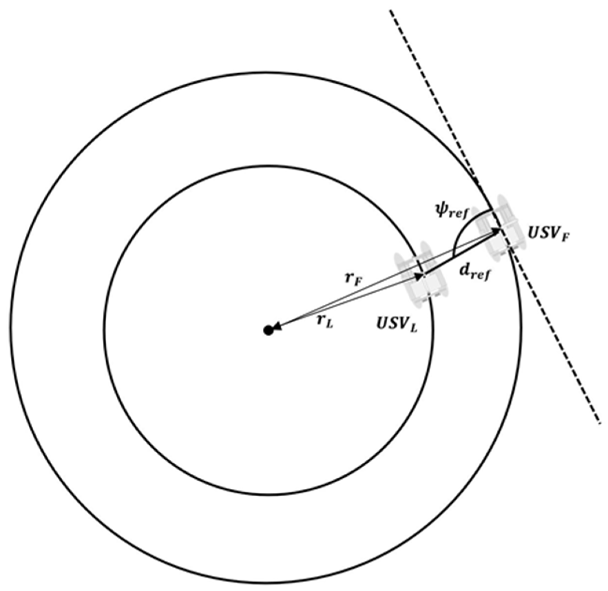
where and represent the linear velocities of the follower and leader USVs, respectively, and denotes the difference between the heading angles of the leader and follower USVs. Additionally, represents the target heading angle of the leader USV. The relationship between the turning radius of each USV and the formation control can be described as in Figure 5.
To maintain a linear formation, the follower must move along a circle with radius , and it should move faster than the leader along the circle. To achieve this, the relationship between the turning radii of the leader and follower is expressed as follows:
where represents the straight-line distance between a point on the turning radius of the leader and a point on the turning radius of the follower. denotes the angle between and the turning radius of the follower. Rearranging (24) in terms of and simplifying it using a quadratic formula gives (25):
The sign in front of the square root leads to both negative and positive values of the turning radius of the follower. A negative value indicates a linear formation where the leader’s turning radius is smaller than that of the follower, implying that the follower is positioned on the right-hand side of the leader. In contrast, a positive value indicates a linear formation in which the leader’s turning radius is greater than that of the follower, placing the follower to the left-hand side of the leader.
Finally, the turning radii of the leader and follower USVs are given by and , respectively. To maintain linear formation, must be equal to . Therefore, the speed control input for the follower can be expressed as indicated in (26).
Thus, utilizing the speed control input derived from (26) in the error term of the follower’s swarm controller allows for sustained formation control between the leader and the follower even as they turn. Detailed definitions of the control algorithm that considers rotational scenarios can be found in related studies [21,22].
4.2. Fault-Coping Algorithm
The major drawback of the leader–follower swarm-control method is that, if a fault occurs with the leader, the swarm cannot maintain its overall formation. To overcome this limitation, a fault-coping algorithm was applied in this study to bolster swarm control. The specific fault scenario considered in this study is a situation in which foreign substances are trapped in the thruster, leading to thruster malfunction. This is a common occurrence in marine platforms [23].
In this scenario, the overall system’s current consumption increases due to the fluid resistance load of the foreign material in the thruster.
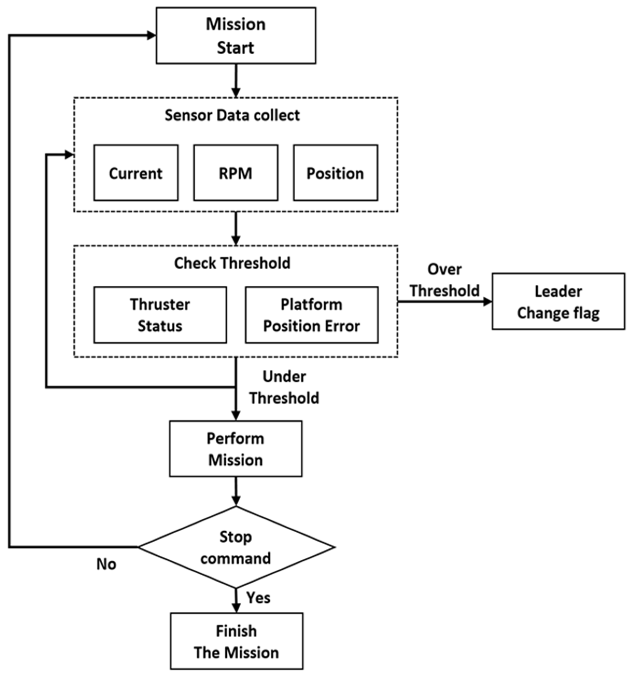
Consequently, the rotational speed of the thruster decreases. Subsequently, as the foreign material blocks the thruster’s drive shaft, the current diverges to the stall current value, and the thruster’s rotational motion is forcibly halted. Consequently, unintended motion in a direction different from that of the platform’s target motion occurs, making it impossible to maintain the swarm formation. Figure 6 illustrates a block diagram of the proposed fault-coping algorithm.
The fault-coping algorithm operates as follows: First, when the mission starts, sensors mounted on the USV acquire data such as the overall current consumption, rotational speed of the thruster in RPM, and position information of the USV.
Subsequently, the acquired data are input into the ‘Check Threshold Block’ to determine whether the state of data is more or less than the threshold value. A state of data similar to or less than the threshold value is considered normal, and the mission proceeds. During this time, the mission is repeated until a termination command is received from the user.
If the value of the acquired data is greater than the threshold value, it is considered a fault state, and the ‘Leader Change Flag’ is raised. Consequently, the USV experiencing the fault terminates the system, and among the USVs that are currently not experiencing a fault, it transfers its authority and mission to the one that is the closest in distance.
In the fault-coping algorithm, the check threshold block, which receives sensor data and determines their state, combines the ‘Thruster Status Block’, which identifies faults by comparing the values of the current, voltage, and RPM applied to the thruster to the threshold values, with the ‘Platform Position Error Block,’ which determines faults by comparing the current platform position, orientation, and heading data to the threshold values. Figure 7 depicts the thruster status block.
The thruster status block determines faults based on the applied current, voltage, and thruster RPM. When a foreign object is trapped in the thruster and hinders its normal operation, the current applied to the system increases, and the RPM value decreases or is not detected. The system detects such conditions through internally mounted components, such as a coulometer and a reverse power detection circuit and uses this information to identify fault scenarios.
In the thruster status block, the error used to determine the faults was calculated by subtracting the actual system current, voltage, and RPM values detected from the target current, voltage, and RPM values input to both thrusters. If the error did not exceed the threshold value, the system was considered normal. If the error exceeded the threshold, it was classified as a fault.
To prevent false positives because of noise or similar problems, the threshold for the thruster status block was designed to require a sustained error larger than the threshold for at least 3 s for the state to qualify as a faulty one. The threshold was determined based on experimental considerations by referencing the results of previous studies [24,25,26]. These studies observed through experiments that, in situations where foreign objects, such as ropes or seaweed, were entangled in the thruster, the current value increased by more than 4–50% compared with the input value, and the RPM value consistently decreased. Therefore, the threshold criterion in the thruster status block of this study was set to 1.5 times the input value. Figure 8 represents the platform position error block.
The platform position error block assesses faults based on data such as the current position, heading angle, and bearing angle of the USV. During a malfunction, such as due to interference in the thruster from foreign objects, the distance error between the USV and the target location may not decrease or the USV may deviate from the intended trajectory, leading to a divergence in the error values between the current position, heading angle, and target location. These outcomes were detected using sensors and used to determine the occurrence of a fault.
In this block, the error used to determine faults is the difference between the target cross-track error (CTE) value and the computed actual CTE value, as well as the difference between the target and actual heading angles detected by the sensors on the USV. Similar with the thruster status block, if the error value did not exceed a threshold, the system was considered normal. If the error value exceeded the threshold, it was considered a fault. To prevent the misinterpretation of transient errors caused by disturbances as faults, the threshold must persist for more than 3 s to be considered a fault. The threshold value in this block was set empirically with a CTE greater than 2 m and a heading angle greater than 10° as the fault criteria.
5. Experiments in Actual Maritime Area
The performances of the leader–follower swarm-control and fault-coping algorithms were tested in the maritime areas of Busan, South Korea. During the experiments, the maritime conditions were provided by the National Institute of Fisheries Science and were characterized by a wave height of 0.5–1 m, swell height of 0.6 m, and swell period of 8 s, which correspond to Sea State 3 [27]. Figure 9 illustrates a satellite image of the study area.
5.1. Leader–Follower Swarm-Control Algorithm Performance Test
The performance test of the leader–follower swarm-control algorithm involved placing the leader and follower USVs at different locations and heading angles. Next, four arbitrary waypoint locations were input, and the swarm controller, as discussed earlier, was evaluated for its proper operation, specifically verifying whether the follower successfully tracked the leader. Testing included analysis of the acquired data.
The results of the swarm control performance test, particularly the path-tracking outcome, are presented in Figure 10.
The results showed that, after initially being positioned in the upper-right corner of the leader, the follower executed a turn to organize a lateral formation. Subsequently, the follower maintained a consistent distance from the leader while navigating through each waypoint. As was observed, particularly at waypoints 3 and 4, the leader marginally deviated from the intended path due to a northeastward current during the experiment. This deviation resulted in an increase in the turning radii of both the leader and follower. Despite errors, the follower successfully maintained a constant distance from the leader.
The results of the swarm control performance test, specifically with respect to the heading angle, are presented in Figure 11.
The results indicate that, as shown in the graph, the leader and follower USVs, initially facing different angles, commenced and completed the mission with similar patterns. In this case, because the swarm formation involves a follower positioned to the right of the leader in a linear formation, the turning radius of the follower is larger than that of the leader. Consequently, in the graph, it is evident that the slope of the heading angle for the follower is gentler than that of the leader. Finally, Figure 12 illustrates the distance error between the leader and follower USVs.
The graph shows that the initial distance between the leader and the follower, which was approximately 12 m, was maintained at approximately 3.5 m during navigation. In each waypoint segment, the leader and follower turned, which caused the distance to increase by approximately 10 m. However, after the turning motion was completed, the distance was maintained at approximately 3–5 m during the navigation.
5.2. Fault-Coping Algorithm Performance Test
The performance of the fault-coping algorithm with the fault-coping algorithm was evaluated when unexpected changes in the current and RPM values of the developed USV occurred. The fault-coping algorithm successfully detected and assessed the fault, and the leader change flag was appropriately raised after the fault in the check threshold block was determined. The follower then assumed the role of the leader and continued the mission. Figure 13 shows a photograph of the actual fault situation that occurred during the test, and Figure 14 illustrates the path following results in the event of a fault.
These results are consistent with those of the swarm-control algorithm performance test. Initially, the follower USV, which was positioned behind the leader, successfully followed the leader at a constant distance from each waypoint. However, during the transition from waypoints 2 to 3, a fault occurred in the leader. Subsequently, the proposed fault-coping algorithm operated correctly, causing the leader to stop as the follower assumed the leader’s role. Finally, the follower successfully completed the mission by following the previous leader’s trajectory.
The current consumption and RPM data for the leader during the fault occurrence are depicted in Figure 15 and Figure 16, respectively.
As was evident from an examination of the graphs, approximately 150 s (1500 intervals in the figure) after the commencement of the mission, the current value increased by approximately 1.5 times from the previous value. Simultaneously, the thruster steadily decreased. This indicates that obstruction of the thruster by a foreign object caused a gradual reduction in the rotational speed and an increase in the overall power consumption of the system.
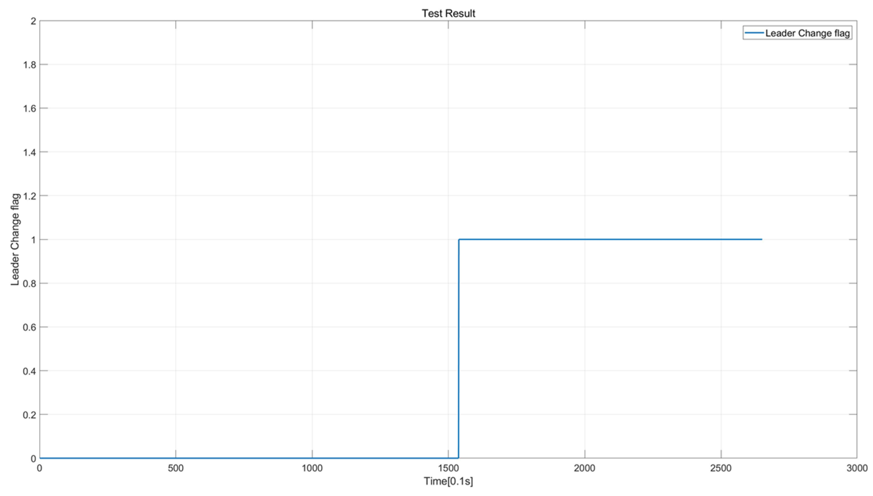
Subsequently, the fault-coping algorithm correctly identified the occurrence of a fault, leading to the cessation of the faulty USV system. Both the current and RPM values decreased to 0. Figure 17 illustrates the results, which confirm that the fault-coping algorithm accurately identifies the fault using current and RPM data, triggering the normal activation of the leader change flag.
As observed in Figure 15 and Figure 16, the leader change flag transitions from 0 to 1 simultaneously with the occurrence of the fault. These results verified that in a real operational environment, the proposed fault-coping algorithm would function accurately in unexpected fault scenarios during the mission.
6. Conclusions
In this study, we investigated a swarm-control algorithm to overcome the limitations of single-entity systems. We conducted research by selecting the leader–follower swarm-control method, which theoretically allows an infinite number of followers, to facilitate efficient exploration using USV in highly turbulent marine environments. This choice was made to enable easy system and algorithm development, as well as the effective exploration of vast maritime areas. To address the major drawback of this method, which is difficulty in maintaining the original formation in the event of a leader failure, we proposed a fault-coping algorithm capable of detecting leader failure and allowing a follower to spearhead the leader’s mission in the case of the latter’s failure. The performance of the proposed algorithms was verified via in situ experimentation.
For this research, we developed working USVs and equipped them with various sensors to monitor data in real time. In addition, we designed controllers for each USV using a separately developed swarm-control algorithm to enable the formation of the desired shape and achieve swarm control.
We assessed the performance of the designed controller by conducting a swarm-control performance test, where the leader and follower USVs formed the desired formation (maintaining a linear formation with the follower at 5 m to the starboard side of the leader) and tracked the target trajectory. During mission execution, we analyzed data from scenarios where faults occurred to confirm the functioning of the proposed fault-coping algorithm. It accurately detected the current and RPM values, determined faults based on these data, and successfully raised the leader change flag.
Finally, we confirmed that in the event of a fault in the leader USV, the follower USV successfully tracked the leader’s target path. Thus, this validates the performance of the proposed fault-coping algorithm.
Future research endeavors should aim to explore the proposed swarm-control algorithm with a large number of followers, enabling the implementation of a broader range of swarm formations beyond linear formations.
Additionally, in the context of the fault-coping algorithm, the investigation should be extended beyond the scenario addressed in this study (obstruction of the thruster by foreign objects). Algorithms capable of handling probable fault scenarios in marine environments, such as malfunctions due to seawater intrusion, damage resulting from collisions, and other relevant situations, should also be developed and validated.
Author Contributions
J.L. contributed to the conceptualization, methodology, and writing of the original draft. S.J. reviewed the corrections and formulae in the paper. H.C. analyzed the data. S.B. helped create the illustrations for this study. D.J. helped create the platform used in this study. All authors have read and agreed to the published version of the manuscript.
Funding
This research was part of a project titled “Development of smart maintenance monitoring techniques to prepare for disaster and deterioration of port infrastructure” funded by the Ministry of Oceans and Fisheries, Korea, Fund number: 20210659.
Institutional Review Board Statement
Not applicable.
Informed Consent Statement
Not applicable.
Data Availability Statement
The data supporting the conclusions of this article will be made available by the authors on request.
Acknowledgments
The authors would like to thank all the peer reviewers for their valuable contributions to this study.
Conflicts of Interest
The authors declare no conflicts of interest.
References
- Cruz, D.; Mcclintock, J.; Perteet, B.; Orqueda, A.A.O.; Cao, Y.; Fierro, R. Decentralized cooperative control—A multivehicle platform for research in networked embedded systems. IEEE Control Syst. 2007, 27, 58–78. [Google Scholar] [CrossRef]
- Feddema, J.T.; Lewis, C.; Schoenwald, D.A. Decentralized control of cooperative robotic vehicles: Theory and application. IEEE Trans. Robot. Autom. 2002, 18, 852–864. [Google Scholar] [CrossRef]
- Gu, Y.; Seanor, B.; Campa, G.; Napolitano, M.R.; Rowe, L.; Gururajan, S.; Wan, S. Design and flight testing evaluation of formation control laws. IEEE Trans. Control Syst. Technol. 2006, 14, 1105–1112. [Google Scholar] [CrossRef]
- Sallama, A.; Abbod, M.; Khan, S.M. Applying sequential particle swarm optimization algorithm to improve power generation quality. Int. J. Eng. Technol. Innov. 2014, 4, 223. [Google Scholar]
- Lee, K.R. Design of Decentralized Behavior-Based Network for the Formation Control and the Obstacle Avoidance of Multiple Robots. Ph.D. Thesis, Ajou University, Suwon-si, Republic of Korea, 2018. [Google Scholar]
- Park, S.B.; Park, J.H. A Study on Formation Control Algorithms of Multi-obstacles Collision Avoidance for Autonomous Navigation of Swarm Marine Unmanned Moving Vehicles. J. KNST 2020, 3, 56–61. [Google Scholar] [CrossRef]
- Lee, S.J.; Hong, S.K. Leader robot controller considering follower with input constraint. Trans. Korean Inst. Electr. Eng. 2012, 61, 1032–1040. [Google Scholar] [CrossRef]
- Tak, M.H.; Kim, J.S.; Joo, Y.H.; Ji, S.H. Formation Control for the Obstacle Avoidance of Swarm Robots Based Leader-Follower Robots; The Korean Institute of Electrical Engineers: Seoul, Republic of Korea, 2013; Volume 10, pp. 171–172. [Google Scholar]
- Wu, C.-J. 6-DoF Modelling and Control of a Remotely Operated Vehicle. Master’s Thesis, Flinders University, Adelaide, SA, Australia, 2018. [Google Scholar]
- Fossen, T.I. Guidance and Control of Ocean Vehicles; John Wiley & Sons: Hoboken, NJ, USA, 1994. [Google Scholar]
- Fossen, T.I. Handbook of Marine Craft Hydrodynamics and Motion Control; John Wiley & Sons: Hoboken, NJ, USA, 2011. [Google Scholar]
- Moon, S.T.; Lee, H.B.; Kim, P.J. Convergence research review. Converg. Res. Policy Cent. 2020, 6. [Google Scholar]
- Lawton, J.R.T.; Beard, R.W.; Young, B.J. A decentralized approach to formation maneuvers. IEEE Trans. Robot Auton. Syst. 2003, 55, 191–204. [Google Scholar] [CrossRef]
- Iwasaki, M.; Matusi, N. Robust speed control of IM with torque feed forward control. IEEE Trans. Ind. Electron. 1993, 40, 553–560. [Google Scholar] [CrossRef]
- Chen, Y.; Liu, Y.; Meng, S.Y.; Zhuang, Y. System modeling and simulation of an unmanned aerial underwater vehicle. J. Mar. Sci. Eng. 2019, 7, 444. [Google Scholar] [CrossRef]
- Rodriguez, J.; Castaneda, H.; Gordilo, J.L. Design of an adaptive sliding mode control for a micro-AUV subject to water currents and parametric uncertainties. J. Mar. Sci. Eng. 2019, 7, 445. [Google Scholar] [CrossRef]
- Dierks, T.; Jagannathan, S. Control of nonholonomic mobile robot formation: Back stepping kinematics into dynamics. In Proceedings of the IEEE Multi-Conference System Control, Suntec City, Singapore, 1–3 October 2007. [Google Scholar]
- Kanayama, Y.; Kimura, Y.; Miyazaki, F.; Noguchi, T. A stable tracking control method for an autonomous mobile robot. In Proceedings of the IEEE International Conference Robotics and Automation, Cincinnati, OH, USA, 13–18 May 1990. [Google Scholar] [CrossRef]
- Lee, S.J. Leader Robot Controller Considering Follower with Input Constraint. Master’s Thesis, Ajou University, Suwon-si, Republic of Korea, 2012. [Google Scholar]
- Consolini, L.; Morbidi, F.; Prattichizzo, D.; Tosques, M. Leader-follower formation control of nonholonomic mobile robots with input constraints. Automatica 2008, 44, 1343–1349. [Google Scholar] [CrossRef]
- Lee, J.H.; Jeong, S.K.; Ji, D.H.; Park, H.Y.; Kim, D.Y.; Choo, K.B.; Jung, D.W.; Kim, M.J.; Oh, M.H.; Choi, H.S. Unmanned surface vehicle using a leader-follower swarm control algorithm. Appl. Sci. 2023, 13, 3120. [Google Scholar] [CrossRef]
- Choi, I.S. Range Finder Based Leader-Follower Formation Control of Multiple Mobile Robot in Outdoor Environments. Master’s Thesis, Korea University, Seoul, Republic of Korea, 2013. [Google Scholar]
- Zanoli, S.M.; Astolfi, G.; Bruzzone, G.; Bibuli, M.; Caccia, M. Application of Fault Detection and Isolation Techniques on an Unmanned Surface Vehicle(USV). In Proceedings of the IFAC Conference on Maneuvering and Control of Marine Craft, Arenzano, Italy, 19–21 September 2012. [Google Scholar] [CrossRef]
- Cho, H.J.; Choi, H.S.; Kim, H.J.; Nam, K.S.; Ryu, J.D.; Ha, K.N. Feature selection for unmanned surface vehicle fault diagnosis research and experimental verification. J. Inst. Control. Robot. Syst. 2022, 28, 542–550. [Google Scholar] [CrossRef]
- Choo, K.B.; Cho, H.J.; Park, J.H.; Huang, J.; Jung, D.W.; Lee, J.H.; Jeong, S.K.; Yoon, J.S.; Choo, J.H.; Choi, H.S. A research on fault diagnosis of a USV thruster based on PCA and entropy. Appl. Sci. 2023, 13, 3344. [Google Scholar] [CrossRef]
- Kim, M.J.; Cho, H.J.; Choo, K.B.; Huang, J.; Jung, K.W.; Park, J.H.; Lee, J.H.; Jeong, S.K.; Ji, D.H.; Choi, H.S. Design of Underwater Thruster Fault Detection Model Based on Vibration Sensor Data: Generative Adversarial Network-Based Fault Data Expansion Approach for Data Imbalance. Sens. Mater. 2022, 34, 3213–3227. [Google Scholar] [CrossRef]
- Korea Real Time Database for NEAR-GOOS. Available online: http://www.khoa.go.kr/oceangrid/koofs/eng/observation/obs_real.do (accessed on 20 July 2021).
Figure 1.
Coordinates of unmanned surface vehicle (USV).

Figure 2.
Schematic of the communication system between the leader and follower USVs.

Figure 3.
Relationship diagram of leader–follower USVs and virtual points.

Figure 4.
Rotational situation of leader–follower swarm control.

Figure 5.
Relationship between the turning radius and formation control.

Figure 6.
Block diagram of fault-coping algorithm.

Figure 7.
Thruster status block.

Figure 8.
Platform position error block.

Figure 9.
Satellite picture of experimental area.

Figure 10.
Path following the results of the swarm control performance test.

Figure 11.
Heading angle results of swarm control performance test.

Figure 12.
Distance error result of swarm-control performance test.

Figure 13.
Picture of actual fault scenario.

Figure 14.
Path following result of fault scenario.

Figure 15.
Current data of fault scenario.

Figure 16.
RPM data of fault scenario.

Figure 17.
Leader change flag result of fault scenario.


Table 1.
Notation of the Society of Naval Architects and Marine Engineers (SNAME) for the unmanned surface vehicle (USV).
Table 1.
Notation of the Society of Naval Architects and Marine Engineers (SNAME) for the unmanned surface vehicle (USV).
| Force and Moments | Linear and Angular Velocities | Position and Euler Angle | |
|---|---|---|---|
| Motion in the X direction (surge) | X | u | x |
| Motion in the Y direction (sway) | Y | v | y |
| Motion in the Z direction (heave) | Z | w | z |
| Rotation about the X axis (roll) | K | p | |
| Rotation about the Y axis (pitch) | M | q | |
| Rotation about the Z axis (yaw) | N | r |
Disclaimer/Publisher’s Note: The statements, opinions and data contained in all publications are solely those of the individual author(s) and contributor(s) and not of MDPI and/or the editor(s). MDPI and/or the editor(s) disclaim responsibility for any injury to people or property resulting from any ideas, methods, instructions or products referred to in the content. |
© 2024 by the authors. Licensee MDPI, Basel, Switzerland. This article is an open access article distributed under the terms and conditions of the Creative Commons Attribution (CC BY) license (https://creativecommons.org/licenses/by/4.0/).
Share and Cite
MDPI and ACS Style
Lee, J.; Ji, D.; Cho, H.; Baeg, S.; Jeong, S. Fault-Coping Algorithm for Improving Leader–Follower Swarm-Control Algorithm of Unmanned Surface Vehicles. Appl. Sci. 2024, 14, 3444. https://doi.org/10.3390/app14083444
AMA Style
Lee J, Ji D, Cho H, Baeg S, Jeong S. Fault-Coping Algorithm for Improving Leader–Follower Swarm-Control Algorithm of Unmanned Surface Vehicles. Applied Sciences. 2024; 14(8):3444. https://doi.org/10.3390/app14083444
Chicago/Turabian StyleLee, Jihyeong, Daehyeong Ji, Hyunjoon Cho, Saehun Baeg, and Sangki Jeong. 2024. "Fault-Coping Algorithm for Improving Leader–Follower Swarm-Control Algorithm of Unmanned Surface Vehicles" Applied Sciences 14, no. 8: 3444. https://doi.org/10.3390/app14083444
Note that from the first issue of 2016, this journal uses article numbers instead of page numbers. See further details here.