A Dynamic Parameter Tuning Strategy for Decomposition-Based Multi-Objective Evolutionary Algorithms

Abstract

The penalty-based boundary cross-aggregation (PBI) method is a common decomposition method of the MOEA/D algorithm, but the strategy of using a fixed penalty parameter in the boundary cross-aggregation function affects the convergence of the populations to a certain extent and is not conducive to the maintenance of the diversity of boundary solutions. To address the above problems, this paper proposes a penalty boundary crossing strategy (DPA) for MOEA/D to adaptively adjust the penalty parameter. The strategy adjusts the penalty parameter values according to the state of uniform distribution of solutions around the weight vectors in the current iteration period, thus helping the optimization process to balance convergence and diversity. In the experimental part, we tested the MOEA/D-DPA algorithm with several MOEA/D improved algorithms on the classical test set. The results show that the MOEA/D with the DPA has better performance than the MOEA/D with the other decomposition strategies.

1. Introduction

Many real-life problems involve conflicting and interdependent objectives. The challenge is to optimize multiple objectives simultaneously within a given region, which is known as a multi-objective optimization problem. Multi-objective optimization problems are very important and highly researched in real life, such as in engineering applications, including coil spring design problems for commercial three-wheeled vehicles [1], solar photovoltaic forecasting [2], wind energy forecasting and research issues [3], air pollution forecasting issues [4], aerodynamic design issues [5], etc. Yang and Jiang defined the multi-objective optimization problem as shown in Equation (1) [6]:

The decision space is represented by ${\mathsf{\Omega }}_{\mathrm{x}}\subseteq {\mathrm{R}}^{\mathrm{n}}$, while $n_h,n_g$ represent the number of equations and inequalities, respectively. The number of objectives is denoted by m, and ${F\left(x\right):\Omega }_x\to R^M$ is the objective function vector used to solve for x. Therefore, a multi-objective optimization problem typically yields a set of optimal solutions, known as the Pareto optimal solution set. In 1896, the scholar Pareto introduced the concept of the Pareto optimal solution. A domination is defined as follows: $\forall {\mathrm{f}}_{\mathrm{t}}\left({\mathrm{x}}_{\mathrm{i}}\right)\le {\mathrm{f}}_{\mathrm{t}}\left({\mathrm{x}}_{\mathrm{j}}\right)$ and $\exists {\mathrm{f}}_{\mathrm{t}}\left({\mathrm{x}}_{\mathrm{i}}\right)<{\mathrm{f}}_{\mathrm{t}}\left({\mathrm{x}}_{\mathrm{j}}\right)$, j = 1, 2, …, m, $x_i$ dominates $x_j$, denoted $x_i$ < $x_j$, and is referred to as Pareto domination. A solution is considered Pareto optimal if it is not dominated by any other solutions. The set of objective values corresponding to each solution in the Pareto solution set is known as the Pareto frontier [7].

Zhang and Li proposed the MOEA/D algorithm for decomposition-based multi-objective optimization in 2007 [8]. The approach adopted involves decomposition to address multi-objective problems. This is achieved by converting a multi-objective problem into multiple single-objective sub-problems that can be solved individually, and utilizing a neighborhood search strategy and weight vectors to ensure global convergence and diversity. Compared to other multi-objective optimization algorithms, such as the dominance-based multi-objective optimization algorithm (NSGA-II), MOEA/D has several advantages: the MOEA/D algorithm uses a decomposition strategy for solving, so it can effectively deal with high-dimensional problems [9,10,11]; approximation of Pareto optimal solutions by collaborative solving among subproblems [12,13]; and using a single reference point to guide solution generation reduces the number of depth evaluations and improves the efficiency of the algorithm by only evaluating the solution in the vicinity of the reference point in each problem [14,15,16].

$$\left\{\begin{array}{c}min\hspace{1em}F\left(x\right)={\left(f_1\right(x),f_2(x),\dots ,f_m(x\left)\right)}^T\hfill \\ s.t.\hspace{1em}{h}_i\left(x\right)=0,\hspace{1em}\hspace{1em}i=1,\dots ,n_h\hfill \\ g_i\left(x\right)\ge 0,\hspace{1em}\hspace{1em}i=1,\dots ,n_g\\ x\in {\Omega }_x\end{array}\right.$$

(1)

MOEA/D commonly uses three decomposition methods: the weighted sum method, the Tchebycheff approach, and the penalty-based boundary intersection method (PBI). The algorithm’s performance is affected by the number of weight vectors used in the weight summation approach [17], too few to adequately explore the various regions of the Pareto front, and too many, leading to an increase in terms of the algorithm’s computational complexity. Also, when the distribution of the weight vectors is not uniform [18], it may lead to the weight vectors being too dense or sparse in some regions, which affects the search ability of the algorithm. The Chebyshev aggregation approach has a large dependence on the weight vector [19], and the determination of the weights between the objective functions needs to be performed [20]. Also, when there are fewer objectives, the distribution of optimal solutions obtained by the Chebyshev aggregation approach is more scattered [21]. The PBI decomposition approach provides high search efficiency and optimization quality for interactability problems and nonlinear and nonconvex optimization problems [22]. The PBI decomposition approach has higher feasibility and validity for initial population individuals and better reflects the characteristics of the problem than the other two decompositions in MOEA/D [23]. In addition, the PBI decomposition approach allows for the selection of appropriate penalty parameters according to the needs of the specific problem [24]. This can result in a more effective adaptation of the generated population to the objective function and a quicker discovery of the globally optimal solution during the optimization process.

The size of the penalty parameter in the PBI algorithm significantly affects its convergence and diversity. In 2019, when solving hybrid energy system optimization problems [25], Guo, Yang, and Jiang first set the penalty parameter to 0.5, when the diversity of the algorithm was low, and then changed the value of the penalty parameter to 3.0 when the diversity of the algorithm was significantly increased. In 2015, in response to the multi-target backpack problem [26], Ishibuchi, Akedo, and Nojima found that the convergence rate for a penalty parameter value of 0.1 is significantly higher than that for a penalty parameter value of 5.0. The algorithm’s diversity increases with larger penalty parameter values, while smaller penalty parameter values increase its convergence [27,28,29]. Therefore, the value of the penalty parameter should be different depending on the problem; in contrast, in the traditional MOEA/D-PBI decomposition approach, the penalty parameter is usually designed as a fixed value. Fixed penalty parameters do not capture the characteristics of the problem well when dealing with problems of high complexity. Also, when there is a large conflict between the objective function value and the constraints, the two need to be balanced by adjusting the penalty parameter, and a fixed penalty parameter cannot flexibly cope with this trade-off problem.

To tackle the aforementioned situation, this paper suggests a novel penalty approach, namely the boundary-crossing strategy with dynamically adjusted penalization parameters (MOEA/D-DPA). MOEA/D-DPA adaptively adjusts the penalty parameter values according to the state of the uniform distribution of the solutions around the weight vectors for the iteration period currently in progress.

This paper is structured as follows: Section 2 explains the MOEA/D-PBI algorithm and the significance of the penalty factor in it. Section 3 proposes an improved penalization strategy for the PBI algorithm. Section 4 presents an experimental study of the proposed punishment strategy. Section 5 summarizes the research presented in this paper.

2. Related Work

2.1. MOEA/D-PBI

The decomposition-based multi-objective optimization algorithm (MOEA/D) employs three decomposition methods. This section will focus on the penalty-based boundary cross-aggregation approach (PBI) as an example to provide a detailed introduction to the MOEA/D algorithm process.

The input to the MOEA/D-PBI algorithm contains the following:

① Objective functions: Define multiple objective functions that need to be minimized or maximized; these functions are a measure of the performance of the optimization problem. ② Constraints: Define possible constraints. Constraints are problem limitations that need to be satisfied, e.g., feasibility, resource constraints, etc. ③ Weight vector: Determines the weights of each objective function in the optimization problem. ss④ Penalty factor: Gives the factor used to penalize the violation of constraints. Penalty factors are used to penalize solutions that do not meet the constraints and to motivate the algorithm to find a better solution if the constraints are met. ⑤ Algorithm parameters: Set the parameters required by the algorithm, including population size, crossover rate, mutation rate, etc., which will affect the speed of convergence and the final results of the algorithm.

Output of the MOEA/D-PBI algorithm:

① Approximate Pareto optimal solution set: These solutions perform relatively well on multiple objective functions and can no longer be improved by improving one objective function without compromising the others. These solutions are distributed on the Pareto front and represent the best trade-off solution to the problem. ② The objective function value for each solution: The MOEA/D-PBI algorithm provides the value of each objective function for every solution in the set of approximate Pareto optimal solutions. These values help us evaluate the performance of each solution on different objective functions. ③ Feasibility information: The MOEA/D-PBI algorithm also provides information on the feasibility of each solution. This indicates whether each solution satisfies the constraints. If the solution does not satisfy the constraints, the algorithm may apply a penalty factor to it to correct it.

The MOEA/D-PBI algorithm steps include the following:

① Initialization: Set the number of populations N and generate the initial population P(0) = {$x_1\left(0\right),x_2\left(0\right),\dots ,x_n\left(0\right)$}.

② Decoupling Decomposition: For each individual $x_{\left(i\right)}\left(t\right)\in$ P(t), compute its decomposition weight vector $\mathsf{\lambda }\left(\mathrm{i}\right)$ = (${\lambda }_1\left(i\right),{\lambda }_2\left(i\right),\dots ,{\lambda }_m\left(i\right)$, The variable ‘m’ represents the number of targets, while ‘i’ denotes the index of the individual.

③ Update the set of neighbors: For each individual $x_{\left(i\right)}\left(t\right)\in$ P(t), find its set of neighbors. The selection of the set of neighbors can be based on the distance metric or topology.

④ Evolutionary operations: For each individual $x_{\left(i\right)}\left(t\right)\in$ P(t), perform the following steps: (a) Select two parent individuals (x($p_1$),x($p_2$)) $\in {\mathrm{N}}_{\left(\mathrm{i}\right)}$. (b) Use crossover and mutation operations to generate a child individual x(off). (c) Compute the decomposition weight vector (off) for the child individuals. (d) Determine whether a child individual can replace a parent individual.

If $\mathsf{\lambda }$(off) is close to $\mathsf{\lambda }\left(\mathrm{i}\right)$, replace the parent individual. Otherwise, retain the parent individual.

⑤ Renewal of stocks: For each individual $x_{\left(i\right)}\left(t\right)\in$ P(t), it is updated according to the fitness value, which can be calculated using the Pareto boundary crossing (MOEA/D-PBI) function.

⑥ Termination judgment: Check whether the termination conditions are satisfied, such as reaching the preset number of iterations or the degree of convergence of the solution.

⑦ Produce an approximate set of Pareto-optimal solutions: Upon satisfaction of the termination condition, the algorithm outputs the approximate set of Pareto-optimal solutions.

2.2. Effect of Penalizing Factor θ on PBI

Jiang and Yang analyzed the effect of punishment factor θ on PBI [6]. Specifically, when a solution does not meet the conditions, the objective function value of the solution is penalized by the PBI algorithm through the addition of a penalty term, and the size of this penalty term has a penalty factor to determine. If the penalty factor is excessive, the algorithm will penalize solutions that fail to meet the constraints, which may cause the algorithm to favor solutions that satisfy the constraints and therefore increase the diversity of the algorithm. On the contrary, if the penalty factor is smaller, the algorithm penalizes less for solutions that do not meet the constraints, which may cause the algorithm to be more inclined to find better solutions, i.e., solutions that may not meet the constraints, and therefore improve the convergence of the algorithm.

Figure 1 and Figure 2 show the effect of two different values of the penalty parameter θ on convergence and diversity [6].

The penalty factor $\mathsf{\theta }$ is set to 1.0 in Figure 1; ${\mathsf{\omega }}_1={(0.1,0.9)}^{\mathrm{T}}$ and ${\mathsf{\omega }}_2={(0.2,0.8)}^{\mathrm{T}}$ denote two neighboring boundary weight vectors. From Figure 1, B and C are the optimal points of ${\mathsf{\omega }}_1,{\mathsf{\omega }}_2$, two boundary weight vectors, respectively. Since ${\mathrm{g}}^{\mathrm{p}\mathrm{b}\mathrm{i}}\left(\mathrm{B}|{\mathsf{\omega }}_1,{\mathrm{z}}^{\mathrm{*}}\right)$ = 0.60 is less than ${\mathrm{g}}^{\mathrm{p}\mathrm{b}\mathrm{i}}\left(\mathrm{B}|{\mathsf{\omega }}_1,{\mathrm{z}}^{\mathrm{*}}\right)$ = 0.75, the solution of the subproblem for ${\mathsf{\omega }}_1$ with the associated sub-problem is replaced by C from B. So, when the penalty factor is small, the algorithm may find more non-dominated solutions because it is easier for the algorithm to find solutions that do not meet the constraints but have smaller objective function values. These non-dominated solutions may cause congestion in the Pareto front and thus reduce the diversity of the algorithms. In Figure 2, since the penalty factor $\mathsf{\theta }$ is set to a large 5.0, H and J are the optimal points of the two boundary weight vectors of ${\mathsf{\omega }}_1,{\mathsf{\omega }}_2$, respectively, but since the ${\mathrm{g}}^{\mathrm{p}\mathrm{b}\mathrm{i}}$ of J is larger than that of H, H will not be replaced by J. So, when the penalty factor is large, the algorithm may find fewer non-dominated solutions because it focuses more on those solutions that satisfy the constraints. These solutions satisfying the constraints may be more decentralized, thus increasing the diversity of the algorithms.

And later in the paper [6], the adaptive penalization scheme (MOEA/D-APS) was proposed. MOEA/D-APS proposes adaptively adjusting the penalty factor $\mathsf{\theta }$ based on different search stages. In the early stage, the main optimization goal is to converge towards the real PF quickly, so the penalty factor $\mathsf{\theta }$ is set to a small value; In the subsequent stages, the penalty parameter is increasing, and at this point, the algorithm focuses more on the diversity of the population. APS uses this formula to achieve the above goals:

$$\theta ={\theta }_{min}+({\theta }_{max}-{\theta }_{min})\frac{it}{maxIteration}$$

(2)

The variable $\mathrm{i}\mathrm{t}$ represents the current number of iterations, while $\mathrm{m}\mathrm{a}\mathrm{x}\mathrm{I}\mathrm{t}\mathrm{e}\mathrm{r}\mathrm{a}\mathrm{t}\mathrm{i}\mathrm{o}\mathrm{n}$ represents the total number of population iterations. ${\mathsf{\theta }}_{\mathrm{m}\mathrm{i}\mathrm{n}}$ and ${\theta }_{max}$ represent the upper and lower bounds of $\mathsf{\theta }$, respectively, and $\theta$ takes the value 5.0; ${\mathsf{\theta }}_{\mathrm{m}\mathrm{i}\mathrm{n}}=1.0,{\mathsf{\theta }}_{\mathrm{m}\mathrm{a}\mathrm{x}}=10.0$.

3. Suggested Strategies for Improvement

3.1. Basic Concept

The aim of this paper is to tackle the issue that the penalty parameter is a fixed value in the traditional PBI decomposition method, which affects the convergence speed of the population to some extent, so we propose a boundary-crossing strategy to adaptively adjust the penalty parameter. The core idea of the dynamic tuning strategy is that the penalty parameter affects the probability of the offspring being retained to a certain extent, thus affecting the convergence and diversity of the population. According to the PBI formula, the larger the penalty parameter, the less likely the offspring will be retained. Therefore, at the start of each iteration, the primary objective is to bring the population as close as possible to the Pareto front, so it is necessary to make the penalty parameter low, a large number of substitution operations occur in the offspring, and population turnover; as the number of iterations increases, the penalty parameter is gradually increased, so that the population is diversified and dispersed. To cover the entire Pareto front, it is necessary to include all relevant options. Based on this approach, the penalty parameter is adaptively adjusted according to the current distribution of solutions around the weight vector. When the distribution of solutions around the weight vector is too wide, the penalty parameter decreases to increase the convergence of the population; when the distribution of solutions around the weight vector is too small, the penalty parameter increases to increase the diversity of the population.

3.2. Boundary-Crossing Strategy for Adaptive Tuning of Penalty Parameters

In this paper, adaptive parameter tuning is used to regulate the convergence and diversity of the population, thus accelerating population convergence. From the above analysis, it can be seen that the size of the penalty parameter $\mathsf{\theta }$ is inextricably related to the current iteration period. At the beginning of the iteration, the penalty parameter $\mathsf{\theta }$ is low, the population undergoes a large number of substitution operations, and the population convergence increases, rapidly approaching the Pareto frontier. In the later stages of the iteration, the penalty parameter value $\mathsf{\theta }$ rises and the population dispersion and diversity increase so that the population does not miss any part of the Pareto front. Therefore, this paper makes the following improvements based on Equation (2):

During the evolution of a population, if the penalty parameter $\theta$ is too small, the solutions at the frontier are easily replaced by solutions closer to the center, which results in a decrease in population diversity. If the penalty parameter $\mathsf{\theta }$ is too large, the occurrence of the replacement operation in the population is not frequent, which significantly impacts the convergence speed of the population and hinders its ability to approach the Pareto frontier effectively. As a result, the penalty parameter’s value is related to the current iteration period, as well as the uniformity of the current population distribution. Therefore, on the basis of the above tuning formula, the distribution density of the current population should be taken into account. Therefore, the uniform state of the subproblem is defined first:

$${avg}^i=\frac{{nc}^i-{nc}_{min}}{{nc}_{max}-{nc}_{min}}$$

(3)

Among them, ${\mathrm{a}\mathrm{v}\mathrm{g}}^{\mathrm{i}}\in \left[\mathrm{0,1}\right]$ is the uniform state of the distribution of solutions around the weight vector, the number of solutions to the weight vector is represented by ${\mathrm{n}\mathrm{c}}^{\mathrm{i}}$. The minimum number of solutions is represented by ${\mathrm{n}\mathrm{c}}_{\mathrm{m}\mathrm{i}\mathrm{n}}$, and ${\mathrm{n}\mathrm{c}}_{\mathrm{m}\mathrm{a}\mathrm{x}}$ represents the maximum number of solutions. For the solution $x^j$, if the distance between the vector and weight vector $\mathrm{i}$ is less than the distance between its corresponding solution ${\mathrm{x}}^{\mathrm{i}}$ and weight vector $\mathrm{i}$, it is considered to be distributed around weight vector $\mathrm{i}$, i.e.,

$${nc}^i=\left\{x^j\right|d\left(x^j,w^i\right)<d\left(x^i,w^i\right)\}$$

(4)

where $\mathrm{d}(\mathrm{x},\mathrm{w})$ denotes the perpendicular distance from the solution $x$ to the weight vector $w$, i.e.,

$$d\left(x,w\right)=\Vert \overline{F}\left(x\right)-\frac{w^T\overline{F}\left(x\right)}{w^{T}w}\Vert$$

(5)

where $\overline{\mathrm{F}}\left(\mathrm{x}\right)$ is the normalized processing function for solving $\mathrm{x}$, which is treated as in Equation (6).

$$ASF\left(x,w_j\right)={max}_{i=1}^m\left\{\frac{1}{w_{j,i}}\left|\frac{f_i\left(x\right)-z_i^{*}}{z_i^{nad}-z_i^{*}}\right|\right\}$$

(6)

Since the final population sought has to balance convergence and diversity, if there are too many solutions distributed around the weight vector, it is too convergent, and the current population is not evenly distributed. During population evolution, if the penalty parameter $\mathsf{\theta }$ is too small, solutions at the boundary are easily replaced by solutions closer to the center. If the penalty parameter $\mathsf{\theta }$ is too large, the population is less susceptible to replacement operations. Therefore, this paper proposes to further adjust the penalty parameter $\mathsf{\theta }$ according to the current solution distribution state on the basis of tuning the parameter according to the current iteration state. When there are too many solutions distributed around the current weight vector, the penalty parameter is decreased to increase the convergence of the solutions; when there are too few solutions distributed around the weight vector, the penalty parameter is increased to increase the population diversity.

$$\theta =\left\{\begin{array}{l}\mathit{max}\left\{{\theta }_{min},\frac{\theta }{2}\right\}\hspace{1em}\hspace{1em}if{avg}^i>0.4\\ \mathit{min}\left\{{\theta }_{max},\theta *2\right\} \hspace{1em}if{avg}^i\le 0.4\end{array}\right.$$

(7)

3.3. MOEA/D-DPA Algorithm

The MOEA/D-DPA algorithm is divided into five main steps: initialization, constructing the solution, selecting the children, updating the value of the penalty parameter $\mathsf{\theta }$, and updating the solution set in five parts. Its pseudo-algorithm is shown in Algorithm 1, and the algorithmic procedure is described in detail below.

In the first step, an initialization operation is performed. Generate N vectors uniformly distributed in a multidimensional space. Ensure that the vectors are uniformly distributed and calculate their Euclidean distance. The Euclidean distance for each vector to select its nearest T vectors will be counted in the order in the middle $\mathrm{B}\left(\mathrm{i}\right)$, $\mathrm{B}\left(\mathrm{i}\right)=\{{\mathrm{i}}_1,\dots ,{\mathrm{i}}_{\mathrm{T}}\}$, where this ${\mathrm{w}}^{\mathrm{i}1},\dots ,{\mathrm{w}}^{\mathrm{i}\mathrm{T}}$ that is ${\mathrm{w}}^{\mathrm{i}}$ distance nearest T vectors.

In the second step, an initial population $\mathrm{P}=\{{\mathrm{x}}^1,\dots ,{\mathrm{x}}^{\mathrm{N}}\}$ is generated from the solution space in a randomized manner. ${\mathrm{z}}_{\mathrm{i}}^{\mathrm{*}}$ and ${\mathrm{z}}^{\mathrm{n}\mathrm{a}\mathrm{d}}$ will be computed at the same time, where ${\mathrm{z}}_{\mathrm{i}}^{\mathrm{*}}$ is the ideal value, and precise computation will be very time consuming, so it will be estimated by the minimum value of the current population, which is constantly updated as the population iterates; similarly ${\mathrm{z}}_{\mathrm{i}}^{\mathrm{n}\mathrm{a}\mathrm{d}}$ of the minimum ${\mathrm{z}}^{\mathrm{n}\mathrm{a}\mathrm{d}}$ is estimated by the worst value achieved by the current population in the ${\mathrm{f}}_{\mathrm{i}}$ direction, and continuously updated.

The third step is to construct the solution. Constructing the solution in this algorithm is mainly divided into four parts, structured reference points, cross variation, normalization process, and clustering. The following algorithm outlines the steps to be taken.

In the fourth step, the population is updated. The strategy used is to choose to replace ${\mathrm{x}}^{\mathrm{j}}$ with a solution y if the resulting solution y is better than any of the solutions x in $\mathrm{B}\left(\mathrm{i}\right)$, i.e., ${\mathrm{g}}^{\mathrm{p}\mathrm{b}\mathrm{i}}\left(\mathrm{y}\right|{\mathrm{w}}^{\mathrm{j}},{\mathrm{z}}^{\mathrm{*}})\le {\mathrm{g}}^{\mathrm{p}\mathrm{b}\mathrm{i}}({\mathrm{x}}^{\mathrm{j}}|{\mathrm{w}}^{\mathrm{j}},{\mathrm{z}}^{\mathrm{*}})$, as judged by the PBI formula, this contributes to preserving the diversity of the population and gradually enhancing the quality of the solution.

In the fifth step, the value of the penalty parameter $\mathsf{\theta }$ is adaptively adjusted according to the PBI tuning formula introduced in this chapter.

Finally, keep repeating the above steps until the maximum number of iterations is reached.

Algorithm 1 $\mathbf{M}\mathbf{O}\mathbf{E}\mathbf{A}/\mathbf{D}-$DPA

Input: maxIteration: a stopping criterion; N: the quantity of subproblems evaluated in MOEA/D; a uniform spread of N weight vector: ${\lambda }^1\dots {\lambda }^N$; T: the number of weight vectors in the neighborhood of each weight vector. Output: EP 1: Initialization: Generate a uniform spread of N weight vectors: $w^1,\dots ,w^N$ and compute the T closest weight vectors to each weight vector by the distance. For each $i=1,\dots ,N$, set $B\left(i\right)=\{i_1,\dots ,i_T\}$ where $w^{i1},\dots ,w^{iT}$ are the T closest weight vectors to $w^i$. 2: Create the initial population P 3: While the stopping criteria have not been met, do: 4: Randomly select two indexes $r_{1}and{r}_{2}fromB\left(i\right)$ 3: Solution construction 4: Select construction 5: Determine the value of parameter $\theta$ 6: Update of EP 7: End while

3.4. Algorithm Complexity Analysis

From Algorithm 1, the computational cost of the MOEA/D-DPA algorithm is mainly within the iterations. Let the population size of the MOEA/D-DPA algorithm be m, the number of subproblems be N, and the number of weight vectors be T. Unlike the original MOEA/D algorithm, when updating, the MOEA/D-DPA algorithm must compute the current value of the penalty parameter. The algorithm has a time complexity of O(1), and the average time complexity to compute each generation is O(mNT).

The MOEA/D-DPA algorithm is considered to have similar time and space complexity to the original MOEA/D algorithm, as it does not require additional storage space. This ensures that the improved MOEA/D-DPA algorithm does not significantly alter the algorithm’s complexity.

4. Discussion

4.1. Compare Functions and Test Functions

To assess the efficacy of the algorithm proposed in this paper, the experimental part is run on ZDT and DTLZ test sets. The comparison algorithms are chosen: MOEA/D-AGG, MOEA/D-TCHE, MOEA/D-PBI, and the improved algorithms MOEA/D-SPS and MOEA/D-2PBI [30] for the PBI approach.

To ensure comparability among all algorithms, all the same parameters in the experiment were set to the same values. Let the number of neighbors T = 20, crossover probability $P_c$ = 0.2, and variance probability $P_m$ = 0.2. The population size is 200, and the maximum number of iterations is set to 25,000. All algorithms are run independently 25 times.

In this paper, four ZDT functions are selected as test functions, and their function expressions are shown in

Table 1. ZDT test function table.

Problem	Objective Functions	Variable Bounds
ZDT1	$MinF=\{f_1,f_2\}$ $f_1=x_1$ $f_2=g\times h$ $g=1+9\times {\displaystyle \sum _{i=2}^n}{x}_i/(n-1)$ $h(f_1,g)=1-\sqrt{f_1/g}$	$n=30$ $x_iϵ\left[\mathrm{0,1}\right]$
ZDT2	$MinF=\{f_1,f_2\}$ $f_1=x_1$ $f_2=g\times h$ $g=1+9\times {\displaystyle \sum _{i=2}^n}{x}_i/(n-1)$ $h(f_1,g)=1-{(f_1/g)}^2$	$n=30$ $x_iϵ\left[\mathrm{0,1}\right]$
ZDT3	$MinF=\{f_1,f_2\}$ $f_1=x_1$ $f_2=g\times h$ $g=1+9\times {\displaystyle \sum _{i=2}^n}{x}_i/(n-1)$ $h(f_1,g)=1-\sqrt{f_1/g}-(f_1/g)\times sin\left(10\pi f_1\right)$	$n=30$ $x_iϵ\left[\mathrm{0,1}\right]$
ZDT4	$MinF=\{f_1,f_2\}$ $f_1=x_1$ $f_2=g\times h$ $g=1+10\times (n-1)$ $+{\displaystyle \sum _{i=2}^n}(x_i^2-10cos(4\pi x_i\left)\right)$ $h(f_1,g)=1-\sqrt{f_1/g}$	$n=10$ $x_1ϵ\left[\mathrm{0,1}\right]$ $x_2,\dots ,x_nϵ[-\mathrm{5,5}]$

.

Since all ZDT test functions are bi-objective optimization problems, DTLZ is chosen as a set of three-objective optimization test functions, which can be set to have three objectives by considering the number of its objectives. Let be the human-set parameter, its function expression is shown in

Table 2. DTLZ test function table.

Problem	Objective Functions	Variable Bounds
DTLZ1	$MinF=\{f_1,f_2,f_3\}$ $f_1=(1+g)\times 0.5\times x_1{x}_2$ $f_2=(1+g)\times 0.5\times x_1(1-x_2)$ $f_3=(1+g)\times 0.5\times {(1-x}_1)$ $g=100[|x_m|+{\displaystyle \sum _{x_i\in x_M}}{(x_i-0.5)}^2-cos(20\pi (x_i-0.5))]$	$x_iϵ\left[\mathrm{0,1}\right]$
DTLZ2	$MinF=\{f_1,f_2,f_3\}$ $f_1=(1+g)cos(x_1\pi /2)cos(x_2\pi /2)$ $f_2=(1+g)cos(x_1\pi /2)sin(x_2\pi /2)$ $f_3=(1+g)sin(x_1\pi /2)$ $g={\displaystyle \sum _{x_i\in x_M}}{(x_i-0.5)}^2$	$x_iϵ\left[\mathrm{0,1}\right]$
DTLZ3	$MinF=\{f_1,f_2,f_3\}$ $f_1=(1+g)cos(x_1\pi /2)cos(x_2\pi /2)$ $f_2=(1+g)cos(x_1\pi /2)sin(x_1\pi /2)$ $f_3=(1+g)sin(x_1\pi /2)$ $g=100[|x_m|+{\displaystyle \sum _{x_i\in x_M}}{(x_i-0.5)}^2-cos(20\pi (x_i-0.5))]$	$x_iϵ\left[\mathrm{0,1}\right]$
DTLZ4	$MinF=\{f_1,f_2,f_3\}$ $f_1=(1+g)cos(x_1^{\alpha }\pi /2)cos(x_2^{\alpha }\pi /2)$ $f_2=(1+g)cos(x_1^{\alpha }\pi /2)sin(x_2^{\alpha }\pi /2)$ $f_3=(1+g)sin(x_1^{\alpha }\pi /2)$ $g={\displaystyle \sum _{x_i\in x_M}}{(x_i-0.5)}^2$	$x_iϵ\left[\mathrm{0,1}\right]$
DTLZ5	$\mathrm{M}\mathrm{i}\mathrm{n}\mathrm{F}=\{{\mathrm{f}}_1,{\mathrm{f}}_2,{\mathrm{f}}_3\}$ ${\mathrm{f}}_1=(1+\mathrm{g})\mathrm{c}\mathrm{o}\mathrm{s}({\mathsf{\theta }}_1\mathsf{\pi }/2)\mathrm{c}\mathrm{o}\mathrm{s}({\mathsf{\theta }}_2\mathsf{\pi }/2)$ ${\mathrm{f}}_2=(1+\mathrm{g})\mathrm{c}\mathrm{o}\mathrm{s}({\mathsf{\theta }}_1\mathsf{\pi }/2)\mathrm{s}\mathrm{i}\mathrm{n}({\mathsf{\theta }}_2\mathsf{\pi }/2)$ ${\mathrm{f}}_3=(1+\mathrm{g})\mathrm{s}\mathrm{i}\mathrm{n}({\mathsf{\theta }}_1\mathsf{\pi }/2)$ ${\mathsf{\theta }}_{\mathrm{i}}=\frac{\mathsf{\pi }}{4(1+\mathrm{g})}(1+2\mathrm{g}{\mathrm{x}}_{\mathrm{i}})$ $\mathrm{g}={\displaystyle \sum _{{\mathrm{x}}_{\mathrm{i}}\in {\mathrm{x}}_{\mathrm{M}}}}{({\mathrm{x}}_{\mathrm{i}}-0.5)}^2$	$x_iϵ\left[\mathrm{0,1}\right]$
DTLZ6	$MinF=\{f_1,f_2,f_3\}$ $f_1=(1+g)cos({\theta }_1\pi /2)cos({\theta }_2\pi /2)$ $f_2=(1+g)cos({\theta }_1\pi /2)sin({\theta }_2\pi /2)$ $f_3=(1+g)sin({\theta }_1\pi /2)$ ${\theta }_i=\frac{\pi }{4(1+g)}(1+2g{x}_i)$ $g={\displaystyle \sum _{x_i\in x_M}}{x}_i^{0.1}$	$x_iϵ\left[\mathrm{0,1}\right]$
DTLZ7	$MinF=\{f_1,f_2,f_3\}$ $f_1=x_1$ $f_2=x_2$ $f_3=x_3$	$x_iϵ\left[\mathrm{0,1}\right]$

.

4.2. Performance Indicators

This paper employs the inverted generational distance evaluation metric (IGD) and the hypervolume metric (HV) to evaluate multi-objective optimization algorithms.

The IGD value indicates the minimum distance from the population to the ideal Pareto front obtained by the algorithm, i.e., the smaller the value of IGD, the closer the population is to the ideal Pareto front and is distributed in each part of the Pareto front, the better the algorithm performs. Therefore, the IGD value can be a good assessment of the convergence and diversity of the algorithm.

Inverted generational distance (IGD):

$$IGD(P^{*},P)=\frac{{\sum }_{vϵP^{*}}d(v,P)}{\left|P^{*}\right|}$$

(8)

The function $d(v,P)$ represents the minimum Euclidean distance from the point v to P. The point P denotes the solution set of the algorithm to find the population. ${\mathrm{P}}^{*}$ is a set of uniformly distributed points obtained from the ideal Pareto front, and $\left|{\mathrm{P}}^{*}\right|$ is the size of ${\mathrm{P}}^{*}$.

The HV value is used to comprehensively evaluate the convergence and diversity of the solutions obtained by the multi-objective optimization algorithm. The larger the HV value, the closer the current population is considered to be to the ideal Pareto frontier. However, the choice of reference point needs to be more careful, because it will greatly affect the accuracy of the HV value.

Hypervolume (HV):

$$HV\left(X,P\right)=\bigcup _{xϵX}^{X}v(x,P)$$

(9)

In the set of non-occupied solutions $X$, $v(x,P)$ represents the hypervolume of the space formed by the solution $x$ and the reference point $P$. This is equivalent to the volume of the hypercube constructed with the line between the solution $x$ and the reference point $P$ as the diagonal.

4.3. Experimental Results and Analysis

4.3.1. Experimental Results

Figure 3 and Figure 4 show the distribution of the Pareto frontiers obtained by the four algorithms on the ZDT and DTLZ test problem sets. On the bi-objective problem, it can be seen from Figure 3 that on the ZDT1 problem, the populations obtained by the PBI and TCHE approaches can approach the Pareto frontier very well, and the distribution of the solutions obtained by the AGG and 2PBI approaches is poorer. The MOEA/D-TC and MOEA/D-SPS algorithms maintain the convergence and diversity quality of solutions obtained by the PBI approach, while also achieving a more uniform distribution of solutions. And the distribution of the solutions is more uniform. On the ZDT2 problem, the quality of the solutions obtained by the TC, PBI, and TCHE approaches is all better, and the MOEA/D-SPS and MOEA/D-2PBI algorithms perform slightly worse, where the distribution curves of the solutions obtained by the TC strategy are smoother and of higher quality when compared with the pre-improved PBI decomposition approach. On the test set ZDT3, the quality of the solutions obtained by the TC strategy is poor, while the quality of the solutions obtained by the TCHE decomposition approach is better. On the test problem ZDT4, the improved TC strategy is more improved than the original PBI decomposition, the obtained curve is smoother, and the population distribution is more uniform. From the distribution graph of the obtained solution set, it can be initially recognized that on the dual-objective problem, the improved TC strategy improves the solution quality to a certain extent.

On the triple-objective problem, as illustrated in Figure 4, the improved MOEA/D-TC algorithm yields Pareto that is more similar to the ideal Pareto frontier on the DTLZ2, DTLZ3, DTLZ5, and DTLZ6 test problems. The MOEA/D-TC algorithm performs poorly on the DTLZ1 and DTLZ7 test problems. On the DTLZ4 problem, both the MOEA/D-TC algorithm and the original MOEA/D-PBI algorithm can find the solution set better. Therefore, it can be preliminarily concluded that the MOEA/D-TC algorithm has some improvement over the MOEA/D-PBI decomposition strategy on the triple objective problem.

4.3.2. Analysis of IGD Performance Index Results

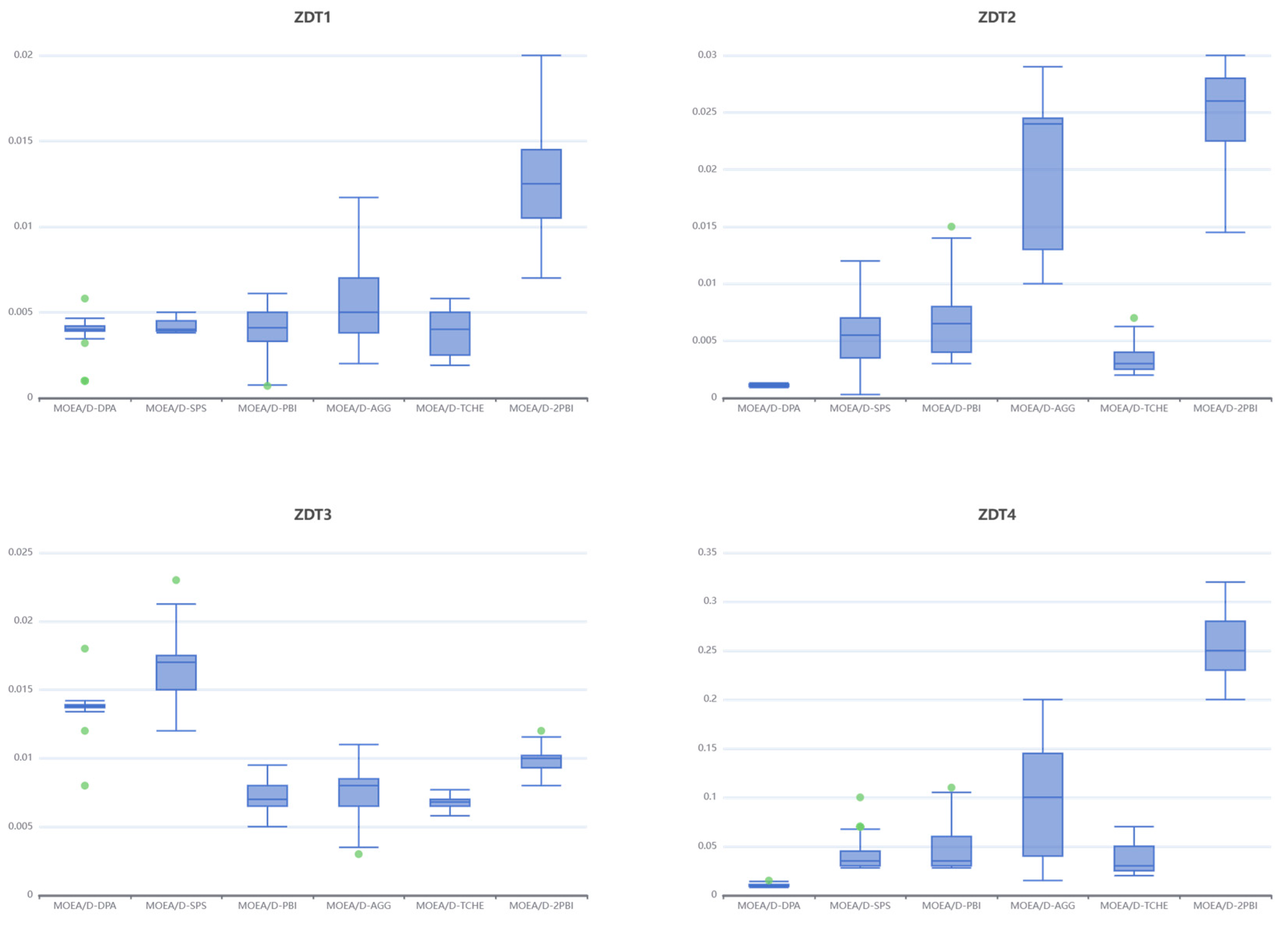
The mean, standard deviation, median, and quartiles for the IGDs of the algorithms MOEA/D-SPS, MOEA/D-PBI, MOEA/D-AGG, MOEA/D-TCHE, and MOEA/D-2PBI, and the algorithm MOEA/D-DPA proposed in this paper, are given in

Table 3. IGD mean and standard deviation of algorithms.

	MOEA/D-DPA	MOEA/D-SPS	MOEA/D-PBI	MOEA/D-AGG	MOEA/D-TCHE	MOEA/D-2PBI
ZDT1	4.30E-3 (1.5E-4)	4.30E-3 (6.7E-4)	7.70E-3 (3.6E-3)	1.12E-3 (6.4E-4)	2.78E-3 (1.1E-3)	1.23E-2 (3.1E-3)
ZDT2	5.77E-4 (3.7E-4)	4.71E-3 (1.8E-3)	1.14E-2 (6.2E-3)	1.32E-2 (3.2E-3)	3.06E-3 (1.4E-3)	2.21E-2 (4.6E-3)
ZDT3	8.98E-3 (1.7E-3)	1.57E-2 (2.7E-3)	1.42E-2 (1.1E-3)	4.15E-3 (1.8E-3)	6.84E-3 (7.9E-4)	9.85E-3 (1.0E-3)
ZDT4	8.43E-3 (4.8E-3)	3.69E-2 (3.1E-2)	9.35E-2 (5.9E-2)	3.86E-2 (1.9E-2)	4.79E-2 (3.0E-2)	5.48E-1 (1.6E-1)
DTLZ1	8.99E-4 (2.3E-5)	9.87E-4 (1.6E-4)	6.60E-4 (3.0E-4)	4.90E-3 (2.1E-5)	2.12E-2 (2.6E-2)	3.47E-2 (3.4E-2)
DTLZ2	3.55E-4 (1.3E-6)	6.29E-4 (1.4E-5)	7.61E-4 (2.0E-5)	5.35E-3 (1.5E-6)	7.74E-4 (1.1E-5)	1.08E-3 (6.5E-5)
DTLZ3	3.07E-3 (1.2E-2)	2.11E-2 (4.6E-2)	6.10E-2 (1.2E-1)	2.00E-2 (2.3E-2)	2.28E-1 (2.5E-1)	3.11E-1 (4.0E-1)
DTLZ4	1.03E-3 (8.7e-4)	1.42E-3 (9.5E-4)	1.24E-3 (2.1E-4)	5.88E-3 (1.0E-11)	1.32E-3 (2.7E-4)	1.69E-3 (2.7E-4)
DTLZ5	1.03E-3 (9.8E-6)	1.06E-3 (4.6E-5)	1.44E-3 (2.6E-5)	3.09E-2 (5.5E-10)	9.92E-4 (3.0E-5)	1.01E-3 (1.7E-4)
DTLZ6	1.56E-3 (2.7E-5)	1.78E-3 (7.5E-5)	1.78E-3 (7.5E-5)	4.65E-2 (1.9E-2)	4.25E-3 (9.4E-3)	7.42E-3 (2.1E-2)
DTLZ7	3.75E-2 (5.1E-3)	3.66E-2 (5.2E-3)	9.96E-3 (4.3E-4)	1.54E-2 (3.8E-3)	2.91E-3 (4.2E-3)	2.74E-2 (3.9E-3)

and

Table 4. IGD median and quartile of algorithms.

	MOEA/D-DPA	MOEA/D-SPS	MOEA/D-PBI	MOEA/D-AGG	MOEA/D-TCHE	MOEA/D-2PBI
ZDT1	4.27E-3 (2.3E-4)	4.08E-3 (8.7E-4)	7.02E-3 (7.2E-3)	9.09E-4 (6.3E-4)	2.57E-3 (1.7E-3)	1.22E-2 (4.4E-3)
ZDT2	4.72E-4 (4.2E-4)	4.36E-3 (3.3E-3)	1.07E-2 (9.2E-3)	1.30E-2 (1.1E-3)	2.91E-3 (2.2E-3)	2.21E-2 (8.0E-3)
ZDT3	1.37E-2 (1.4E-4)	1.73E-2 (5.5E-3)	8.71E-3 (2.8E-3)	3.77E-3 (3.0E-3)	6.78E-3 (1.0E-3)	9.88E-3 (1.1E-3)
ZDT4	6.75E-3 (6.5E-3)	3.01E-2 (2.7E-2)	3.01E-2 (2.7E-2)	3.64E-2 (2.7E-2)	3.75E-2 (3.9E-2)	5.19E-1 (2.7E-1)
DTLZ1	8.94E-4 (2.5E-5)	1.05E-3 (2.1E-4)	5.61E-4 (4.3E-5)	4.90E-3 (5.2E-9)	8.00E-3 (3.2E-2)	3.03E-2 (5.4E-2)
DTLZ2	3.55E-4 (2.6E-6)	6.32E-4 (2.3E-5)	7.62E-4 (2.6E-5)	5.35E-3 (2.1E-11)	7.73E-4 (1.2E-5)	1.08E-3 (7.8E-5)
DTLZ3	6.24E-4 (6.2E-5)	1.07E-3 (6.7E-3)	1.08E-2 (5.5E-2)	1.14E-2 (6.8E-3)	1.64E-1 (2.9E-1)	1.28E-1 (5.1E-1)
DTLZ4	7.82E-4 (6.4e-5)	1.17E-3 (2.2E-4)	1.14E-3 (2.0E-4)	5.88E-3 (5.6E-12)	1.31E-3 (5.8E-4)	1.63E-3 (2.6E-4)
DTLZ5	1.03E-3 (1.0E-5)	1.08E-3 (7.7E-5)	1.45E-3 (2.9E-5)	3.09E-2 (1.6E-10)	9.90E-4 (3.9E-5)	9.85E-4 (1.4E-4)
DTLZ6	1.54E-3 (5.2E-5)	1.79E-3 (1.1E-4)	2.19E-3 (9.1E-5)	4.65E-2 (1.9E-2)	1.38E-3 (1.3E-4)	8.96E-4 (7.3E-4)
DTLZ7	4.12E-2 (1.0E-2)	4.00E-2 (1.0E-2)	9.90E-3 (6.5E-4)	1.84E-2 (6.8E-3)	3.02E-2 (4.8E-3)	2.93E-2 (5.1E-3)

. After running the IGDs independently for 25 runs, respectively, in Table 3 and Table 4, the data with better significance in each algorithm are blackened.

Combined with Table 3 and Table 4, it can be seen that the DPA strategy significantly improves the performance compared with the original PBI strategy on the ZDT2 and ZDT4 problems, and the obtained IGD metrics are the best among the five decomposition strategies. On the ZDT3 test problem, the IGD metrics obtained by the MOEA/D-DPA algorithm are better than those obtained by the MOEA/D-PBI algorithm, which proves that the improved dynamic parameterization algorithm has a certain enhancement on the quality of the solution on the bi-objective problem.

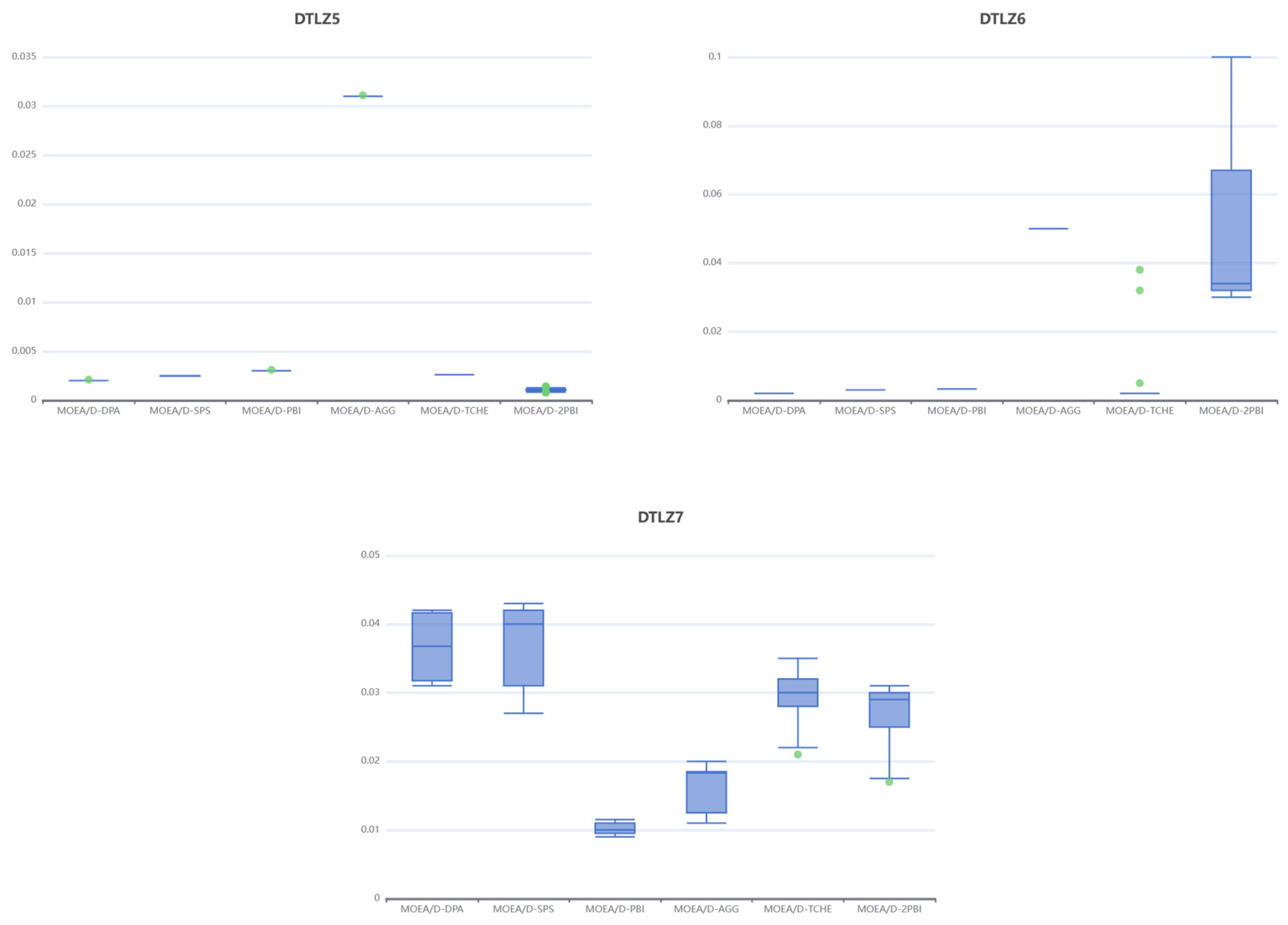
Among the seven test functions of the tri-objective problem, the DPA strategy finds the optimal IGD values on the DTLZ2, DTLZ3, DTLZ4, and DTLZ6 test problems, but underperforms on the DTLZ7 test problem. Therefore, it is concluded that the DPA tuning strategy has some performance enhancement effect on the PBI decomposition strategy on the three-objective problem and is better than similar improved algorithms.

As can be seen from the boxplots in Figure 5, the DPA strategy achieves better IGD metrics on the ZDT1, ZDT2, and ZDT4 problems, thus proving that its derived solution sets are closer to the ideal Pareto distance. It can also be seen that the IGD metrics obtained by the DPA strategy on all four test problems are more stable than those obtained by the original PBI decomposition strategy. On the ZDT3 problem, the IGD metrics obtained by both the DPA strategy and the SPS strategy are unsatisfactory.

As demonstrated by the box plots presented in Figure 6, the MOEA/D-DPA algorithm achieves better IGD metrics than the MOEA/D-PBI algorithm on the test problems except DTZL7 and is more stable. The MOEA/D-DPA and MOEA/D-SPS algorithms do not perform well on the DTLZ7 test problem, which shows that on the triple-objective problem, the DPA decomposition strategy has some solution quality improvement over the original PBI decomposition strategy, but there is still room for improvement.

4.3.3. Analysis of HV Performance Index Results

The mean, standard deviation, median, and interquartile deviation of HV on the test set ZDT for the MOEA/D-DPA, MOEA/D-SPS, MOEA/D-PBI, MOEA/D-AGG, MOEA/D-TCHE, and MOEA/D-2PBI algorithms are given in

Table 5. HV mean and standard deviation of algorithms.

	MOEA/D-DPA	MOEA/D-SPS	MOEA/D-PBI	MOEA/D-AGG	MOEA/D-TCHE	MOEA/D-2PBI
ZDT1	6.01E-1 (3.1E-3)	5.22E-1 (4.0E-2)	4.18E-1 (4.8E-2)	6.22E-1 (3.7E-2)	5.35E-1 (4.7E-2)	1.93E-1 (8.6E-2)
ZDT2	3.10E-1 (8.0E-3)	1.97E-1 (5.4E-2)	1.97E-1 (4.2E-2)	6.51E-3 (1.7E-2)	2.35E-1 (4.1E-2)	4.05E-3 (7.9E-3)
ZDT3	3.42E-1 (4.8E-2)	2.31E-2 (5.2E-2)	2.64E-1 (5.1E-2)	3.65E-1 (7.5E-2)	2.98E-1 (3.7E-2)	1.56E-1 (2.9E-2)
ZDT4	3.63E-1 (1.4E-1)	6.82E-2 (1.3E-1)	4.28E-3 (9.3E-3)	3.25E-2 (6.1E-2)	9.39E-3 (1.9E-2)	0.00E+0 (0.00E+0)
DTLZ1	7.92E-1 (9.2E-4)	7.69E-1 (5.4E-3)	7.45E-1 (4.8E-2)	7.07E-4 (3.5E-3)	2.08E-1 (2.6E-1)	1.79E-1 (2.8E-1)
DTLZ2	4.09E-1 (2.5E-3)	3.83E-1 (4.1E-3)	3.55E-1 (5.4E-3)	8.43E-8 (6.2E-7)	3.63E-1 (2.4E-3)	2.94E-1 (1.3E-2)
DTLZ3	3.78E-1 (9.1E-2)	2.70E-1 (1.6E-1)	1.08E-1 (1.4E-1)	8.63E-6 (3.2E-9)	2.69E-2 (6.4E-2)	1.99E-2 (6.2E-2)
DTLZ4	3.76E-1 (7.2E-2)	3.39E-1 (8.3E-2)	3.36E-1 (1.6E-2)	4.42E-8 (6.2E-5)	3.29E-1 (3.3E-2)	2.83E-1 (2.3E-2)
DTLZ5	8.93E-2 (8.1E-5)	8.87E-2 (3.7E-4)	8.64E-2 (2.8E-4)	3.43E-9 (2.2E-7)	8.84E-2 (2.8E-4)	8.75E-2 (1.2E-3)
DTLZ6	9.02E-2 (7.7E-5)	8.93E-2 (3.6E-4)	8.77E-2 (1.6E-4)	2.43E-4 (5.2E-9)	8.97E-2 (6.6E-3)	8.53E-2 (2.4E-2)
DTLZ7	4.03E-3 (4.5E-3)	6.56E-3 (1.1E-2)	4.56E-2 (1.4E-2)	8.67E-2 (4.3E-2)	2.185E-3 (4.8E-3)	2.22E-2 (3.0E-2)

and

Table 6. HV median and quartile of algorithms.

	MOEA/D-DPA	MOEA/D-SPS	MOEA/D-PBI	MOEA/D-AGG	MOEA/D-TCHE	MOEA/D-2PBI
ZDT1	6.03E-1 (5.2E-3)	5.28E-1 (4.4E-2)	3.43E-1 (2.7E-1)	6.34E-1 (3.1E-2)	5.42E-1 (7.6E-2)	1.85E-1 (1.2E-1)
ZDT2	3.09E-1 (1.2E-2)	1.85E-1 (9.7E-2)	8.15E-2 (1.6E-1)	3.21E-4 (5.9E-3)	2.37E-1 (6.7E-2)	0.00E+0 (4.3E-3)
ZDT3	3.52E-1 (5.0E-3)	2.06E-2 (9.6E-2)	1.96E-1 (1.2E-1)	3.75E-1 (1.1E-1)	3.02E-1 (4.0E-2)	1.55E-1 (3.4E-2)
ZDT4	3.68E-1 (2.9E-1)	6.82E-5 (1.0E-1)	6.94E-5 (2.3E-1)	3.25E-2 (6.1E-2)	9.39E-3 (1.9E-2)	0.00E+0 (0.00E+0)
DTLZ1	7.92E-1 (1.1E-3)	7.70E-1 (3.6E-3)	7.62E-1 (1.1E-2)	3.33E-14 (4.0E-1)	1.41E-2 (4.2E-1)	7.51E-1 (8.5E-3)
DTLZ2	4.10E-1 (3.2E-3)	3.84E-1 (6.3E-3)	3.56E-1 (8.1E-3)	8.43E-8 (6.2E-7)	3.64E-1 (3.4E-3)	2.94E-1 (1.7E-2)
DTLZ3	4.03E-1 (1.1E-2)	3.67E-1 (2.7E-1)	1.37E-1 (2.6E-1)	8.63E-6 (3.2E-9)	1.53E-1 (1.6E-1)	2.75E-1 (1.8E-1)
DTLZ4	3.99E-1 (6.0E-3)	3.67E-1 (1.0E-2)	3.40E-1 (1.8E-2)	4.42E-8 (6.2E-5)	3.47E-1 (7.0E-2)	2.82E-1 (2.8E-2)
DTLZ5	8.93E-2 (8.8E-5)	8.87E-2 (4.9E-4)	8.64E-2 (3.9E-4)	3.43E-9 (2.2E-7)	8.84E-2 (4.0E-4)	8.75E-2 (1.7E-3)
DTLZ6	9.02E-2 (9.9E-6)	8.98E-2 (3.0E-4)	8.76E-2 (3.2E-4)	2.43E-4 (5.2E-9)	9.14E-2 (4.5E-4)	9.36E-2 (1.5E-3)
DTLZ7	7.25E-4 (9.1E-3)	9.09E-4 (9.9E-3)	4.68E-2 (1.9E-2)	1.12E-1 (8.7E-2)	7.27E-4 (2.2E-3)	1.01E-2 (1.6E-2)

, and a blackening operation has been performed on the better data of each algorithm.

Combining the HV performance metrics of the algorithms in Table 5 and Table 6, it can be seen that the MOEA/D-DPA algorithm has better HV metrics than the original MOEA/D-PBI algorithm and outperforms the similar improved MOEA/D-SPS and MOEA/D-2PBI algorithms on all four test problems of ZDT. And the MOEA/D-DPA algorithm finds the optimal HV metric value on ZDT2 and ZDT4 problems. Therefore, it is believed that the MOEA-DPA algorithm solution improves the convergence and diversity of the solution to the bi-objective problem.

On the three-objective problem, the improved MOEA/D-DPA algorithm performs better than the original PBI strategy on all the test problems except DTLZ7 and achieves the optimal value of the five decomposition strategies. However, it performs poorly on the DTLZ7 test problem. In summary, it is concluded that the MOEA/D-DPA algorithm enhances population diversity and improves solution quality to some extent, which is consistent with the previous conclusions.

As can be seen from Figure 7, the MOEA/D-DPA algorithm significantly improves the HV metrics over the original MOEA/D-PBI algorithm on the four ZDT test problems, especially on the ZDT2 and ZDT4 test problems, where the HV metrics obtained by the MOEA/D-DPA algorithm are optimal. In general, both IGD metrics and HV metrics combine to demonstrate the convergence and diversity of the algorithms, i.e., the dynamic parameterization strategy exhibits better performance metrics than the original PBI decomposition strategy on the ZDT test problem, but on the ZDT3 test problem, the IGD metrics of the MOEA/D-DPA algorithm are slightly worse than those of the MOEA/D-PBI algorithm, but the HV metrics are better than those of the MOEA/D-PBI algorithm. This is due to the fact that although both IGD and HV metrics combine to show the performance of the algorithms, the HV metrics are more inclined to reflect the population diversity of the algorithms. Therefore, it is proven that the MOEA/D-DPA algorithm improves population diversity in discontinuous bi-objective optimization problems. In the test problems, except for ZDT4, the metrics solved by the MOEA/D-DPA algorithm have better stability. Therefore, it is concluded that the DPA strategy improves the solution performance of the algorithm to a greater extent, which is consistent with the previous conclusion.

As can be seen from the HV boxplots of the five algorithms on the DTLZ test problem in Figure 8, the MOEA/D-DPA algorithm achieves higher performance and is more stable than the MOEA/D-SPS algorithm on the triple-objective problem in most cases. However, both the MOEA/D-DPA algorithm and the MOEA/D-SPS algorithm yielded poor HV performance metrics on the DTLZ7 test problem. Overall, it is concluded that the MOEA/D-DPA algorithm has some solution quality improvement over the MOEA/D-PBI algorithm on the triple-objective problem, but there is still some room for improvement.

5. Conclusions

In order to solve the shortcomings caused by the fixed penalty parameter in the PBI decomposition strategy in the MOEA/D algorithm, this paper proposes the MOEA/D-DPA dynamic tuning algorithm. This strategy will dynamically adjust the penalty parameter according to the current iteration period, and then adaptively adjust the value of the penalty parameter according to the distribution of solutions around the current weight vector, so as to make the population better balance between convergence and diversity while improving the operational efficiency. The experimental results show that the improved dynamic tuning parameter substantially improves the solution quality of the PBI decomposition strategy with higher stability in solving bi-objective optimization problems. In solving the three-objective optimization problem, dynamic parameter tuning improves the quality of the solution of the PBI decomposition strategy to a certain extent, and there is a certain improvement in the population diversity in. However, it also brings the problem of unstable solution. Therefore, it is considered that the tuning strategy has a certain degree of performance optimization effect on the PBI decomposition strategy in multi-objective optimization problems. Tuning strategies offer significant advantages in addressing optimization problems, providing strong support for their application to real-world issues. The MOEA/D-DPA algorithm maintains similar time and space complexity to the basic MOEA/D algorithm, while also demonstrating effective scalability in parallelized and distributed environments. This increased scalability enhances the algorithm’s applicability to real-world optimization problems.

References

- Houssein, E.H.; Mahdy, M.A.; Shebl, D.; Manzoor, A.; Sarkar, R.; Mohamed, W.M. An efficient slime mould algorithm for solving multi-objective optimization problems. Expert Syst. Appl. 2022, 187, 115870. [Google Scholar] [CrossRef]
- Wang, J.; Zhou, Y.; Li, Z. Hour-ahead photovoltaic generation forecasting method based on machine learning and multi objective optimization algorithm. Appl. Energy 2022, 312, 118725. [Google Scholar] [CrossRef]
- Liu, H.; Li, Y.; Duan, Z.; Chen, C. Review on multi-objective optimization framework in wind energy forecasting techniques and applications. Energy Convers. Manag. 2020, 224, 113324. [Google Scholar] [CrossRef]
- Bai, L.; Liu, Z.; Wang, J. Novel hybrid extreme learning machine and multi-objective optimization algorithm for air pollution prediction. Appl. Math. Model. 2022, 106, 177–198. [Google Scholar] [CrossRef]
- Gautier, N.J.D.; Manzanares Filho, N.; Da Silva Ramirez, E.R. Multi-objective optimization algorithm assisted by metamodels with applications in aerodynamics problems. Appl. Soft Comput. 2022, 117, 108409. [Google Scholar] [CrossRef]
- Yang, S.; Jiang, Y. Improving the multiobjective evolutionary algorithm based on decomposition with new penalty schemes. Soft Comput. 2017, 21, 4677–4691. [Google Scholar] [CrossRef]
- Konak, A.; Coit, D.W.; Smith, A.E. Multi-objective optimization using genetic algorithms: A tutorial. Reliab. Eng. Syst. Saf. 2006, 91, 992–1007. [Google Scholar] [CrossRef]
- Zhang, Q.; Li, H. MOEA/D: A Multiobjective Evolutionary Algorithm Based on Decomposition. IEEE Trans. Evol. Comput. 2007, 11, 712–731. [Google Scholar] [CrossRef]
- Wang, M.; Heidari, A.A.; Chen, H. A multi-objective evolutionary algorithm with decomposition and the information feedback for high-dimensional medical data. Appl. Soft Comput. 2023, 136, 110102. [Google Scholar] [CrossRef]
- Cheng, F.; Chu, F.; Xu, Y.; Zhang, L. A steering-matrix-based multiobjective evolutionary algorithm for high-dimensional feature selection. IEEE Trans. Cybern. 2021, 52, 9695–9708. [Google Scholar] [CrossRef]
- Sonoda, T.; Nakata, M. Multiple classifiers-assisted evolutionary algorithm based on decomposition for high-dimensional multiobjective problems. IEEE Trans. Evol. Comput. 2022, 26, 1581–1595. [Google Scholar] [CrossRef]
- Pruvost, G.; Derbel, B.; Liefooghe, A.; Li, K.; Zhang, Q. On the combined impact of population size and sub-problem selection in MOEA/D. In Proceedings of the Evolutionary Computation in Combinatorial Optimization: 20th European Conference, EvoCOP 2020, Seville, Spain, 15–17 April 2020; Held as Part of EvoStar 2020; Proceedings 20. Springer International Publishing: Cham, Switzerland, 2020; pp. 131–147. [Google Scholar] [CrossRef]
- Wu, X.; Chen, C.; Ding, S. A modified MOEA/D algorithm for solving bi-objective multi-stage weapon-target assignment problem. IEEE Access 2021, 9, 71832–71848. [Google Scholar] [CrossRef]
- Xie, Y.; Yang, S.; Wang, D.; Qiao, J.; Yin, B. Dynamic transfer reference point-oriented MOEA/D involving local objective-space knowledge. IEEE Trans. Evol. Comput. 2022, 26, 542–554. [Google Scholar] [CrossRef]
- Liu, S.; Lin, Q.; Wong, K.C.; Coello, C.A.C.; Li, J.; Ming, Z.; Zhang, J. A self-guided reference vector strategy for many-objective optimization. IEEE Trans. Cybern. 2020, 52, 1164–1178. [Google Scholar] [CrossRef] [PubMed]
- Wang, C.; Huang, H.; Pan, H. A constrained many-objective evolutionary algorithm with learning vector quantization-based reference point adaptation. Swarm Evol. Comput. 2023, 82, 101359. [Google Scholar] [CrossRef]
- Jiao, R.; Zeng, S.; Li, C.; Ong, Y.S. Two-type weight adjustments in MOEA/D for highly constrained many-objective optimization. Inf. Sci. 2021, 578, 592–614. [Google Scholar] [CrossRef]
- Zhang, Y.; Wang, G.G.; Li, K.; Yeh, W.C.; Jian, M.; Dong, J. Enhancing MOEA/D with information feedback models for large-scale many-objective optimization. Inf. Sci. 2020, 522, 1–16. [Google Scholar] [CrossRef]
- Yang, L.; Jia, X.; Xu, R.; Cao, J. An MOEA/D-ACO Algorithm with Finite Pheromone Weights for Bi-objective TTP. In Proceedings of the Data Mining and Big Data: 6th International Conference, DMBD 2021, Guangzhou, China, 20–22 October 2021; Proceedings, Part I 6. Springer: Singapore, 2021; pp. 468–482. [Google Scholar] [CrossRef]
- Wan, X.; Lian, H.; Ding, X.; Peng, J.; Wu, Y.; Li, X. Hierarchical multiobjective dispatching strategy for the microgrid system using modified MOEA/D. Complexity 2020, 2020, 4725808. [Google Scholar] [CrossRef]
- Zhang, H.; Yue, D.; Yue, W.; Li, K.; Yin, M. MOEA/D-based probabilistic PBI approach for risk-based optimal operation of hybrid energy system with intermittent power uncertainty. IEEE Trans. Syst. Man Cybern. Syst. 2019, 51, 2080–2090. [Google Scholar] [CrossRef]
- Liu, W.; Zhang, Q.; Tsang, E.; Virginas, B. Tchebycheff approximation in Gaussian Process model composition for multi-objective expensive black box. In Proceedings of the 2008 IEEE Congress on Evolutionary Computation, Hong Kong, China, 1–6 June 2008; IEEE World Congress on Computational Intelligence. IEEE: Piscataway, NJ, USA, 2008; pp. 3060–3065. [Google Scholar] [CrossRef]
- Wang, R.; Ishibuchi, H.; Zhang, Y.; Zheng, X.; Zhang, T. On the effect of localized PBI method in MOEA/D for multi-objective optimization. In Proceedings of the 2016 IEEE Symposium Series on Computational Intelligence (SSCI), Athens, Greece, 6–9 December 2016; IEEE: Piscataway, NJ, USA, 2016; pp. 1–8. [Google Scholar]
- Sato, H. Inverted PBI in MOEA/D and its impact on the search performance on multi and many-objective optimization. In Proceedings of the 2014 Annual Conference on Genetic and Evolutionary Computation, Vancouver, BC, Canada, 12–16 July 2014; pp. 645–652. [Google Scholar] [CrossRef]
- Guo, J.; Yang, S.; Jiang, S. An adaptive penalty-based boundary intersection approach for multiobjective evolutionary algorithm based on decomposition. In Proceedings of the 2016 IEEE Congress on Evolutionary Computation (CEC), Vancouver, BC, Canada, 24–29 July 2016; IEEE: Piscataway, NJ, USA, 2016; pp. 2145–2152. [Google Scholar] [CrossRef]
- Ishibuchi, H.; Akedo, N.; Nojima, Y. Behavior of multiobjective evolutionary algorithms on many-objective knapsack problems. IEEE Trans. Evol. Comput. 2015, 19, 264–283. [Google Scholar] [CrossRef]
- Sato, Y.; Hirayama, T.; Ikami, R. Adaptive PBI for Massively Parallel MOEA/D in a Distributed Memory Environment. In Proceedings of the 2022 IEEE Congress on Evolutionary Computation (CEC), Padua, Italy, 18–23 July 2022; IEEE: Piscataway, NJ, USA, 2022; pp. 1–8. [Google Scholar] [CrossRef]
- Huang, Z.; Zhou, Y.; Luo, C.; Lin, Q. A Runtime Analysis of Typical Decomposition Approaches in MOEA/D Framework for Many-objective Optimization Problems. In Proceedings of the Thirtieth International Joint Conference on Artificial Intelligence, IJCAI, Montreal, QC, Canada, 19–27 August 2021; pp. 1682–1688. [Google Scholar] [CrossRef]
- Wang, Z.; Deng, J.; Zhang, Q.; Yang, Q. On the parameter setting of the penalty-based boundary intersection method in MOEA/D. In Proceedings of the International Conference on Evolutionary Multi-Criterion Optimization, Shenzhen, China, 28–31 March 2021; Springer International Publishing: Cham, Switzerland, 2021; pp. 413–423. [Google Scholar] [CrossRef]
- Pang, L.M.; Ishibuchi, H.; Shang, K. Use of two penalty values in multiobjective evolutionary algorithm based on decomposition. IEEE Trans. Cybern. 2022, 53, 7174–7186. [Google Scholar] [CrossRef] [PubMed]
Figure 1.
A note on the underpunishment of weight vectors using , , = 1.0 in PBI.
Figure 2.
A note on the underpunishment of weight vectors using , , = 5.00 in PBI.
Figure 3.
Results of five algorithms in ZDT problem.
Figure 4.
Results of algorithms in the DTLZ problem.
Figure 5.
Box plots of IGD of algorithms on ZDT test suites.
Figure 6.
Box plots of the IGD of algorithms on DTLZ test suites.
Figure 7.
Box plots of HV of algorithms on ZDT test suites.
Figure 8.
Box plots of the HV of algorithms on DTLZ test suites.