
The Impact of GCP Chip Distribution on Kompsat-3A RPC Bias Compensation

1
Interdisciplinary Major of Ocean Renewable Energy Engineering, Korea Maritime and Ocean University, Busan 49112, Republic of Korea
2
Department of Civil Engineering, Seoul National University of Science and Technology, Seoul 01811, Republic of Korea
3
Department of Civil Engineering, Korea Maritime and Ocean University, Busan 49112, Republic of Korea
*
Author to whom correspondence should be addressed.
Appl. Sci. 2024, 14(8), 3482; https://doi.org/10.3390/app14083482
Submission received: 5 March 2024
/
Revised: 10 April 2024
/
Accepted: 19 April 2024
/
Published: 20 April 2024
(This article belongs to the Special Issue Selected Papers from the 12th International Multi-Conference on Engineering and Technology Innovation (IMETI 2023))
Abstract
:The vast potential of high-resolution satellite images, including Kompsat-3A, has been demonstrated across diverse applications, such as mapping and disaster monitoring. However, these images can only be utilized as reliable GIS (geographic information system) data when they possess precise geographical information. To achieve this, sensor model information, represented by RPCs (rational polynomial coefficients), requires bias compensation through GCPs (ground control points). Though having a substantial number of well-distributed GCPs across satellite images is ideal, the acquisition process is often restricted due to cost and inaccessibility. The uniform distribution of GCP chips is not guaranteed, necessitating an investigation into the impact of GCP distribution on the bias compensation process, which is the focus of this study. Experiments were meticulously conducted using Kompsat-3A data using dense GCP information. The dense GCP information was automatically generated from aerial orthoimages through a three-step process. Firstly, the GCP chips were extracted from the aerial images, focusing on feature points. Secondly, these chips were projected onto the target Kompsat-3A data to align them accurately. Lastly, precise satellite image coordinates of the chips were obtained through image matching between the chips and the target Kompsat-3A image. The dense GCPs enabled detailed bias analysis that exhibited skewness in most Kompsat-3A data. This necessitates the implementation of an affine model for proper bias compensation over the entire image space. Next, the study delved into the influence of GCP distribution on RPC bias compensation. To this end, each target satellite image space was divided into nine zones, with the dense GCPs assigned accordingly. The accuracy of bias compensation was analyzed across nine experimental cases, ranging from GCPs occupying only one zone to GCPs covering all nine zones. It was observed that GCPs covering at least four or five zones should be utilized for reliable RPC bias compensation of Kompsat-3A, especially when aiming for a high level of accuracy with an RMSE of one pixel. Finally, it was concluded that GCPs covering three zones yielded satisfactory results as a minimum GCP requirement, but this was contingent upon their distribution not following a straight zone pattern.
1. Introduction
The vast potential of high-resolution satellite images has been demonstrated across diverse applications, including mapping and disaster monitoring. However, these images can only be utilized as reliable GIS (geographic information system) data when they possess precise geographical information. Geometric processing requires the sensor model information supplied in RPCs (rational polynomial coefficients) [1]. However, the sensor model information is biased due to the limited accuracy of satellite orbits and attitudes.
Post-processing is required for bias compensation using reliable ground control points known as GCPs (ground control points) [2]. Therefore, numerous research efforts have focused on the generic bias compensation of RPCs using GCPs [2,3,4,5,6]. They emphasized the importance of GCPs for bias compensation. Additionally, many studies have tested bias compensation models for achievable accuracy in targeted high-resolution satellite images, such as IKONOS [5], QuickBird [7], Kompsat-2 [8], GeoEye-1 [9], WorldView-1/2 [10], TH-1 [11], and Ziyuan-3 [12].
While having a substantial number of well-distributed GCPs across satellite images is ideal, the acquisition process is often restricted due to cost and inaccessibility [12,13]. Consequently, GCP chips have recently been generated from an existing database and employed for bias compensation [14]. Nevertheless, the uniform distribution of GCP chips is not guaranteed, necessitating an investigation into the impact of GCP distribution on the bias compensation process.
Several studies have examined the distribution of GCPs for geometrically correcting geospatial images [12,15,16,17]. One study compared various sensor models using different numbers of GCPs [12], suggesting that fixing four GCPs in the corners of the target image was optimal. Another investigation focused on the densification effect of GCPs in aerial image geometric processing [15], concluding that poor locations and distributions increased geometric errors, recommending three GCPs for cost-effective processing. In a separate study [16], the bias compensation of IKONOS RPCs for different GCP cases was explored, advocating that four GCPs suffice, saving time and costs. Moreover, a study on stereo WorldView-2 [17] highlighted that GCP distribution outweighs the number of GCPs in geometric processing. While prior studies have emphasized the importance of GCP distribution [11,17], their recommendations vary due to differences in satellite characteristics regarding orbit and attitude information stability and reliability.
This study focuses on Kompsat-3A, providing a PAN (panchromatic) resolution of 0.55 m, an MS (multi-spectral) resolution of 2.20 m, and a TIR (thermal infrared) resolution at 5.5 m [18]. The specified positional accuracy for Kompsat-3A is 70 m (CE90), although its actual accuracy surpasses this specification [16]. Kompsat-3A also requires post-processing for RPC bias compensation using GCPs. Previous studies have indicated that GCPs need to be used efficiently in terms of time and cost [13]. Consequently, we investigated the impact of GCP distribution on Kompsat-3A. While abundant GCPs are needed across the entire image space, gathering this information is expensive. Therefore, we implemented an automated procedure to extract GCP image chips with ground coordinates from precise aerial orthoimages. Kompsat-3A image coordinates for these chips were determined using robust image-matching techniques. Subsequently, experiments were conducted based on diverse GCP distribution scenarios using this dense GCP information. Lastly, the study continued to determine the minimum GCP distribution requirement.
2. Methodology
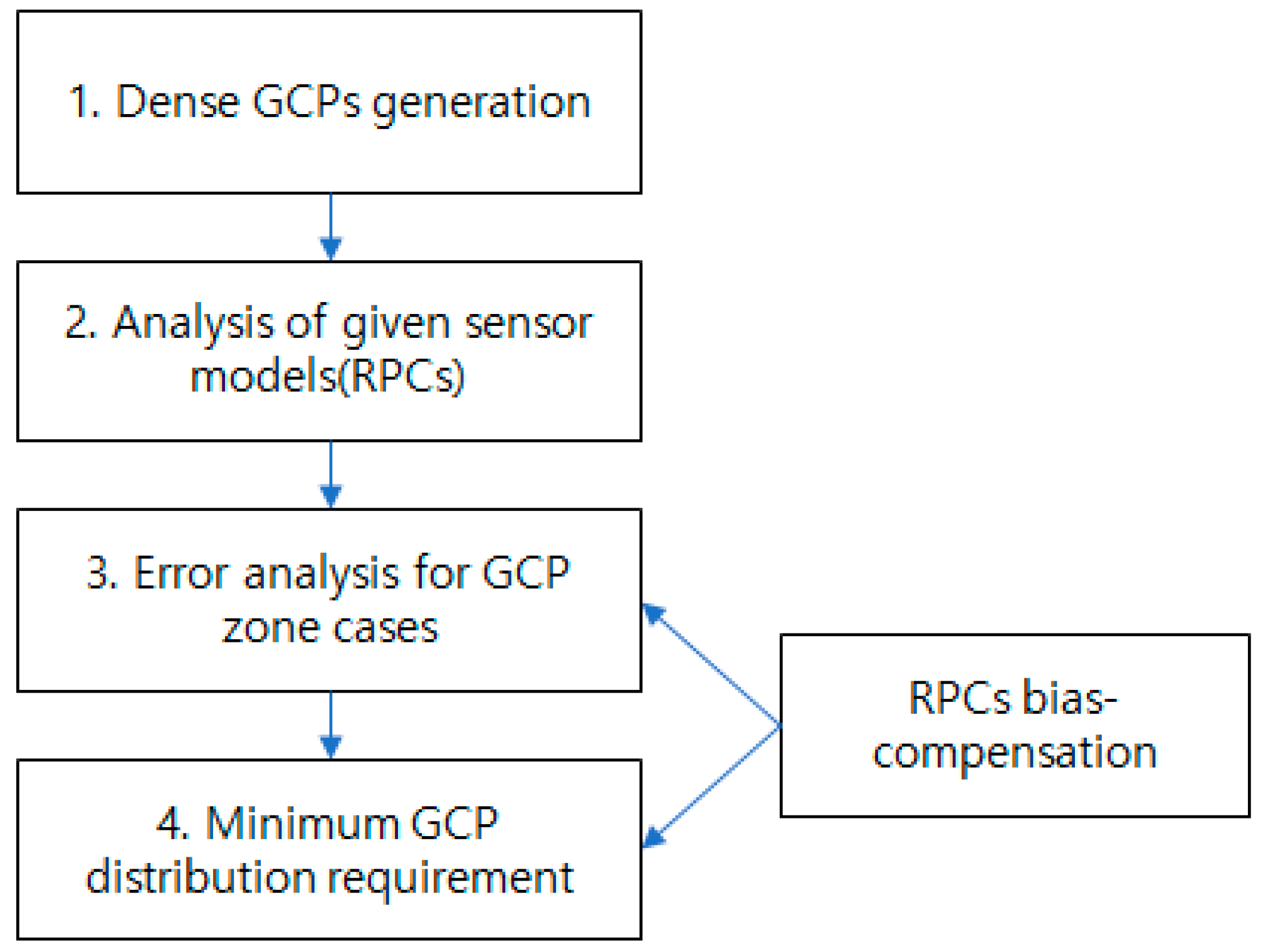
The study’s flowchart is depicted in Figure 1. Its primary aim is to analyze error patterns in Kompsat-3A data across experimental cases based on varying GCP conditions. This investigation necessitates a substantial quantity of GCPs, making the dense generation of GCPs the initial step. This process employs automation based on aerial image chips and robust image-matching techniques to generate GCPs. The study involves scrutinizing the geometric errors across the entire image area of Kompsat-3A using the abundance of generated GCPs. Following this, GCPs are allocated zone numbers based on their distribution across the target Kompsat-3A images. Experimental cases are then established to examine the impact of the number of GCP zones on sensor modeling errors. Finally, the study aims to determine the minimum GCP distribution requirement for achieving high-precision geometric correction at the one-pixel level.
Compared to other studies [12,15,16,19], our methodology has innovative aspects in that the Kompsat-3A local geometric error pattern is investigated within the image space. This is possible because dense but accurate GCPs are automatically generated using image matching with the outlier removal technique. Firstly, this study shows that Kompst-3A has large geometric error changes within the local image space. Note that most research has focused on overall georeferencing error analysis, not a local error change pattern within the image space. Secondly, this study tested the local GCP distribution cases from local error pattern analysis to avoid hazardous GCP distribution.
2.1. Sensor Model (RPCs)
The sensor model of an Earth-observing satellite defines the relationship between satellite image coordinates and ground coordinates for use in GIS data. Since IKONOS’ launch in 1999, the RFM (rational function model) has remained the most popular equation for sensor modeling. The RFM equation, provided as Equation (1), calculates satellite image coordinates based on the given ground coordinates [1]. This equation requires a total of 80 coefficients, distributed as 20 coefficients each for , and , collectively known as RPCs. These RPCs encompass the modeling of focal length, lens distortions, acquisition angles, orbit errors, and target topographic reliefs as polynomial coefficients
with
where represent ground coordinates, such as latitude, longitude, and ellipsoidal height. denote the corresponding satellite image coordinates, such as row and column. represent the normalized ground coordinates, respectively. and denote the offset and scale factors used to normalize latitude, longitude, height, column, and row.
2.2. RPC Bias Compensation
The RPCs provided by a satellite data vendor or supplier are often erroneous, resulting in computed image coordinates that have biases. This discrepancy arises due to measurement uncertainties from onboard global navigation satellite system (GNSS) receivers, star trackers, and gyroscopes [8]. The error sizes and patterns vary depending on the systems in use. Therefore, the most widely adopted method to compensate for these errors or biases is to employ an affine transform, as illustrated in Equation (2) [2]. According to this equation, the bias-compensated coordinates can be computed using transformation parameters that need to be estimated using GCPs
where are for an affine transformation that models shift, drift, and scale to the angular affinity that exists in satellite images.
2.3. Dense GCP Acquisition
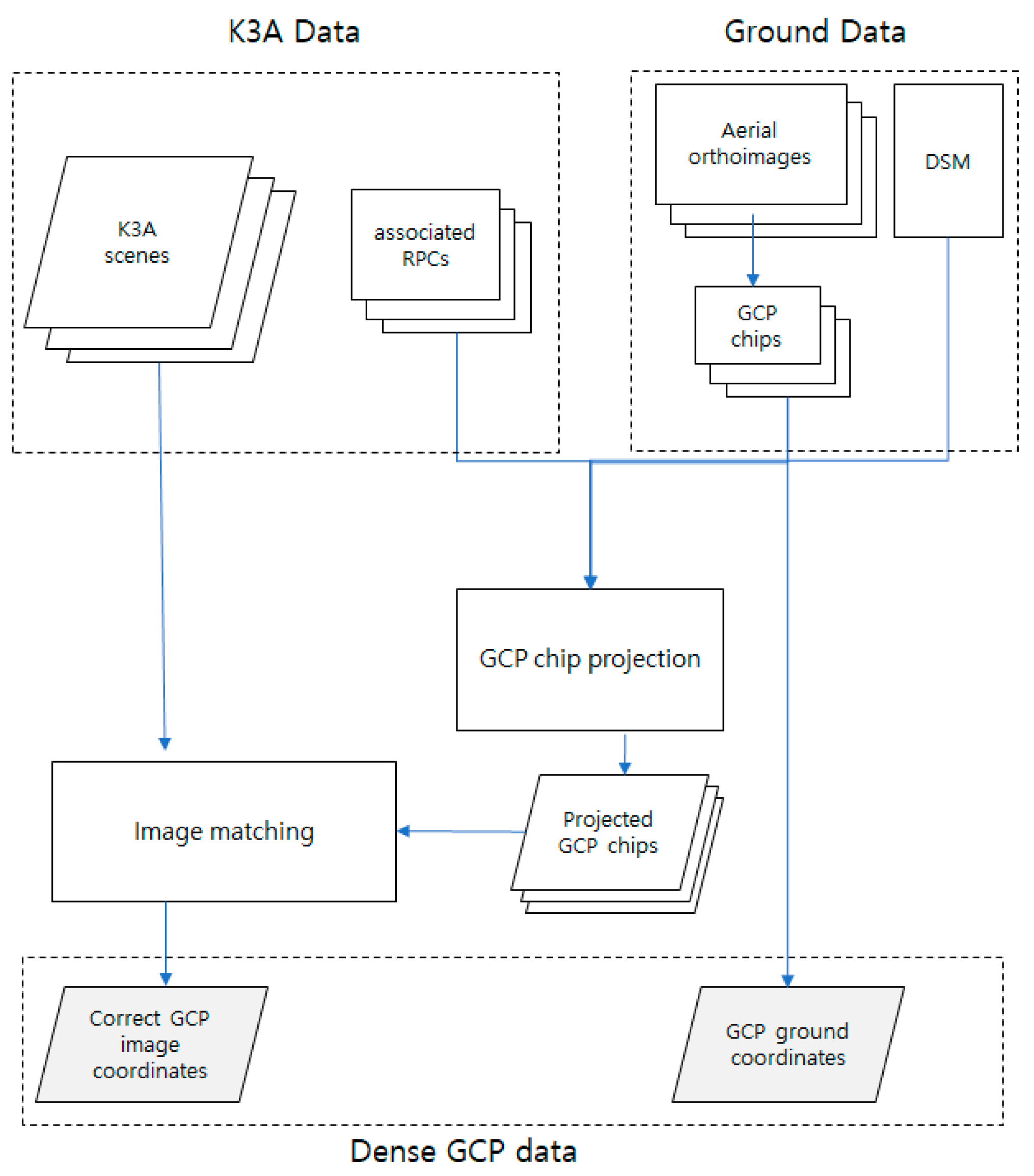
The error analysis of Kompsat-3A images demands extensive GCP information across the entire image space. GCP information comprises 3D ground coordinates such as latitude, longitude, and ellipsoidal height, along with corresponding 2D satellite image coordinates. Traditionally, acquiring GCPs involves a manual approach by a human operator, which is time consuming and labor intensive. To address this limitation, we employed an automated procedure, as outlined in Figure 2. Numerous GCP image chips were automatically extracted from aerial orthoimages and linked with a DSM (digital surface model) for elevation data, ensuring accurate 3D ground coordinate information.
The subsequent step involved the automated retrieval of corresponding Kompsat-3A image coordinates. This was achieved using robust image-matching techniques between the GCP image chips and the targeted Kompsat-3A images. Before image matching, the GCP chips were projected onto each Kompsat-3A image to calculate the associated image coordinates, such as in Equation (1). However, due to inherent errors in the associated RPC information, the computed image coordinates were biased. Hence, the image-matching process aimed to determine the correct image coordinates of the chips, represented as in Equation (2). Finally, a comparison between the computed image coordinates and the correct image coordinates was conducted to analyze locational errors. This study utilized a hybrid method of NCC (normalized cross-correlation) and RECC (relative edge cross-correlation) for image matching [13].
2.4. GCP Distribution Design
The mentioned RPCs contain inherent errors, necessitating post-processing to enhance the information’s accuracy. This process relies on accurate and well-distributed GCPs across the entire image space, as illustrated in Figure 3a. Biased distributions, as depicted in Figure 3b, are generally less desirable. However, acquiring this information is costly, emphasizing the need for the minimum and efficient utilization of GCPs. Furthermore, information acquisition becomes more limited when the target area is situated in inaccessible regions, such as North Korea.
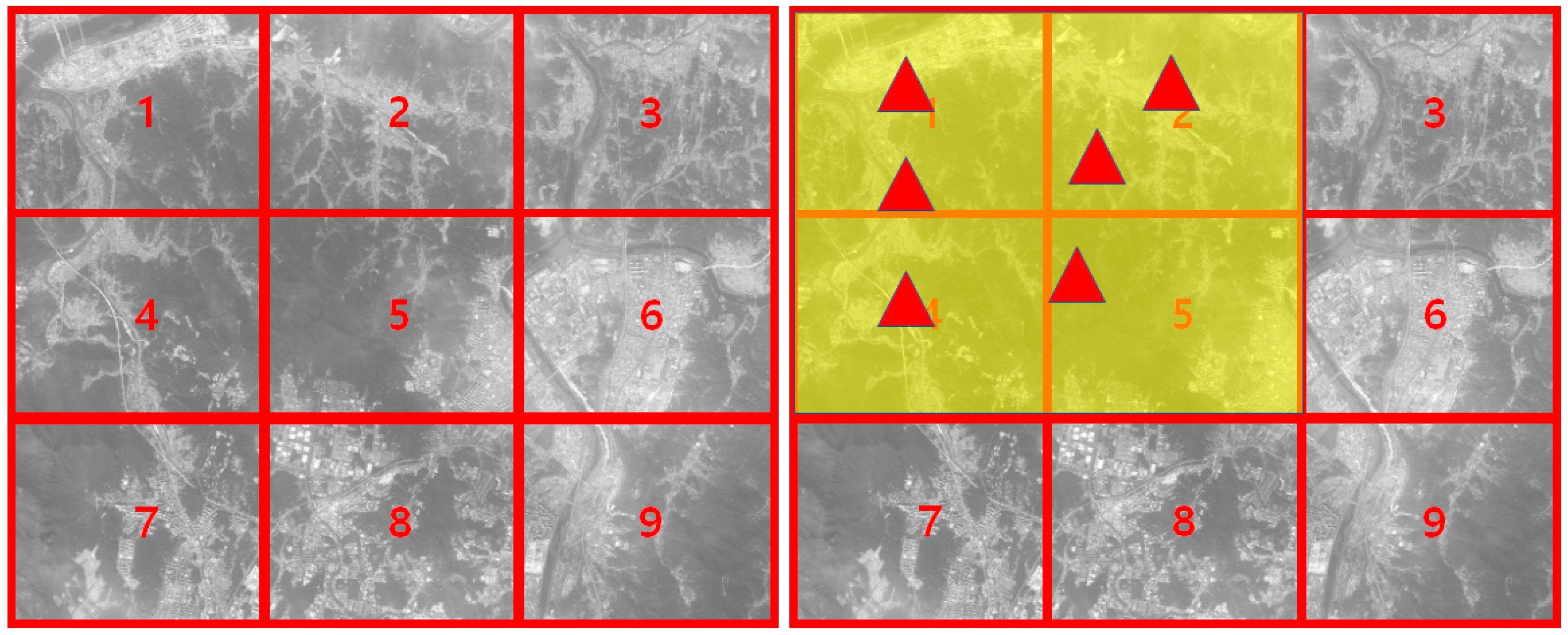
Hence, we partitioned the image space into 9 zones, as illustrated in Figure 4. This division resulted in a total of 511 experimental cases, encompassing various distributions: 9 single-zone distributions, 126 cases of five-zone distributions (9C5), 84 cases of three-zone distributions (9C3), and 1 nine-zone distribution, among others. We proceeded to analyze the impact of these derived GCP distribution scenarios.
3. Experimental Results
3.1. Data
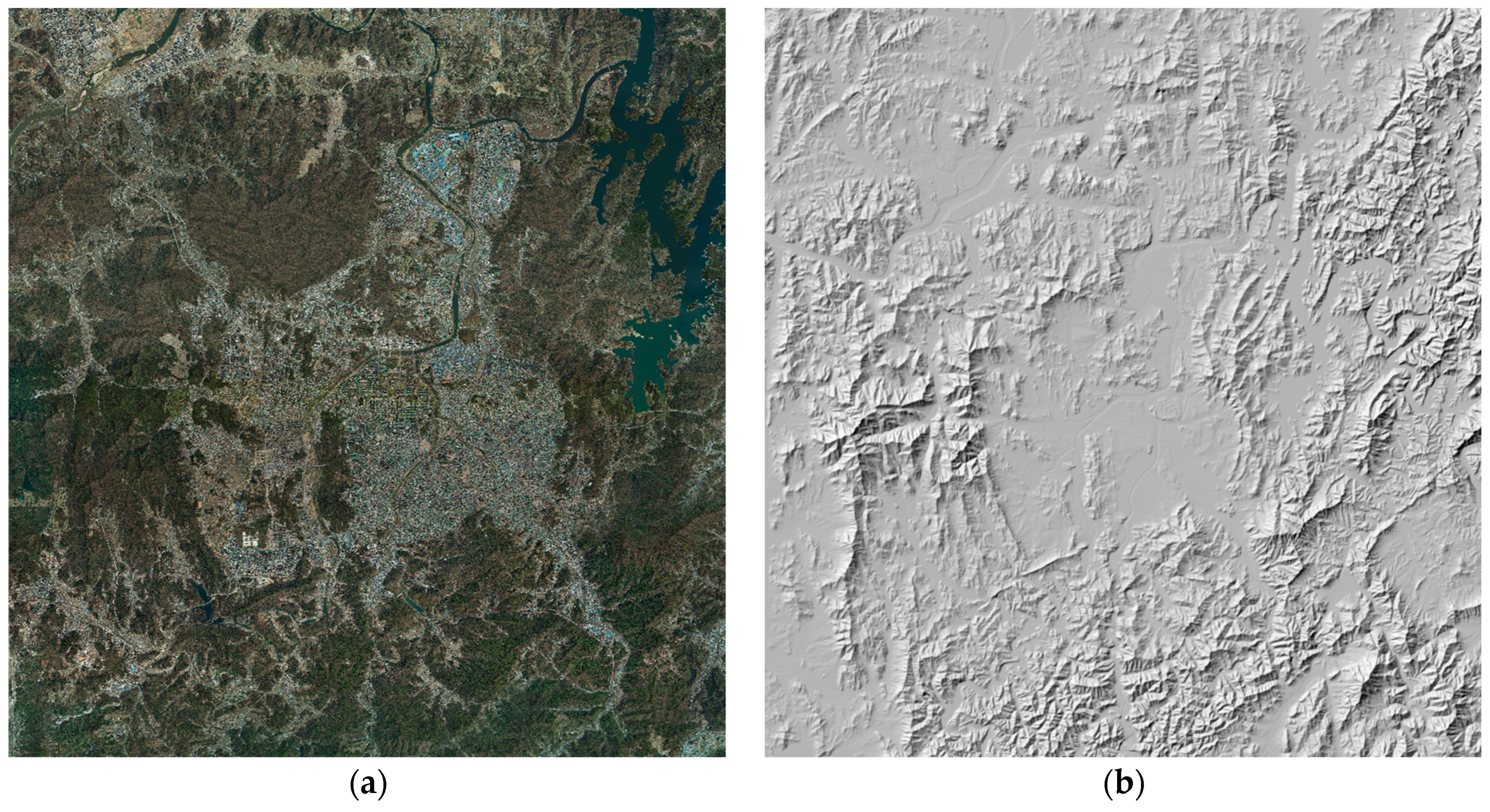
Experiments were conducted using eight Kompsat-3A images covering South Korea, with the detailed specifications presented in Table 1 and described in the thumbnails provided in Figure 5. These images were acquired between 18 October 2015 and 25 November 2020, with each image spanning approximately 16 km × 16 km at a spatial resolution of 0.6~0.7 m. The target area was carefully chosen to encompass both urban and mountainous regions, considering their potential for ground control and check points. It is important to note that the abundance of geographical features in urban and nearby areas provides robust ground control information. Table 2 outlines the specifications of the aerial orthoimages and DSM utilized for ground control and check point information. A total of 132 aerial orthoimages, each with a spatial resolution of 25 cm, were used in conjunction with 5 m DSM data. Figure 6 displays the mosaic created from the aerial orthoimages and DSM. The aerial orthoimages were generated according to the regulations of the Korean government for orthoimage generation. The positional accuracy of the orthoimages is within 25 cm in RMSE (root mean square error). The aerial orthoimages were mosaiced and divided into coverage of 1 minute and 30 s (about 2.7 km × 2.7 km).
3.2. GCP Chip Generation
The GCP information should comprise 3D ground coordinates along with their corresponding target image coordinates. The extraction of 3D ground coordinates was performed using the aerial orthoimage and its associated DSM. Key points, uniformly distributed across the aerial orthoimages, were extracted using the Harris corner point operator [20] at specified intervals, as illustrated in Figure 7. Image chips measuring 1027 × 1027 pixels around these key points were extracted and stored as GCP chips along with their ground coordinates.
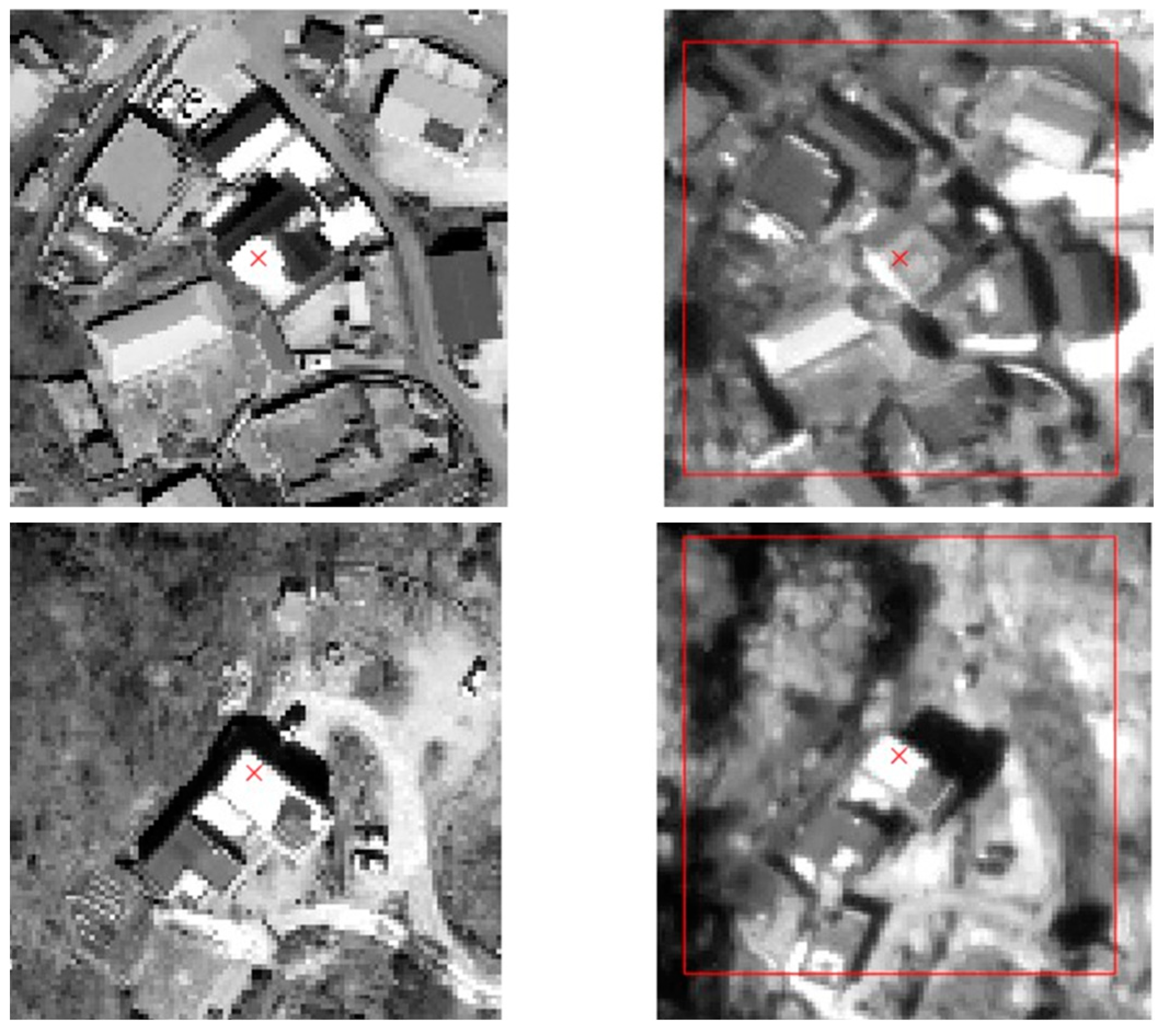
Subsequently, acquiring the corresponding Kompsat-3A image coordinates became necessary. These coordinates can be obtained through an image-matching technique applied between the GCP chips and the targeted Kompsat-3A images. However, performing image matching with heterogeneous data presents a challenge. Therefore, we implemented a procedure involving two distinct steps. The first step involves the image projection of a GCP chip onto the targeted Kompsat-3A image. This step aligns the two datasets by minimizing geometric disparities between them. An example of this projection is depicted in Figure 8. It is important to note that the projected images adopt the Kompsat-3A satellite image coordinate systems. Although the projected aerial images closely resemble the target image, the center coordinates (indicated as ‘x’) still exhibit shifts due to biases in the sensor model information.
In Figure 9, the left-most image represents an extracted aerial chip in the ground coordinate system, while the remaining images depict projections of the target Kompsat-3A images. These projections utilize the RPCs of each target image, aligning the projected images with the target Kompsat-3A images. Consequently, each projected image differs from the others owing to the varying acquisition angles of the target Kompsat-3A images.
The second step in acquiring Kompsat-3A image coordinates involves image matching. In this study, we employed both area-matching (Figure 10) and edge-matching techniques (Figure 11) to address the substantial spectral differences between the aerial GCP chip and the targeted Kompsat-3A image [13]. These differences arise from variations in sensors, acquisition dates, weather conditions, and acquisition angles. Furthermore, the matching results should account for outlier matching points. Therefore, we implemented an outlier removal process based on data snooping [21] to detect and eliminate outliers, ensuring reliable control point information.
3.3. Kompsat-3A Error Pattern Analysis
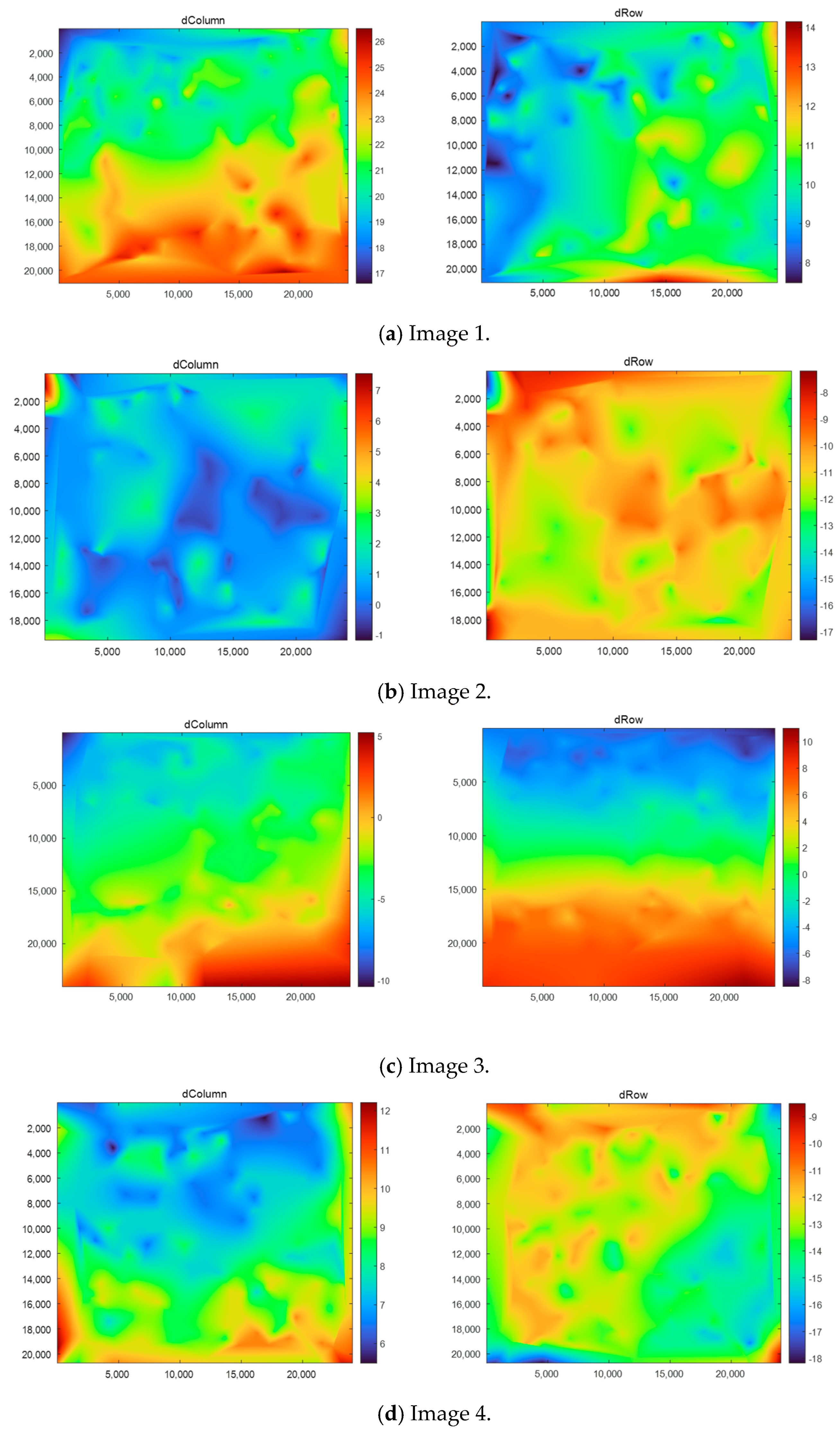
Utilizing the dense GCP information obtained earlier, we performed an error pattern analysis of the provided RPCs across the entire image. At each GCP location, we compared the RPC-estimated target image coordinates to the correct image coordinates , derived from robust image matching. Subsequently, we depicted coordinate errors along the column (sample) and row (line) in different colors, as shown in Figure 13.
All tested images exhibited distinct error patterns, with no uniform error distribution across each image. The errors ranged from −28 to 31 pixels, corresponding to approximately 18~20 m, considering the ground sample distance (GSD) of the Kompsat-3A data. Notably, Images 1, 3, and 8 displayed discernible patterns where the error distinctly increased or decreased with the progression of the image line. In the case of Image 3, these differences reached up to 18 pixels, though Image 2 demonstrated a relatively uniform error distribution across its area compared to the other images.
Based on this analysis, we concluded that the bias across the entire Kompsat-3A image area is non-uniform, with significant error fluctuations along the image line direction. This analysis indicates that GCPs with good distribution along the image line are required.
3.4. Impact of the Distribution
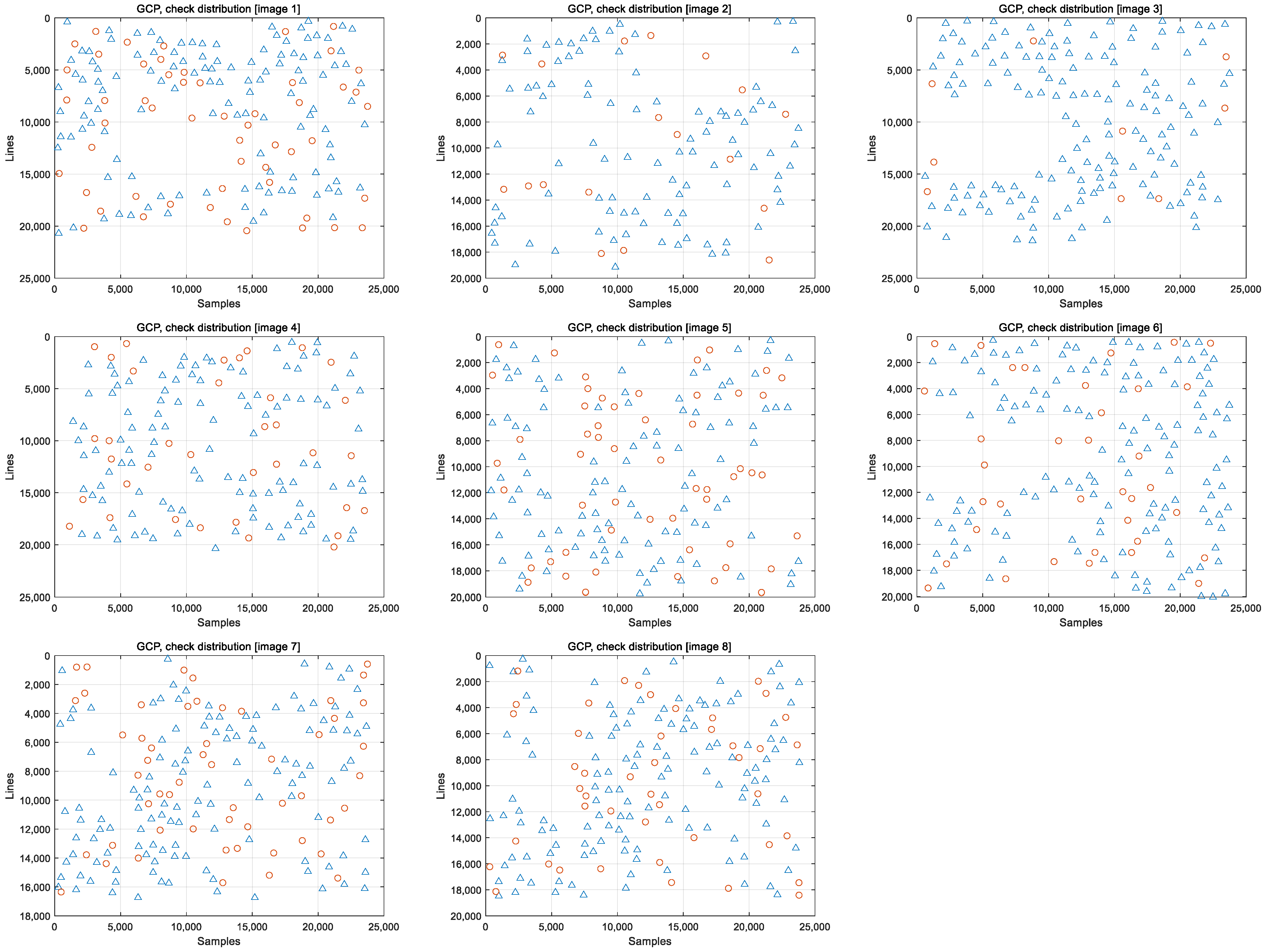
Subsequently, we aimed to assess the attainable accuracy while minimizing the number of GCPs needed. To achieve this, we subdivided the GCPs depicted in Figure 7 into GCPs and check points, as depicted in Figure 14. Note that the check points were also distributed across the entire image. Following this, we assigned zone numbers from one to nine to the remaining GCPs, as illustrated in Figure 4.
Utilizing the GCPs with assigned zone numbers, we conducted an analysis of achievable accuracy using RPC bias compensation by varying the number of GCP zones. Figure 15 illustrates the RMSE error for each Kompsat-3A image. As the number of zones increases, the accuracy improves. However, accuracy stabilizes from three or four zones, indicating the attainment of accuracy at the one-pixel level.
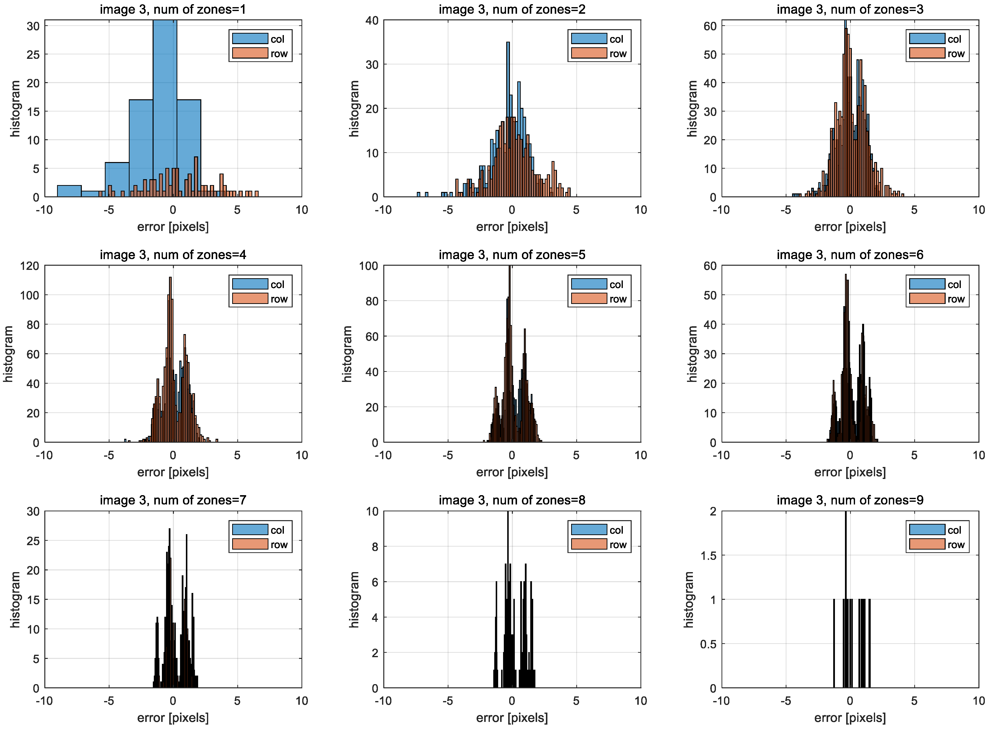
For a more detailed error analysis, an error histogram is provided for Image 3 as an example in Figure 16. The error spans from −5 pixels to +5 pixels in the case of three zones, indicating a considerable range. To achieve higher accuracy, such as within ±2 pixels, a minimum of five zones is necessary for this scenario.
3.5. Minimum Distribution Requirement
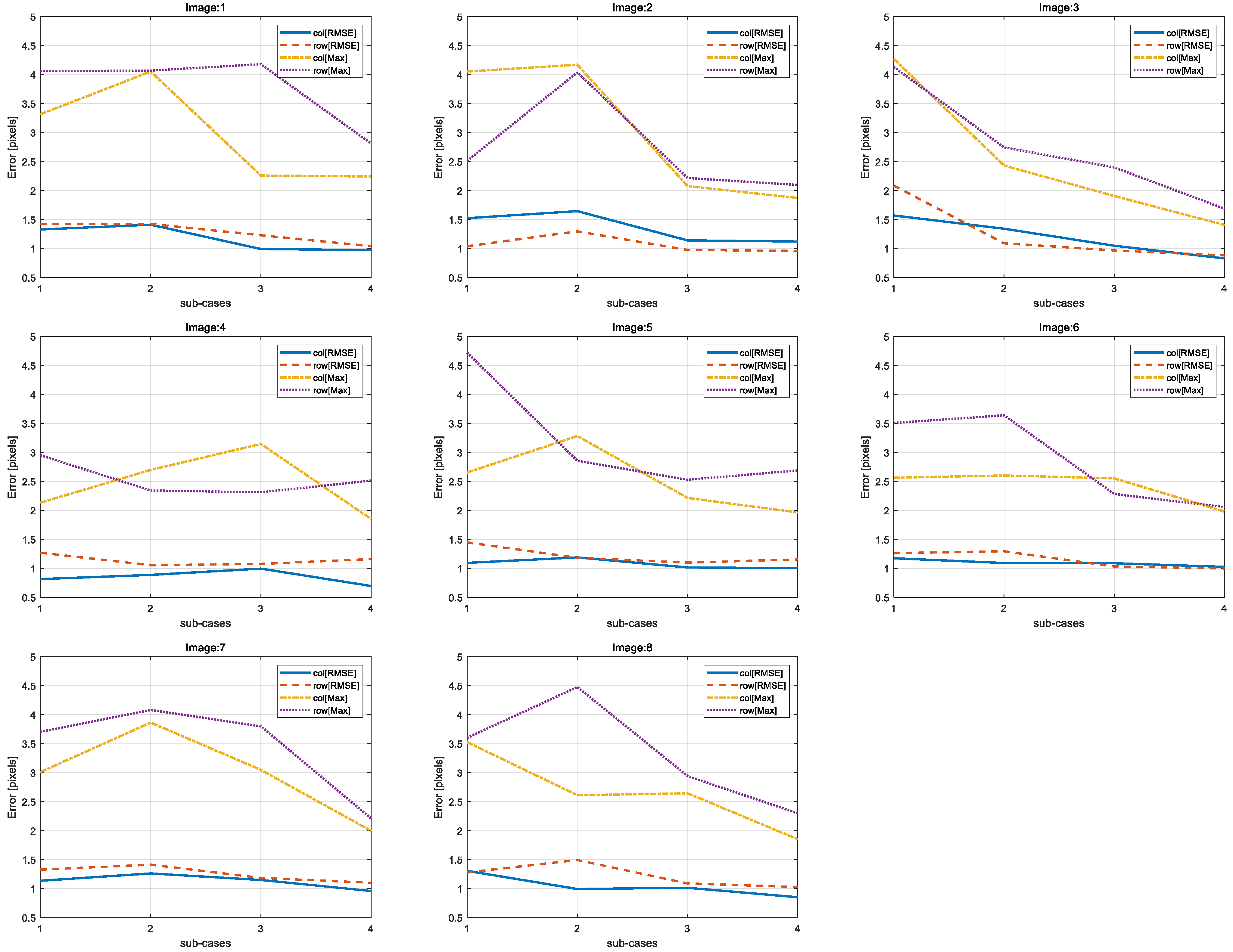
We further subdivided the three-zone cases into four sub-cases, as illustrated in Figure 17. Sub-cases 1 and 2 are column-direction and row-direction distributions, respectively. As indicated by the earlier error analysis revealing significant error changes along the image line direction (as demonstrated in Figure 13), we can expect that sub-case 1 would result in the worst accuracy. Sub-cases 2, 3, and 4 aim to encompass at least one zone along the image line direction
- Sub-case 1: 1 2 3; 4 5 6; 7 8 9
- Sub-case 2: 1 4 7; 2 5 8; 3 6 9
- Sub-case 3: 1 5 7; 2 6 8; 2 4 8; 3 5 9
- Sub-case 4: 1 6 7; 3 4 9
Figure 18 illustrates the errors observed in the proposed sub-cases. Sub-case 4 demonstrates the most favorable outcome, followed closely by sub-case 3 regarding maximum error. The error range within sub-case 4 remains within ±3 pixels (equivalent to 1 pixel in RMSE) across the entire dataset. In contrast, sub-case 1 exhibits errors ranging from 1 to 1.5 pixels, yet recording a maximum error of up to 5 pixels (observed in Image 5). As a result, we concluded that achieving accurate RPCs-bias compensation for Kompsat-3A necessitates GCP information covering at least three zones along the image line direction. Additionally, it is advisable to avoid a linear zone distribution, such as along the sample or line direction (horizontal or vertical).
4. Discussion
Detailed error pattern analysis in satellite image bias modeling necessitates abundant and well-distributed GCPs across the target image. Manual acquisition of numerous GCPs is impractical due to time and cost constraints, as highlighted in previous studies emphasizing the need for efficiency in GCP acquisition. Consequently, most prior research relied on a limited number of GCPs, resulting in sparse data. An automated process becomes pivotal to overcoming this acquisition limitation. This process involves extracting GCP chips from aerial orthoimages and determining image coordinates using robust image-matching techniques, yielding satisfactory outcomes in this study. Robust image matching allowed for the generation of a substantial amount of GCP information up to 100–200 points per tested Kompsat-3A image space. Obtaining dense GCPs over geographically uniform areas might prove challenging such that test images over the urban area were selected in the study.
An added advantage of dense GCP information lies in their categorization into control and check points. Check points serve solely in independent error checks, not for bias modeling, but this division is limited if the GCP count is insufficient. The biases observed in the tested Kompsat-3A data ranged from −28 to 31 pixels, corresponding to approximately 18~20 m, highlighting the necessity for improvement in large-scale mapping and GIS analysis. Additionally, dense GCPs facilitated the graphical plotting of skewed error changes across the tested Kompsat-3A data. While each dataset exhibited distinct bias patterns, noticeable fluctuations in bias along the image line were evident. This non-uniform bias underscores the significance of well-distributed GCPs, aligning with insights from prior studies.
In the error analysis across diverse GCP zone cases, maximum errors reached 10 pixels for the single zone case, while errors were confined within 3 pixels for cases involving four or five zones. The three-zone case mostly yielded accuracy similar to that of the four- and five-zone cases in RMSE, yet occasional maximum errors of up to 4.5 pixels were observed. Hence, it is recommended to utilize GCPs covering at least four or five zones. In scenarios with limited GCP acquisition, such as three zones, it is advisable to avoid a straight-line zone distribution.
It is expected that more and more high-resolution satellite images including constellation satellites will be used in the fields of remote sensing and geospatial analysis. The experimental results put an emphasis on bias pattern analysis before they decide on the efficient and economic geometric processing approach for the satellite images. In addition, future research should include the exploration of alternative methods or strategies for bias compensation in scenarios where dense GCP information is not feasible or available.
5. Conclusions
The automatic derivation of dense GCP information from aerial orthoimages facilitated a detailed error pattern analysis of Kompsat-3A data. During bias analysis, most Kompsat-3A data exhibited geometric skewness, necessitating the implementation of an affine model for accurate bias compensation. The dense GCPs were categorized based on their respective zones within the Kompsat-3A image space. Subsequent error analysis was conducted for various experimental cases, ranging from GCPs occupying only one zone to those covering all nine zones. As the number of zones increased, the errors in bias modeling decreased, reaching a stabilization point observed in the cases involving three zones. These empirical findings lead to the conclusion that for reliable RPC bias compensation, especially when aiming for high accuracy with an RMSE of one pixel, GCPs covering at least four or five zones should be utilized. Notably, it was observed that GCPs covering three zones yielded satisfactory results as a minimum requirement. However, their effectiveness was contingent upon their distribution, avoiding a straightforward zoning pattern.
Author Contributions
Conceptualization, J.O. and C.L.; methodology, J.O. and C.L.; software, H.J., J.O. and C.L.; validation, H.J., J.O. and C.L.; formal analysis, J.O. and C.L.; investigation, H.J., J.O. and C.L.; resources, J.O. and C.L.; data curation, H.J., J.O. and C.L.; writing—original draft preparation, H.J.; writing—review and editing, J.O. and C.L.; visualization, H.J., J.O. and C.L.; supervision, C.L.; project administration, J.O.; funding acquisition, J.O. All authors have read and agreed to the published version of the manuscript.
Funding
This study was supported by the National Research Foundation of Korea, grant number 2019R1I1A3A01062109, and the Korea Aerospace Research Institute.
Institutional Review Board Statement
Not applicable.
Informed Consent Statement
Not applicable.
Data Availability Statement
Restrictions apply to the availability of these data. Data were obtained from [Korea Aerospace and Research Institute] and are available with the permission of [Korea Aero-space and Research Institute].
Conflicts of Interest
The authors declare no conflict of interest.
References
- Fraser, C.S.; Dial, G.; Grodecki, J. Sensor orientation via RPCs. ISPRS J. Photogram. Rem. Sens 2006, 60, 182–194. [Google Scholar] [CrossRef]
- Fraser, C.S.; Hanley, H.B. Bias-compensated RPCs for sensor orientation of high-resolution satellite imagery. Photogram. Eng. Rem. Sens 2005, 71, 909–915. [Google Scholar] [CrossRef]
- Teo, T.A. Bias compensation in a rigorous sensor model and rational function model for high-resolution satellite images. Photogram. Eng. Rem. Sens 2011, 77, 1211–1220. [Google Scholar] [CrossRef]
- Topan, H. First experience with figure condition analysis aided bias compensated rational function model for georeferencing of high resolution satellite images. J. Indian Soc. Rem. Sens 2013, 41, 807–818. [Google Scholar] [CrossRef]
- Wang, J.; Di, K.C.; Li, R. Evaluation and improvement of geopositioning accuracy of IKONOS stereo imagery. J. Surv. Eng. (ASCE) 2005, 131, 35–42. [Google Scholar] [CrossRef]
- Xiong, Z.; Zhang, Y. A generic method for RPC refinement using ground control information. Photogram. Eng. Rem. Sens 2009, 75, 1083–1092. [Google Scholar] [CrossRef]
- Hong, Z.H.; Tong, X.H.; Liu, S.J.; Chen, P.; Xie, H.; Jin, Y.M. A comparison of the performance of bias-corrected RSMs and RFMs for the geo-positioning of high resolution satellite stereo imagery. Rem. Sens 2015, 7, 16815–16830. [Google Scholar] [CrossRef]
- Jeong, J.; Kim, T. Comparison of positioning accuracy of a rigorous sensor model and two rational function models for weak stereo geometry. ISPRS J. Photogram. Rem. Sens 2015, 108, 172–182. [Google Scholar] [CrossRef]
- Aguilar, M.A.; Aguilar, F.J.; Saldana, M.D.; Fernandez, I. Geopositioning accuracy assessment of GeoEye-1 panchromatic and multispectral imagery. Photogram. Eng. Rem. Sens 2012, 78, 247–257. [Google Scholar] [CrossRef]
- Alkan, M.; Buyuksalih, G.; Sefercik, U.G.; Jacobsen, K. Geometric accuracy and information content of WorldView-1 images. Opt. Eng. 2013, 52, 026201. [Google Scholar] [CrossRef]
- Dong, Y.; Lei, R.; Fan, D.; Gu, L.; Ji, S. A novel RPC bias model for improving the positional accuracy of satellite images. ISPRS Ann. Photogramm. Remote Sens. Spat. Inf. Sci. 2020, 2, 35–41. [Google Scholar] [CrossRef]
- Shen, X.; Liu, B.; Li, Q.Q. Correcting bias in the rational polynomial coefficients of satellite imagery using thin-plate smoothing splines. ISPRS J. Photogram. Remote Sens. 2017, 125, 125–131. [Google Scholar] [CrossRef]
- Mezouar, O.; Meskine, F.; Boukerch, I. Automatic satellite images orthorectification using K–means based cascaded meta-heuristic algorithm. Photogram. Eng. Rem. Sens 2023, 89, 291–299. [Google Scholar] [CrossRef]
- Oh, J.H.; Seo, D.C.; Lee, C.N.; Seong, S.K.; Choi, J.H. Automated RPCs bias compensation of KOMPSAT imagery using aerial GCPs chips in Korea. IEEE Access 2022, 10, 118465–118474. [Google Scholar] [CrossRef]
- Babiker, M.; Akhadir, S. The effect of densification and distribution of control points in the accuracy of geometric correction. IJSSRET 2016, 2, 65–70. [Google Scholar]
- Tawfeik, M.; Elhifnawy, H.; Hamza, E.; Shawky, A.; Ragab, A. Enhancement of RPC positioning accuracy using affine transformation with different number of ground control points. In Proceedings of the 17th International Conference on Aerospace Sciences and Aviation Technology, Cairo, Egypt, 11–13 April 2017; Volume 17, pp. 1–12. [Google Scholar]
- Mutluoglu, O.; Yakar, M.; Yilmaz, H.M. Investigation of effect of the number of ground control points and distribution on adjustment at WorldView-2 Stereo images. IJAMEC 2014, 3, 37–41. [Google Scholar] [CrossRef]
- Seo, D.; Jung, J.H.; Park, D.S.; Seo, Y.K.; Shin, G.S.; Lee, D.H.; Choi, H.J. KOMPSAT-3A satellite data quality control parameters and characteristics. In Proceedings of the ACRS 2016, 37th Asian Conference on Remote Sensing, Colombo, Sri Lanka, 17–21 October 2016. [Google Scholar]
- Hariyanto, T.; Kurniawan, A.; Pribadi, C.B.; Amin, R.A. Optimization of ground control point (GCP) and independent control point (ICP) on orthorectification of high resolution satellite imagery. In Proceedings of the International Symposium on Global Navigation Satellite System 2018 (ISGNSS 2018), Bali, Indonesia, 21–23 November 2018. [Google Scholar]
- Harris, C.; Stephens, M. A combined corner and edge detector. In Proceedings of the 4th Alvey Vision Conference, Manchester, UK, 31 August–2 September 1988; pp. 147–151. [Google Scholar]
- Baarda, W. A Testing Procedure for Use in Geodetic Networks, 2nd ed.; Netherlands Geodetic Commission: Amersfoort, The Netherlands, 1968; pp. 1–97. ISBN 9789061322092. [Google Scholar]
Figure 1.
Flowchart of the study.

Figure 2.
Automated process for dense GCP information acquisition.

Figure 3.
GCP distribution (red triangles: GCPs): (a) proper distribution and (b) biased distribution.
Figure 3.
GCP distribution (red triangles: GCPs): (a) proper distribution and (b) biased distribution.

Figure 4.
Zones for GCP distribution analysis (red triangles: GCPs): (right: an example of 4 zones (yellow) of the GCP case).
Figure 4.
Zones for GCP distribution analysis (red triangles: GCPs): (right: an example of 4 zones (yellow) of the GCP case).

Figure 5.
Tested eight Kompsat-3A data.

Figure 6.
GCPs sources: (a) aerial orthoimage (mosaic) and (b) DSM.

Figure 7.
Example of key point extraction from an aerial orthoimage (red triangles: GCPs).

Figure 8.
An example of the projected chip in Image 7 (red: projected chip coverage).

Figure 9.
Alignment of the GCP chip with the target Kompsat-3A images.

Figure 10.
Image-matching example for correct target image coordinate estimation (area-based matching) (red ‘×’ and red box indicate the center and the boundary of chip).
Figure 10.
Image-matching example for correct target image coordinate estimation (area-based matching) (red ‘×’ and red box indicate the center and the boundary of chip).

Figure 11.
Image-matching example for correct target image coordinate estimation (edge-based matching) (Image 7) (red ‘×’ and red box indicate the center and the boundary of chip).
Figure 11.
Image-matching example for correct target image coordinate estimation (edge-based matching) (Image 7) (red ‘×’ and red box indicate the center and the boundary of chip).

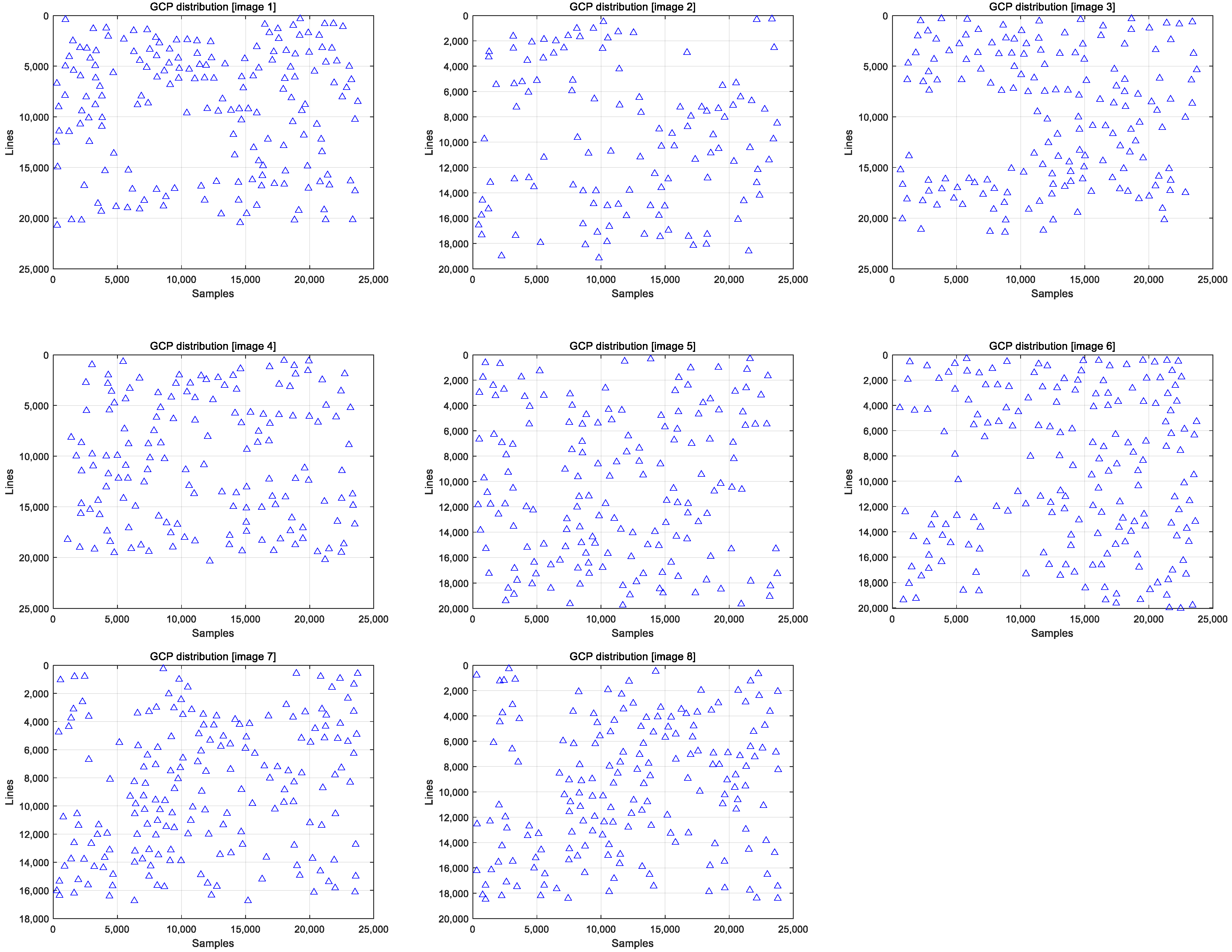
Figure 12.
The resulted GCP information for a total of eight Kompsat-3A target images (triangles: GCP).
Figure 12.
The resulted GCP information for a total of eight Kompsat-3A target images (triangles: GCP).

Figure 13.
Error pattern of each Kompsat-3A target image (left: column coordinates error, right: row coordinates error).
Figure 13.
Error pattern of each Kompsat-3A target image (left: column coordinates error, right: row coordinates error).


Figure 14.
Distribution of GCPs and check points (triangles: GCP, circle: check).

Figure 15.
Error change in RMSE for the number of GCP zones.

Figure 16.
Error histogram for the number of GCP zones (Image 3).

Figure 17.
Sub-cases of the three GCP zone.

Figure 18.
Error histogram for sub-cases of the three GCP zone.


Table 1.
Tested Kompsat-3A data specifications.
| Kompsat-3A | |
|---|---|
| Num of scenes | 8 |
| Date | 18 October 2015, 28 October 2015, 7 July 2018, 2 January 2019, 20 January 2019 (two scenes), 20 October 2020, 25 November 2020 |
| Azimuth/Off-nadir (degrees) | 262.6/27.8, 166.1/24.1, 261.2/9.8, 187.8/20.9, 181.8/22.4, 181.8/22.4, 197.4/33.3, 190.1/27.6 |
| GSD (m) | 0.73/0.63, 0.61/0.68, 0.56/0.55, 0.60/0.64, 0.60/0.65, 0.60/0.65, 0.72/0.78, 0.64/0.70 |
| Scene size (pixels) | 24,060 (width) × 17,000~24,080 (height) |
| Coverage | About 16 km × 13~16 km |
Table 2.
Aerial orthoimage and DSM.
| Aerial Orthoimage and DSM | |
|---|---|
| No. of aerial scenes | 132 |
| GSD (m) | 25 cm (aerial); 5 m (DSM) |
| Aerial image size (pixels) | 9396 × 11,520 |
Table 3.
Number of automatically generated GCPs.
| Kompsat-3A ID | Number |
|---|---|
| 1 | 175 |
| 2 | 115 |
| 3 | 160 |
| 4 | 149 |
| 5 | 162 |
| 6 | 180 |
| 7 | 181 |
| 8 | 175 |
| Mean | 162 |
Disclaimer/Publisher’s Note: The statements, opinions and data contained in all publications are solely those of the individual author(s) and contributor(s) and not of MDPI and/or the editor(s). MDPI and/or the editor(s) disclaim responsibility for any injury to people or property resulting from any ideas, methods, instructions or products referred to in the content. |
© 2024 by the authors. Licensee MDPI, Basel, Switzerland. This article is an open access article distributed under the terms and conditions of the Creative Commons Attribution (CC BY) license (https://creativecommons.org/licenses/by/4.0/).
Share and Cite
MDPI and ACS Style
Jo, H.; Lee, C.; Oh, J. The Impact of GCP Chip Distribution on Kompsat-3A RPC Bias Compensation. Appl. Sci. 2024, 14, 3482. https://doi.org/10.3390/app14083482
AMA Style
Jo H, Lee C, Oh J. The Impact of GCP Chip Distribution on Kompsat-3A RPC Bias Compensation. Applied Sciences. 2024; 14(8):3482. https://doi.org/10.3390/app14083482
Chicago/Turabian StyleJo, Hyeonjeong, Changno Lee, and Jaehong Oh. 2024. "The Impact of GCP Chip Distribution on Kompsat-3A RPC Bias Compensation" Applied Sciences 14, no. 8: 3482. https://doi.org/10.3390/app14083482
Note that from the first issue of 2016, this journal uses article numbers instead of page numbers. See further details here.