Method for the Experimental Identification of Variables and Configurations That Modify the Shape of the Macroscopic Fundamental Diagram

Abstract

In this paper, we propose a method for establishing if a variable is capable of modifying the Macroscopic Fundamental Diagram (MFD) of a street network. The variables have many different configurations, and a simulation is performed for each one. Then, based on the output data of each simulation, the representative speed, density, and flow of the network are calculated. We use three metrics to establish if a variable affects the MFD: the first establishes a distance between the compared density and speed patterns, the second establishes a distance between capacities, and the third establishes a distance between critical densities. We select four variables to test our method: the precision of driving, the vehicles’ top speeds distribution, the procedure for selecting routes, and the procedure for selecting destinations; we determine whether each of these variables can modify the MFD shape. Additionally, we detect which configurations of a variable are able to reach and exceed the critical density (causing congestion) so we can establish which configurations are sustainable and which are not. The novelties of this work are twofold: (1) we introduce a method to detect if a variable modifies the MFD; (2) we establish if the selected variables modify the MFD.

1. Introduction

The traffic performance of a network, based on traffic metrics that describe the whole network, is investigated via the macroscopic fundamental diagram (MFD). Proof of its existence (independently of the demand) is described in [1]. Some important findings of references [1,2,3] are that the MFD is a property of the network itself (i.e., its control and infrastructure) and not of the demand, and that the maximum flow is associated with a density value (the critical density) independently of the origin–destination table. In [3], the network MFD presents less scatter than the one that focuses on individual links. Also, the MFD reveals a well-defined, smoothly declining curve, considering the speeds and densities observed at different times of day and between multiple days. In [4], it was observed that when the flow vs. speed data of individual fixed detectors were aggregated, the scatter nearly disappeared in the resultant plot (a well-defined curve). Also, regularity conditions were proposed (though they were determined to be not necessary) in relation to the existence of the MFD. These included (i) slow-varying and distributed demand, (ii) a redundant network (with several route options), (iii) a homogeneous network (with similar links), and (iv) links with an approximate fundamental diagram. The relationship between production (average flow) with accumulation (average density) and the spatial inhomogeneity of density is presented in [5]. In this paper, the authors explain the nucleation effect (in which congestion concentrates in the bottlenecks that first appear and then propagates from these bottlenecks) and presents the relation of the standard deviation of density to production and with accumulation. If simulations start with homogeneous distribution of vehicles, uniform demand, and the same control for traffic lights, different spatial distribution of congestion can be observed due to the randomized turning of vehicles at intersections [6]. A sufficient condition for the existence of low-scatter MFD in arterial networks is described in [7]: if the spatial distribution of link density is the same for two time intervals with the same number of vehicles in the network, then the average flows should also be the same; nevertheless, no well-defined MFD was observed for the freeway network study case. Freeway networks do not have well-defined MFDs (density vs. flow) [8]. Freeway networks are different from arterial networks because they do not have traffic signals, are not redundant, and because of their transient states. The identified causes for freeways being hysteretic and path-dependent were different spatial heterogeneity in vehicle density in the onset and offset of congestion and capacity drop phenomena during the congestion offset (with lower flows at occupancy values near the critical point). The MFD on freeways was investigated in [9]. the relationship between vehicle hours traveled (VHT) and vehicle kilometers traveled (VKT) presents a well-defined shape (with no scatter) if all the links, and all the lanes of each link, are in the same regime (congested or uncongested); as the best performance (the higher VHT) on a freeway happens when all links (and all lanes) are under the same regime, policies to homogeneously spread congestion can be useful for maximizing the number of completed trips. The existence of well-defined MFDs was observed through clustering the zone under study in [10]. The partitioning mechanism consisted of applying three algorithms: segmenting, merging, and boundary adjustment. The resultant clusters had low density variation in the links and high spatial compactness. The time-varying nature of travel demands can induce scattering in the MFD, and appropriate boundary conditions (adjustments in the rationing of travel demand) are required to obtain a well-defined MDF, as demonstrated in [11]. In another study, two stochastic fundamental diagram (SFD) models with lognormal and skew-normal distributions were developed to account for the scattering effect during traffic state variations [12].

The MFD describes the behavior of a network in terms of its density, speed, and flow; if a network has a MDF (i.e., the relationships between traffic indicators present well-defined shapes), it can be used to identify the current conditions, to project future conditions, and to implement (control) actions that benefit the network’s traffic performance. Nevertheless, a network does not always present a well-defined MFD, and a hysteresis effect may be observed. An event that leads drivers to use unfamiliar routes can cause a hysteresis loop in the MFD [13]; during congestion recovery, a lesser flow is experienced compared to that observed during the congestion stage, since the more congested areas recover more slowly than those that are less congested. The effects of the hysteresis loop can be mitigated if drivers adaptively select routes. An incident originating a non-homogeneous congestion evolution in the network space can produce a hysteresis-like effect [14]. If an incident occurs in the centermost part of the surface streets, the hysteresis effect will not be visible in the MFD, but incidents that occur at other locations in the surface streets will be visible. Therefore, it was found to be convenient to separate surface streets (which were separated by the centermost streets and the rest) and highways (which were separated by penetrating roads and ring roads) in order to obtain MFDs with low scatter. The hysteresis phenomenon is explained as a consequence of departure time choices and user equilibrium in [15].

The MFD shape has been described using different methods. The MFDs obtained using the analytical method, the production method (based on the vehicles’ trajectories), and using loop detectors were compared in [16]. An algorithm that combines the data obtained with loop detector data (LDD) and floating car data (FCD) to estimate the MFD is presented in [17]. The problem of defining the MFD with probe vehicles when the penetration market rate of these varies regionally within a network was solved in [18]. Methods to estimate the MFD were compared and presented in [19]. The analytical method is suitable for an urban corridor and homogeneous loadings, and the typical route method was found to be adequate to obtain the network MFD in a grid network. A comparison between the method of cuts (MoC) and the stochastic approximation (SA) was implemented to analytically obtain the MFD in [20]. The MoC (a deterministic method) accurately found the upper bound of the MFD, whereas the SA (a stochastic method) provided a more accurate approximation of the MFD free-flow branch. A validity domain (and the inaccuracies) of the accumulation-based model when demand varied rapidly is described in [21]. The production with the accumulation and the spatial spread of density was modeled in [22]. The model describes the so-called generalized macroscopic fundamental diagram (GMFD). A functional form of the MFD called the uMFD (a smooth approximation of an upper bound of technologically feasible traffic states) was introduced in [23]; the uMFD fits the MFD’s empirical data through a trapezoidal shape, with four parameters considered to be physically meaningful. A novelty of this method is its use of the smoothing parameter, which allows quantification of the flow-reducing factors (infrastructure effects, vehicles interaction, and traffic heterogeneity). A two-step MFD calibration framework was used to select the form and to estimate parameters in [24].

Recently, the study of the MFD has been complemented by identifying the variables that modify the shape of the MFD. Interesting conclusions about the factors that affect the MFD shape were drawn in [25], which stated that ramp metering affects the MFD. When ramp metering was implemented, higher flows were observed for accumulation values after capacity, and without it, higher accumulation values were reached. The onset and offset of congestion can produce loops (even more than one), and rapid changes in demand affect the MFD. When the demand decreased sharply, lower flows were observed in the congestion recovery than during the congestion evolution (when accumulation was increasing). A bifurcation in the MFD (average network density vs. average network flow) was detected (considering weekdays) in [26]; in the MFD, a pattern in the morning peak and a different pattern in the evening peak could be distinguished. The identified cause of the bifurcation was that in the morning, drivers follow an efficient path (likely because they are going to work), and in the evening drivers take detours. In an arterial signalized intersection, a different capacity value was observed in the AM peak than in the PM peak [27]. The reasons for this were the ratio between green time and the traffic cycle time, signal coordination, and turning movements. Also, it was found that the scatter in the arterial fundamental diagram (AFD, represented as occupancy vs. flow) disappears if the Queue-Over-Detector (QOD, which is the phenomenon in which a vehicle is over the detector because the queue formed during the red time) is removed. In the absence of QOD, a stable AFD appears with three identifiable regimes: under-saturation, saturation, and over-saturation. The result of modifying the cycle length (or the offset) is that the MFD capacity changes [28]. The relation between accumulation and the trip completion rate was investigated in [29], an analytically derived Markov Chain framework was proposed to explain aggregate network dynamics, which was capable of accounting for uncertainties. The shape of an MFD (traffic density per unit of area vs. space mean speed over a time period) depends on the network’ topologies, as was evidenced in [30] with 63 networks; the space mean speed was explained with the macroscopic Underwood model, which has as parameters the free-flow space mean speed and the optimal traffic density per unit of area. These are explained in turn with the average number of junctions per unit distance (which captures the stop-and-go frequency of the vehicles) and with the degree density normalized by the trafficable area (which captures the intensity of conflicts between vehicles), respectively. The relation between the MFD properties and the structure of the road network is described [31]. The effects of signal coordination on the MFD were investigated in [32], which stated that the impacts of the strategies were sensitive to the signal cycle length chosen (60 s, 90 s, 120 s), and a poor signal coordination reduces the network capacity and the free-flow speed. Other variables that affect the MFD include junction regulation [33], traffic signals [34,35,36], network spatial characteristics [37], buses [38], large-scale activities [39], autonomous vehicles [40,41,42,43], turning traffic [44], rainfall [45], ride pooling [46], bicycle traffic [47], traffic incidents [48], the position of the loop detectors [49], and network heterogeneity [50].

As presented in the literature above, there are a lot of variables that can impact the MFD. However, a method to establish if a variable has impacts on the MFD is lacking. Moreover, it has yet to be determined which variables from a selected set affect the MFD. Thus, the aim of this work is to design a method to determine if a proposed variable modifies the MFD shape. A brief introduction of the method is as follows. For each variable selected, an experiment is conducted. During each experiment, a simulation is performed for each value (or configuration) the variable takes, and a MFD model is constructed with the aggregated data from each simulation. We compare the simulations by establishing a metric distance between density vs. speed patterns, between capacities, and between critical densities. The metrics are compared with thresholds values (these can be adjusted in order to increase or decrease the level of similarity pursued) and based on the global results, it can be concluded if a variable affects the MFD or not. If the latter applies, it means that (approximately) a unique MFD exists (density vs. speed, speed vs. flow, and density vs. flow) with the aggregated data from simulations (each performed with a different configuration of the variable) and that it can be used to describe the traffic.

Research Questions

As the study of the MFD is still underway, it has yet to be completely determined which variables affect the MFD shape of a network. Therefore, it becomes important to establish a method which allows us to analyze if a variable modifies the MFD shape. Thus, our research questions are as follows:

• What method can be used to analyze if a variable modifies the MFD shape of a street network?
• Are the precision of driving, the vehicles’ top speeds distribution, the procedure for selecting routes, and the procedure for selecting destinations variables that modify the MFD shape?

2. Materials and Methods

2.1. Simulator

In this study, we perform four experiments. In each experiment, a specific variable takes different values, and one simulation is performed for each value. To carry out the simulation, we use the Simulation of Urban Mobility (SUMO) version 1.15.0, a software which allows us to continuously simulate vehicular traffic at the microscopic level. We chose SUMO because it is a software that is open-source, free, and supports a space-continuous, time-discrete approach. In [51], the authors present simulations from three simulators (SUMO, VISSIM, and TRANSIMS), and the advantages and disadvantages of each are described. SUMO is used to create scenarios with different demand variations and supply disruptions in [52], in which the authors propose new indicators derived from the MFD to assess the traffic resilience in light of transportation system disruptions.

2.1.1. Vehicles Parameters

The default values of the vehicles’ parameters within the simulations are described in this section. By default, sigma = 0.5 which is the driver imperfection. It varies in the range of 0 to 1, with 0 indicating perfect driving and 1 indicating the opposite. By default, speedFactor = “normc(mean,deviation,lowerCutOff,upperCutOff)” = “normc(1,0.1,0.7,1.3)”, where speedFactor is a value that comes from a normal distribution with mean = 1, standard deviation = 0.1, lowerCutOff = 0.7, and upperCutOff = 1.3. The top speed of a vehicle is calculated as top_speed = normal_speed $\times$ speedFactor, with normal_speed = 16.6666 m/s, and speedFactor being a value in the range 0.7 to 1.3. In this study, the parameters sigma and speedFactor are selected and an experiment is performed for each. Thus, sigma is associated with the precision of driving in one experiment and speedFactor is associated with the vehicles’ top speeds distribution in other. These variables take different values in the simulations of their respective experiments.

The default values of the following parameters never change: vClass = “passenger”, length = 5 m (the vehicle length), minGap = 2.5 m (the minimum gap between vehicles at rest), accel = 2.6 m/s² (acceleration ability), decel = 4.5 m/s² (deceleration ability), emergencyDecel = 9 m/s² (emergency deceleration), and tau = 1 s (the driver’s desired minimum time headway). The parameter vClass = “passenger” indicates that the default SUMO parameters’ values for a passenger car (presented above) will be used; sigma and tau are parameters of the Krauß Car-following model (with modifications), which is the default Car-following model in SUMO.

Our intention is to select the parameters’ values so likely traffic conditions can emerge. For this reason, we choose the default SUMO parameters’ values as the base configuration for the simulations. Nevertheless, the parameters can be adjusted with empirical data for modeling observed traffic.

2.1.2. Routes and Destinations

By default, in a simulation, the vehicles’ routes are selected by considering the links’ travel times, which are calculated using the speed measurements of the previous period (1 period = 90 s). SUMO uses the Dijkstra algorithm to calculate the route with the shortest travel time. Also, by default, the origin–destination (OD) table is generated considering that each destination has the same probability of occurring, and it is guaranteed that each destination will be selected the same number of times. We consider the procedures for selecting routes and destinations as variables based upon which to perform experiments. Then, in one experiment, we manipulate the procedure for generating routes, i.e., we change the configuration of this variable, and in another we manipulate the procedure for generating destinations.

2.1.3. Network Speed

In a simulation, every 90 s (considering steps of 1 s to acquire data), we compute the network speed, density, and the flow of each link to build the network’s MFD. The speed on link x at time t is calculated using Equation (1),

$${\mathrm{I}\mathrm{N}\mathrm{S}\mathrm{T}\_\mathrm{s}\mathrm{p}\mathrm{e}\mathrm{e}\mathrm{d}}_{\mathrm{t}}^{\mathrm{x}}=\frac{1}{{\mathrm{N}}_{\mathrm{t}}^{\mathrm{x}}}{\sum }_{\mathrm{i}=1}^{\mathrm{i}={\mathrm{N}}_{\mathrm{t}}^{\mathrm{x}}}{\mathrm{v}\mathrm{e}\mathrm{h}\_\mathrm{s}\mathrm{p}\mathrm{e}\mathrm{e}\mathrm{d}}_{\mathrm{i}}^{\mathrm{t}}$$

(1)

where ${\mathrm{N}}_{\mathrm{t}}^{\mathrm{x}}$ is the number of vehicles on link x at time t and ${\mathrm{v}\mathrm{e}\mathrm{h}\_\mathrm{s}\mathrm{p}\mathrm{e}\mathrm{e}\mathrm{d}}_{\mathrm{i}}^{\mathrm{t}}$ is the speed of the i vehicle at time t. The representative speed of link x at period T is named ${\mathrm{P}\mathrm{E}\mathrm{R}\_\mathrm{s}\mathrm{p}\mathrm{e}\mathrm{e}\mathrm{d}}_{\mathrm{T}}^{\mathrm{x}}$ and is calculated using Equation (2) (expressed as pseudocode),

$\begin{array}{l}{\mathrm{P}\mathrm{E}\mathrm{R}\_\mathrm{s}\mathrm{p}\mathrm{e}\mathrm{e}\mathrm{d}}_{\mathrm{T}}^{\mathrm{x}}=0;\mathrm{k}=0\\ \mathrm{For}\mathrm{t}={\mathrm{t}}_1\mathrm{to}\mathrm{t}={\mathrm{t}}_2:\\ \mathrm{if}{\mathrm{N}}_{\mathrm{t}}^{\mathrm{x}}>0:\\ {\mathrm{P}\mathrm{E}\mathrm{R}\_\mathrm{s}\mathrm{p}\mathrm{e}\mathrm{e}\mathrm{d}}_{\mathrm{T}}^{\mathrm{x}}={\mathrm{P}\mathrm{E}\mathrm{R}\_\mathrm{s}\mathrm{p}\mathrm{e}\mathrm{e}\mathrm{d}}_{\mathrm{T}}^{\mathrm{x}}+{\mathrm{I}\mathrm{N}\mathrm{S}\mathrm{T}\_\mathrm{s}\mathrm{p}\mathrm{e}\mathrm{e}\mathrm{d}}_{\mathrm{t}}^{\mathrm{x}}\\ \mathrm{k}=\mathrm{k}+1\\ {\mathrm{P}\mathrm{E}\mathrm{R}\_\mathrm{s}\mathrm{p}\mathrm{e}\mathrm{e}\mathrm{d}}_{\mathrm{T}}^{\mathrm{x}}={\mathrm{P}\mathrm{E}\mathrm{R}\_\mathrm{s}\mathrm{p}\mathrm{e}\mathrm{e}\mathrm{d}}_{\mathrm{T}}^{\mathrm{x}}/\mathrm{k}\end{array}$

(2)

where k is the number of ${\mathrm{I}\mathrm{N}\mathrm{S}\mathrm{T}\_\mathrm{s}\mathrm{p}\mathrm{e}\mathrm{e}\mathrm{d}}_{\mathrm{t}}^{\mathrm{x}}$ measurements in the period T (ranging from t₁ to t₂) for which ${\mathrm{N}}_{\mathrm{t}}^{\mathrm{x}}>0$. When a simulation starts, the time is initiated at 0 s. The first period (T = 1) considers the period of time in the range [1 s, 90 s], the second period (T = 2) considers the period of time in the range [91 s, 180 s], and so on (units in seconds). Any period considers 90 steps of 1 s. Each 1 s (a time step) is attempted to calculate ${\mathrm{I}\mathrm{N}\mathrm{S}\mathrm{T}\_\mathrm{s}\mathrm{p}\mathrm{e}\mathrm{e}\mathrm{d}}_{\mathrm{t}}^{\mathrm{x}}$, and therefore the maximum value of k can be 90. Finally, the network’s speed at period T is calculated using Equation (3),

$${\mathrm{N}\mathrm{E}\mathrm{T}\_\mathrm{s}\mathrm{p}\mathrm{e}\mathrm{e}\mathrm{d}}_{\mathrm{T}}=\frac{1}{\mathrm{M}}{\sum }_{\mathrm{x}=1}^{\mathrm{x}=\mathrm{M}}{\mathrm{P}\mathrm{E}\mathrm{R}\_\mathrm{s}\mathrm{p}\mathrm{e}\mathrm{e}\mathrm{d}}_{\mathrm{T}}^{\mathrm{x}}$$

(3)

where M is the number of links considered for the analysis. The network speed, i.e., ${\mathrm{N}\mathrm{E}\mathrm{T}\_\mathrm{s}\mathrm{p}\mathrm{e}\mathrm{e}\mathrm{d}}_{\mathrm{T}}$, is the representative speed of the network at period T.

2.1.4. Network Density

The density on link x at time t is calculated using Equation (4),

$${\mathrm{M}\mathrm{E}\mathrm{A}\mathrm{S}\_\mathrm{d}\mathrm{e}\mathrm{n}\mathrm{s}\mathrm{i}\mathrm{t}\mathrm{y}}_{\mathrm{t}}^{\mathrm{x}}={\mathrm{N}}_{\mathrm{t}}^{\mathrm{x}}/({\mathrm{l}\mathrm{i}\mathrm{n}\mathrm{k}\_\mathrm{l}\mathrm{a}\mathrm{n}\mathrm{e}\mathrm{s}}^{\mathrm{x}}\ast {\mathrm{l}\mathrm{i}\mathrm{n}\mathrm{k}\_\mathrm{l}\mathrm{e}\mathrm{n}\mathrm{g}\mathrm{t}\mathrm{h}}^{\mathrm{x}})$$

(4)

where ${\mathrm{N}}_{\mathrm{t}}^{\mathrm{x}}$ is the number of vehicles on link x at time t, ${\mathrm{l}\mathrm{i}\mathrm{n}\mathrm{k}\_\mathrm{l}\mathrm{a}\mathrm{n}\mathrm{e}\mathrm{s}}^{\mathrm{x}}$ is the number of lanes of link x, and ${\mathrm{l}\mathrm{i}\mathrm{n}\mathrm{k}\_\mathrm{l}\mathrm{e}\mathrm{n}\mathrm{g}\mathrm{t}\mathrm{h}}^{\mathrm{x}}$ is the length of link x. The density of link x at period T is named ${\mathrm{P}\mathrm{E}\mathrm{R}\_\mathrm{d}\mathrm{e}\mathrm{n}\mathrm{s}\mathrm{i}\mathrm{t}\mathrm{y}}_{\mathrm{T}}^{\mathrm{x}}$ and is calculated using Equation (5) (expressed as pseudocode):

$\begin{array}{l}{\mathrm{P}\mathrm{E}\mathrm{R}\_\mathrm{d}\mathrm{e}\mathrm{n}\mathrm{s}\mathrm{i}\mathrm{t}\mathrm{y}}_{\mathrm{T}}^{\mathrm{x}}=0;\mathrm{k}=0\\ \mathrm{For}\mathrm{t}={\mathrm{t}}_1\mathrm{to}\mathrm{t}={\mathrm{t}}_2:\\ \mathrm{if}{\mathrm{N}}_{\mathrm{t}}^{\mathrm{x}}>0:\\ {\mathrm{P}\mathrm{E}\mathrm{R}\_\mathrm{d}\mathrm{e}\mathrm{n}\mathrm{s}\mathrm{i}\mathrm{t}\mathrm{y}}_{\mathrm{T}}^{\mathrm{x}}={\mathrm{P}\mathrm{E}\mathrm{R}\_\mathrm{d}\mathrm{e}\mathrm{n}\mathrm{s}\mathrm{i}\mathrm{t}\mathrm{y}}_{\mathrm{T}}^{\mathrm{x}}+{\mathrm{M}\mathrm{E}\mathrm{A}\mathrm{S}\_\mathrm{d}\mathrm{e}\mathrm{n}\mathrm{s}\mathrm{i}\mathrm{t}\mathrm{y}}_{\mathrm{t}}^{\mathrm{x}}\\ \mathrm{k}=\mathrm{k}+1\\ {\mathrm{P}\mathrm{E}\mathrm{R}\_\mathrm{d}\mathrm{e}\mathrm{n}\mathrm{s}\mathrm{i}\mathrm{t}\mathrm{y}}_{\mathrm{T}}^{\mathrm{x}}={\mathrm{P}\mathrm{E}\mathrm{R}\_\mathrm{d}\mathrm{e}\mathrm{n}\mathrm{s}\mathrm{i}\mathrm{t}\mathrm{y}}_{\mathrm{T}}^{\mathrm{x}}/\mathrm{k}\end{array}$

(5)

where k is the number of ${\mathrm{M}\mathrm{E}\mathrm{A}\mathrm{S}\_\mathrm{d}\mathrm{e}\mathrm{n}\mathrm{s}\mathrm{i}\mathrm{t}\mathrm{y}}_{\mathrm{t}}^{\mathrm{x}}$ measurements in the period T for which ${\mathrm{N}}_{\mathrm{t}}^{\mathrm{x}}>0$. The network density at period T is calculated using Equation (6),

$${\mathrm{N}\mathrm{E}\mathrm{T}\_\mathrm{d}\mathrm{e}\mathrm{n}\mathrm{s}\mathrm{i}\mathrm{t}\mathrm{y}}_{\mathrm{T}}=\frac{1}{\mathrm{M}}{\sum }_{\mathrm{x}=1}^{\mathrm{x}=\mathrm{M}}{\mathrm{P}\mathrm{E}\mathrm{R}\_\mathrm{d}\mathrm{e}\mathrm{n}\mathrm{s}\mathrm{i}\mathrm{t}\mathrm{y}}_{\mathrm{T}}^{\mathrm{x}}$$

(6)

2.1.5. Network Flow

The flow of link x at period T is calculated using Equation (7),

$${\mathrm{P}\mathrm{E}\mathrm{R}\_\mathrm{f}\mathrm{l}\mathrm{o}\mathrm{w}}_{\mathrm{T}}^{\mathrm{x}}=\frac{1}{90}{\sum }_{\mathrm{t}=1}^{\mathrm{t}=90}{\mathrm{M}\mathrm{E}\mathrm{A}\mathrm{S}\_\mathrm{f}\mathrm{l}\mathrm{o}\mathrm{w}}_{\mathrm{t}}^{\mathrm{x}}$$

(7)

where ${\mathrm{M}\mathrm{E}\mathrm{A}\mathrm{S}\_\mathrm{f}\mathrm{l}\mathrm{o}\mathrm{w}}_{\mathrm{t}}^{\mathrm{x}}$ is the number of vehicles on link x at time t that were not on link x at time t − 1. The network flow at period T is calculated using Equation (8),

$${\mathrm{N}\mathrm{E}\mathrm{T}\_\mathrm{f}\mathrm{l}\mathrm{o}\mathrm{w}}_{\mathrm{T}}=\frac{1}{\mathrm{M}}{\sum }_{\mathrm{x}=1}^{\mathrm{x}=\mathrm{M}}{\mathrm{P}\mathrm{E}\mathrm{R}\_\mathrm{f}\mathrm{l}\mathrm{o}\mathrm{w}}_{\mathrm{T}}^{\mathrm{x}}$$

(8)

2.2. Experiments

We perform four experiments. For each one, a variable is selected to determine if the variable affects the shape of the MFD. In each experiment, the selected variable takes a different value (or configuration) for each simulation and the output data of the simulations are prepared for comparison. In the simulations of any experiment, there is an input flow during 5 h (or 200 periods, since a period = 90 s, and 5 h = 200 periods); from period 1 to period 40 (phase one), every 10 s, a vehicle arrives at each network entrance (low_flow = 0.1 veh/s per entrance); from period 41 to period 80 (phase two), every 8 s, a vehicle arrives at each entrance (medium_flow = 0.125 veh/s per entrance); from period 81 to period 200 (phase three), every 6 s, a vehicle arrives at each entrance (high_flow = 0.1666 veh/s per entrance). The output data of a simulation are modeled with a linear equation for the network density vs. network speed pattern and with a second-degree polynomial for the network speed vs. network flow and for the network density vs. network flow patterns, the equations are solved using the least squares technique. In the Supplementary Materials section, it can be found the link to the data and codes to reproduce our experiments.

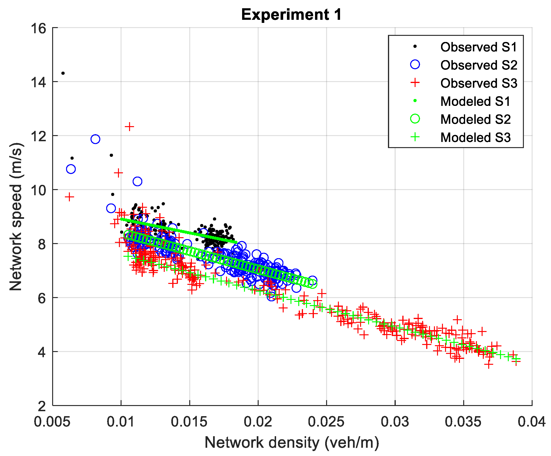
2.2.1. Experiment 1: The Precision for Driving

In this experiment, we performed three simulations. In simulation 1, the parameter sigma = 0; in simulation 2 sigma = 0.5; in simulation 3, sigma = 1. At this point, it should be mentioned that sigma = 0.5 (in between perfect driving and the most imperfect driving) is comparable with human driving behavior [41]. The network density vs. network speed pattern (for any simulation) was modeled with a linear equation of the form $\mathrm{y}=\mathrm{a}\mathrm{x}+\mathrm{b}$ and solved with regression analysis, where a and b are parameters, x = network density and y = network speed; the network speed vs. network flow pattern (for any simulation) was modeled with a polynomial equation of the second degree, i.e., $\mathrm{y}={\mathrm{x}}^2\mathrm{a}+\mathrm{x}\mathrm{b}+\mathrm{c}$ which was solved with regression analysis, where a, b, and c are parameters, x = network speed and y = network flow. The network density vs. network flow pattern (for any simulation) was modeled with a polynomial equation of the second degree, i.e., $\mathrm{y}={\mathrm{x}}^2\mathrm{a}+\mathrm{x}\mathrm{b}+\mathrm{c}$ which was solved with regression analysis, where a, b, and c are parameters, x = network density and y = network flow. To model the three patterns for any simulation, we considered a range of periods [3, 202], since at the beginning of a simulation, links are starting to fill up, whereas they become empty towards the end.

Hereafter, simulation 1 is abbreviated as S1, simulation 2 is S2, and simulation 3 is S3. We establish if network density vs. network speed (DS) patterns are similar using Equation (9), which is presented with the example for calculating the distance between the modeled DS patterns of simulation 1 and simulation 2,

$${\mathrm{D}}_{\mathrm{s}\mathrm{p}\mathrm{e}\mathrm{e}\mathrm{d}}^{\mathrm{S}1\mathrm{S}2}=\frac{1}{\mathrm{N}}{\sum }_{\mathrm{i}=1}^{\mathrm{i}=\mathrm{N}}\left|{\mathrm{y}}_{\mathrm{i}}^{\mathrm{S}2}-{\mathrm{y}}_{\mathrm{i}}^{\mathrm{S}1}\right|$$

(9)

where N is the number of points selected in the x-axis (network density values), i is the index for N values, superscripts S1, S2, and S3 stands for simulation 1, simulation 2, and simulation 3, respectively; then ${\mathrm{D}}_{\mathrm{s}\mathrm{p}\mathrm{e}\mathrm{e}\mathrm{d}}^{\mathrm{S}1\mathrm{S}2}$ is the speed distance between the modeled DS patterns of S1 and S2. In Equation (9), we can see the absolute value of the difference between the modeled network speed values of S1 and S2 for a certain network density value. As we are comparing S1 and S2, the x-axis values set of S1 is ${\mathrm{R}}^{\mathrm{S}1}=\{{\mathrm{x}}_1^{\mathrm{S}1},{\mathrm{x}}_2^{\mathrm{S}1},\dots {\mathrm{x}}_{\mathrm{N}1}^{\mathrm{S}1}\}$ and the x-axis values set of S2 is ${\mathrm{R}}^{\mathrm{S}2}=\{{\mathrm{x}}_1^{\mathrm{S}2},{\mathrm{x}}_2^{\mathrm{S}2},\dots {\mathrm{x}}_{\mathrm{N}2}^{\mathrm{S}2}\}$. With N1, for the number of network density values of S1 and N2 the number of network density values of S2, the values of these sets are ordered from the lowest to the highest. The x-axis set of values for comparing the y-axis values of S1 and S2 is $\left\{{\mathrm{x}}_1,{\mathrm{x}}_3,\dots ,{\mathrm{x}}_{\mathrm{N}}\right\}=\{\mathrm{x}:\mathrm{x}\in {\mathrm{R}}^{\mathrm{S}1}\cup {\mathrm{R}}^{\mathrm{S}2} \mathrm{a}\mathrm{n}\mathrm{d} {\mathrm{x}}_1\le \mathrm{x}\le {\mathrm{x}}_{\mathrm{N}}\}$, where ${\mathrm{x}}_1=\mathrm{m}\mathrm{a}\mathrm{x}({\mathrm{x}}_1^{\mathrm{S}1},{\mathrm{x}}_1^{\mathrm{S}2})$ and ${\mathrm{x}}_{\mathrm{N}}=\mathrm{m}\mathrm{i}\mathrm{n}({\mathrm{x}}_{\mathrm{N}1}^{\mathrm{S}1},{\mathrm{x}}_{\mathrm{N}2}^{\mathrm{S}2})$.

Based on Equation (9), we compare the DS patterns of two simulations. We compare S1 with S2, S2 with S3, and S1 with S3. When comparing the DS patterns of two simulations, a condition rule is established that depends on a threshold value. This value is intended to be flexible so it can be set according to the needs of an investigation (providing the rigor needed to distinguish DS patterns). We establish that if ${\mathrm{D}}_{\mathrm{s}\mathrm{p}\mathrm{e}\mathrm{e}\mathrm{d}}\le 1 \mathrm{m}/\mathrm{s}$ (in this example, the threshold value is 6% of the normal_speed, i.e., $16.66\frac{\mathrm{m}}{\mathrm{s}}\ast 0.06\cong 1\frac{\mathrm{m}}{\mathrm{s}}$) the following is true: there is no significant difference between the patterns. If ${\mathrm{D}}_{\mathrm{s}\mathrm{p}\mathrm{e}\mathrm{e}\mathrm{d}}>1 \mathrm{m}/\mathrm{s}$, there is a significant difference between the patterns. In addition, we define the difference in capacities between two simulations as ${\mathrm{D}}_{\mathrm{f}\mathrm{l}\mathrm{o}\mathrm{w}}^{\mathrm{S}1\mathrm{S}2}=\left|{\mathrm{c}\mathrm{a}\mathrm{p}\mathrm{a}\mathrm{c}\mathrm{i}\mathrm{t}\mathrm{y}}^{\mathrm{S}2}-{\mathrm{c}\mathrm{a}\mathrm{p}\mathrm{a}\mathrm{c}\mathrm{i}\mathrm{t}\mathrm{y}}^{\mathrm{S}1}\right|$ and the difference in critical densities as ${\mathrm{D}}_{\mathrm{d}\mathrm{e}\mathrm{n}\mathrm{s}\mathrm{i}\mathrm{t}\mathrm{y}}^{\mathrm{S}1\mathrm{S}2}=\left|{\mathrm{c}\mathrm{r}\mathrm{i}\mathrm{t}\mathrm{i}\mathrm{c}\mathrm{a}\mathrm{l}\_\mathrm{d}\mathrm{e}\mathrm{n}\mathrm{s}\mathrm{i}\mathrm{t}\mathrm{y}}^{\mathrm{S}2}-{\mathrm{c}\mathrm{r}\mathrm{i}\mathrm{t}\mathrm{i}\mathrm{c}\mathrm{a}\mathrm{l}\_\mathrm{d}\mathrm{e}\mathrm{n}\mathrm{s}\mathrm{i}\mathrm{t}\mathrm{y}}^{\mathrm{S}1}\right|$, where capacity^S is the maximum network flow from the modeled data of simulation S and cricital_density^S is the corresponding network density at capacity, with S = {S1, S2, S3}. We define two additional rules and select the threshold values. If ${\mathrm{D}}_{\mathrm{f}\mathrm{l}\mathrm{o}\mathrm{w}}\le 0.01 \mathrm{v}\mathrm{e}\mathrm{h}/\mathrm{s}$, there is no significant difference between the capacities of the simulations compared. The opposite is true if ${\mathrm{D}}_{\mathrm{f}\mathrm{l}\mathrm{o}\mathrm{w}}>0.01 \mathrm{v}\mathrm{e}\mathrm{h}/\mathrm{s}$; in this case, the threshold value is the 6% of high_flow, i.e., $\frac{1 \mathrm{v}\mathrm{e}\mathrm{h}}{6 \mathrm{s}}\times 0.06\cong 0.01\frac{\mathrm{veh}}{\mathrm{s}}$. If ${\mathrm{D}}_{\mathrm{d}\mathrm{e}\mathrm{n}\mathrm{s}\mathrm{i}\mathrm{t}\mathrm{y}}\le 0.002 \mathrm{v}\mathrm{e}\mathrm{h}/\mathrm{m}$, there is no significant difference between the critical densities of the simulations compared. The opposite is true if ${\mathrm{D}}_{\mathrm{d}\mathrm{e}\mathrm{n}\mathrm{s}\mathrm{i}\mathrm{t}\mathrm{y}}>0.002 \mathrm{v}\mathrm{e}\mathrm{h}/\mathrm{m}$; in this case, the threshold value is 20% of the high_flow divided by the normal_speed, i.e., $(\frac{1 \mathrm{v}\mathrm{e}\mathrm{h}}{6 \mathrm{s}}/16.66\frac{\mathbf{m}}{\mathrm{s}})\times 0.2\cong 0.002\frac{\mathrm{veh}}{\mathrm{m}}$. We establish that the MFDs of the compared simulations are dissimilar if at least two of the following three conditions are true: ${\mathrm{D}}_{\mathrm{s}\mathrm{p}\mathrm{e}\mathrm{e}\mathrm{d}}>1 \mathrm{m}/\mathrm{s}$, ${\mathrm{D}}_{\mathrm{f}\mathrm{l}\mathrm{o}\mathrm{w}}>0.01 \mathrm{v}\mathrm{e}\mathrm{h}/\mathrm{s}$, and ${\mathrm{D}}_{\mathrm{d}\mathrm{e}\mathrm{n}\mathrm{s}\mathrm{i}\mathrm{t}\mathrm{y}}>0.002 \mathrm{v}\mathrm{e}\mathrm{h}/\mathrm{m}$.

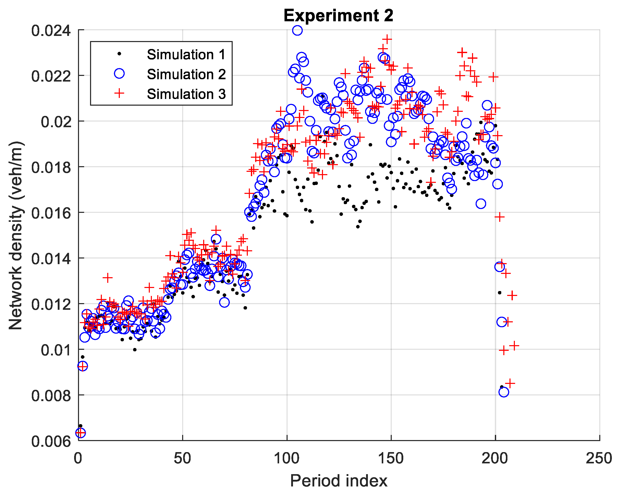
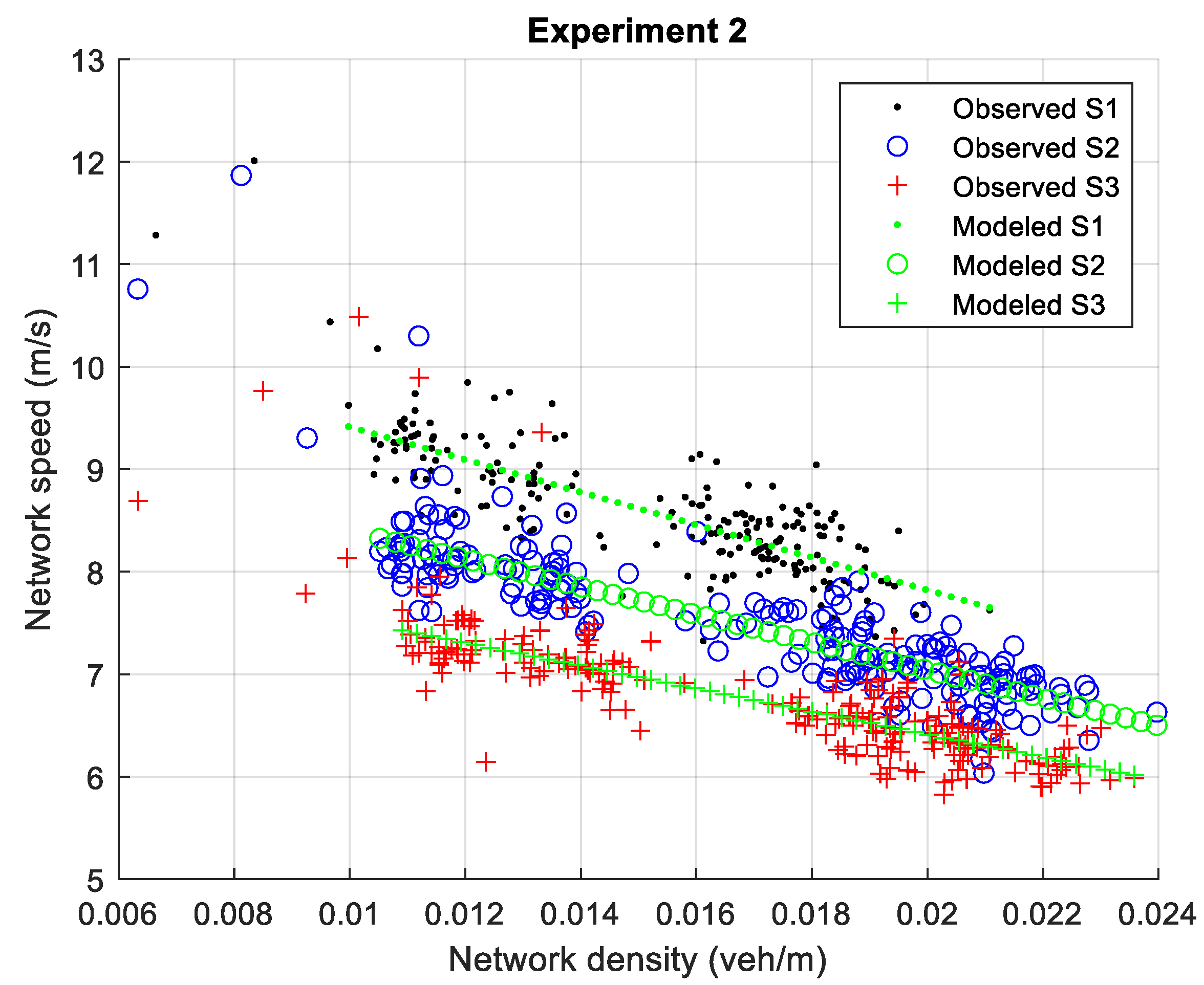
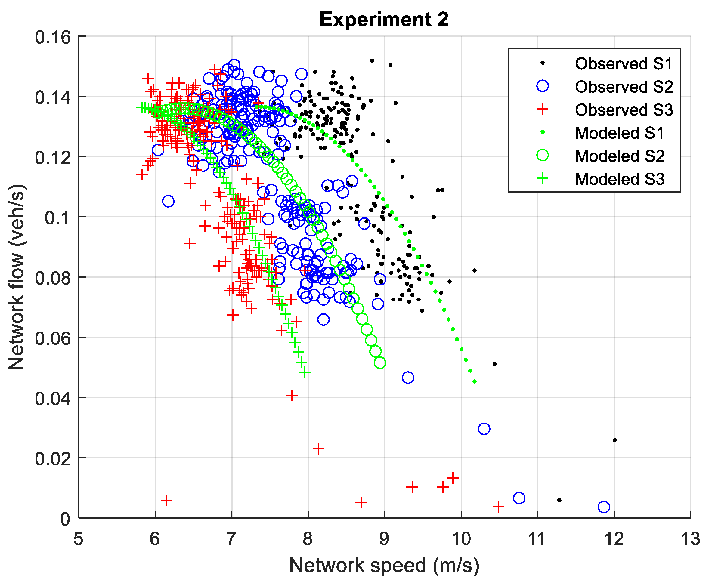
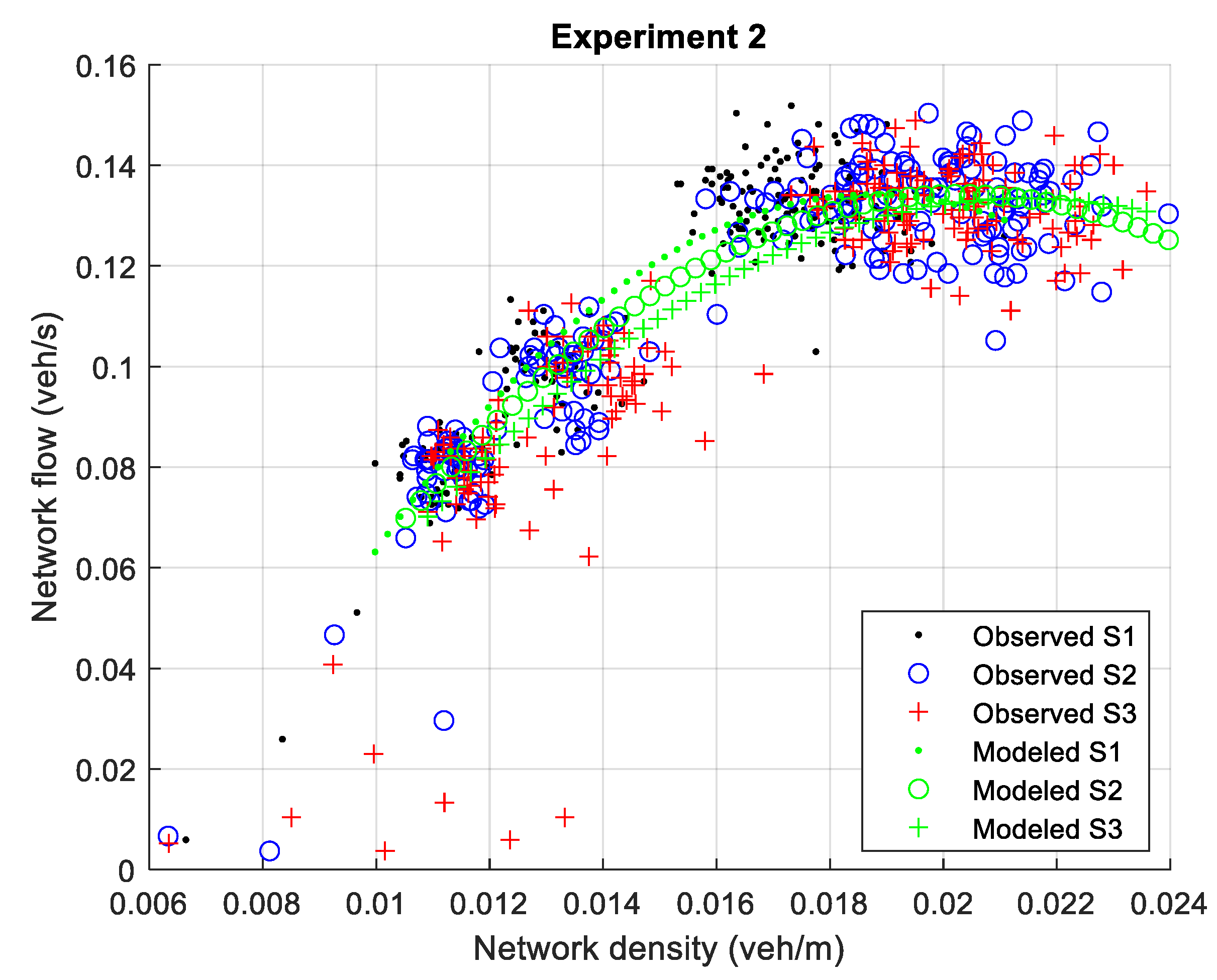
2.2.2. Experiment 2: The Vehicles’ Top Speeds Distribution

In this experiment, we performed three simulations. In the first simulation, the parameter speedFactor was set at “normc(1.15,0.05,1,1.3)”; in the second simulation, it was set at speedFactor=“normc(1,0.1,0.7,1.3)”; in the third simulation, it was set at speedFactor=“normc(0.85,0.05,0.7,1)”. S2 includes the widest range of top speeds, thus delivering a realistic situation for traffic conditions.

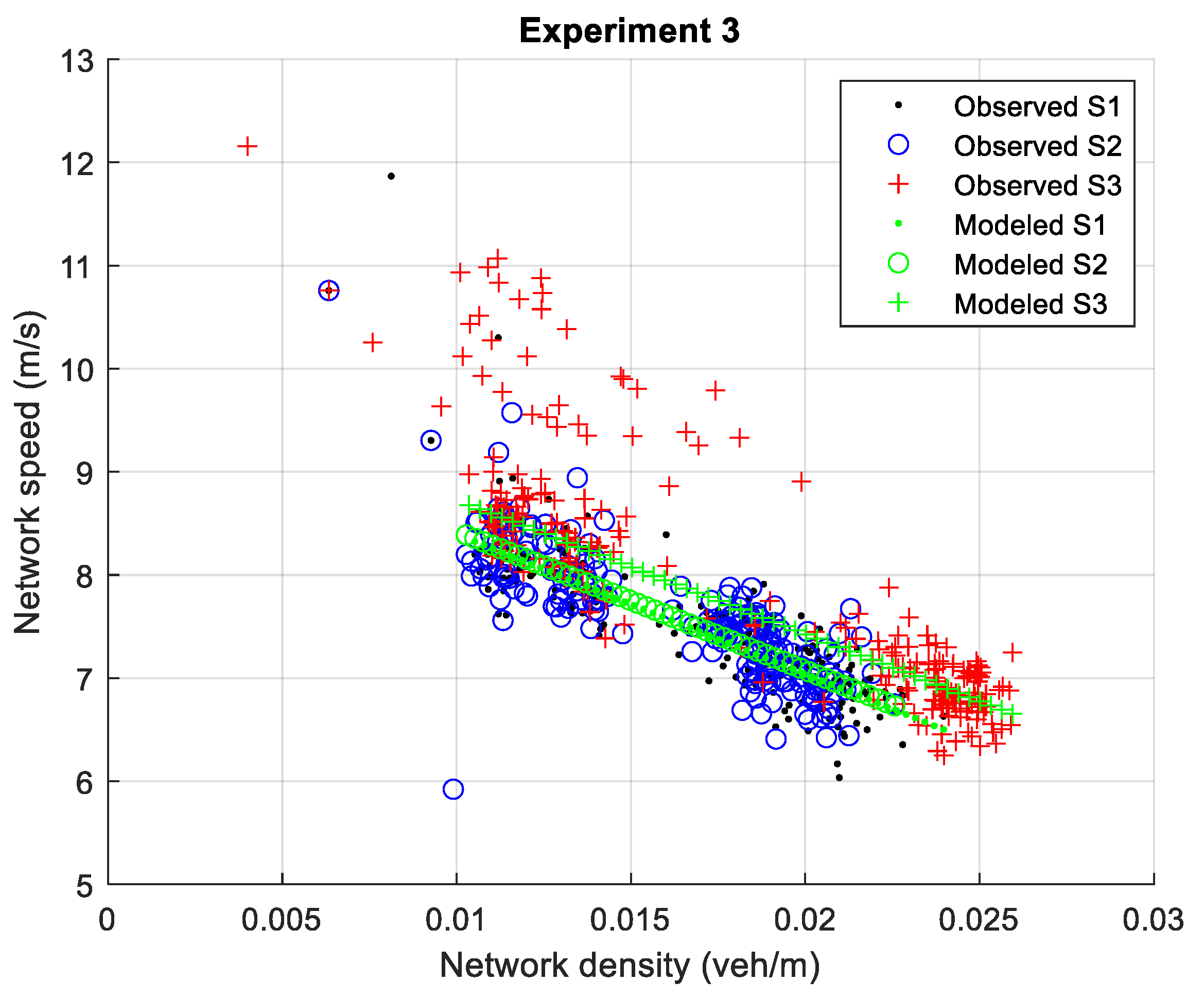
2.2.3. Experiment 3: The Procedure for Selecting Routes

In this experiment, we performed three simulations. In the first simulation, the vehicles routes were chosen with the links’ travel times calculated every 90 s based on the links speeds of the previous period, i.e., ${{\mathrm{t}\mathrm{r}\mathrm{a}\mathrm{v}\mathrm{e}\mathrm{l}\_\mathrm{t}\mathrm{i}\mathrm{m}\mathrm{e}}_{\mathrm{T}}^{\mathrm{x}}={\mathrm{l}\mathrm{i}\mathrm{n}\mathrm{k}\_\mathrm{l}\mathrm{e}\mathrm{n}\mathrm{g}\mathrm{t}\mathrm{h}}^{\mathrm{x}}/\mathrm{P}\mathrm{E}\mathrm{R}\_\mathrm{s}\mathrm{p}\mathrm{e}\mathrm{e}\mathrm{d}}_{\mathrm{T}-1}^{\mathrm{x}}$, with ${\mathrm{t}\mathrm{r}\mathrm{a}\mathrm{v}\mathrm{e}\mathrm{l}\_\mathrm{t}\mathrm{i}\mathrm{m}\mathrm{e}}_{\mathrm{T}}^{\mathrm{x}}$ being the representative travel time of segment x at any time t belonging to period T. In the second simulation, the links’ travel times were calculated every 90 s considering the links’ speeds of the previous two periods, i.e., ${\mathrm{t}\mathrm{r}\mathrm{a}\mathrm{v}\mathrm{e}\mathrm{l}\_\mathrm{t}\mathrm{i}\mathrm{m}\mathrm{e}}_{\mathrm{T}}^{\mathrm{x}}={\mathrm{l}\mathrm{i}\mathrm{n}\mathrm{k}\_\mathrm{l}\mathrm{e}\mathrm{n}\mathrm{g}\mathrm{t}\mathrm{h}}^{\mathrm{x}}/({(\mathrm{P}\mathrm{E}\mathrm{R}\_\mathrm{s}\mathrm{p}\mathrm{e}\mathrm{e}\mathrm{d}}_{\mathrm{T}-1}^{\mathrm{x}}+{\mathrm{P}\mathrm{E}\mathrm{R}\_\mathrm{s}\mathrm{p}\mathrm{e}\mathrm{e}\mathrm{d}}_{\mathrm{T}-2}^{\mathrm{x}})/2)$. In the third simulation, the travel time of each segment was a constant, so ${\mathrm{t}\mathrm{r}\mathrm{a}\mathrm{v}\mathrm{e}\mathrm{l}\_\mathrm{t}\mathrm{i}\mathrm{m}\mathrm{e}}_{\mathrm{T}}^{\mathrm{x}}={\mathrm{l}\mathrm{i}\mathrm{n}\mathrm{k}\_\mathrm{l}\mathrm{e}\mathrm{n}\mathrm{g}\mathrm{t}\mathrm{h}}^{\mathrm{x}}/\mathrm{n}\mathrm{o}\mathrm{r}\mathrm{m}\mathrm{a}\mathrm{l}\_\mathrm{s}\mathrm{p}\mathrm{e}\mathrm{e}\mathrm{d}$ for any T. For all simulations, the route of a vehicle was computed using the Dijkstra algorithm, which selects the route with the shortest travel time.

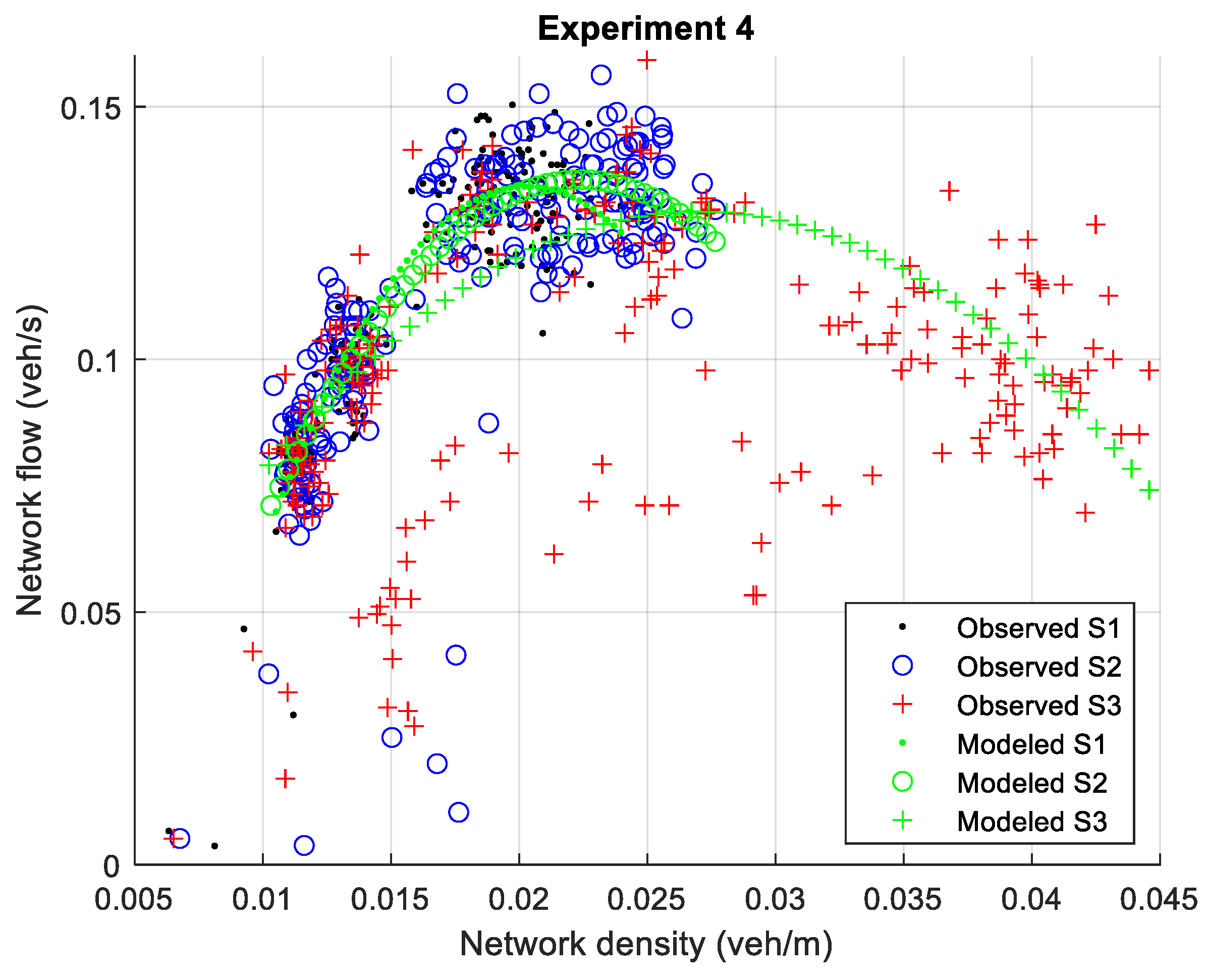
2.2.4. Experiment 4: The Procedure for Selecting Destinations

In this experiment, we performed three simulations. In S1, each destination had the same likelihood of being selected and it was guaranteed that each destination would be selected the same number of times. In S2, each destination had the same likelihood of being selected but it was not guaranteed that each destination would be selected the same number of times. Destinations with the same probability of being selected could favor (to some extent) the uniform distribution of vehicles in the network links (a desirable traffic situation). In S3, we randomly selected, in the range [0.5, 1], the probability of occurrence of each destination (i.e., a destination with a probability = 0.5 has the half of likelihood of occurring when compared to a destination with a probability = 1), so the probabilities of the destinations with ID 0 to ID 14 were 0.7, 0.7, 1.0, 0.6, 0.6, 1.0, 1.0, 0.8, 0.9, 0.8, 1.0, 0.7, 0.8, 0.5, 0.5, respectively. Then, the vehicles were assigned a destination according to the probabilities we set for that simulation.

3. Results and Discussion

3.1. Results and Discussion of Experiment 1

Figure 1, Figure 2 and Figure 3 present the period index vs. network speed, period index vs. network density, and period index vs. network flow, respectively; in these Figures, the black dots represent the data from simulation 1, the blue circles represent the data from simulation 2, and the red crosses represent the data from simulation 3.

Figure 4, Figure 5 and Figure 6 show the network density vs. network speed, network speed vs. network flow, and network density vs. network flow, respectively. These Figures present the data of each simulation. In addition, green dots represent the modeled pattern with the data of simulation 1, green circles represent the modeled pattern with the data of simulation 2, and green crosses represent the modeled pattern with the data of simulation 3.

We obtain ${\mathrm{D}}_{\mathrm{s}\mathrm{p}\mathrm{e}\mathrm{e}\mathrm{d}}^{\mathrm{S}1\mathrm{S}2}=0.6592 \mathrm{m}/\mathrm{s}$, ${\mathrm{D}}_{\mathrm{s}\mathrm{p}\mathrm{e}\mathrm{e}\mathrm{d}}^{\mathrm{S}2\mathrm{S}3}=0.7956 \mathrm{m}/\mathrm{s}$, and ${\mathrm{D}}_{\mathrm{s}\mathrm{p}\mathrm{e}\mathrm{e}\mathrm{d}}^{\mathrm{S}1\mathrm{S}3}=1.4486 \mathrm{m}/\mathrm{s}$, and therefore a sigma difference of 0.5 does not modify the DS pattern, but a sigma difference of 1 modifies the DS pattern. The DS patterns between S1 and S2 are similar, the DS patterns between S2 and S3 are similar, and the DS patterns between S1 (with sigma = 0) and S3 (with sigma = 1) are dissimilar. ${\mathrm{D}}_{\mathrm{f}\mathrm{l}\mathrm{o}\mathrm{w}}^{\mathrm{S}1\mathrm{S}2}=\left|0.138787-0.134236\right|=0.00455 \mathrm{v}\mathrm{e}\mathrm{h}/\mathrm{s}$, ${\mathrm{D}}_{\mathrm{f}\mathrm{l}\mathrm{o}\mathrm{w}}^{\mathrm{S}2\mathrm{S}3}=\left|0.134236-0.119678\right|=0.014557 \mathrm{v}\mathrm{e}\mathrm{h}/\mathrm{s}$, and ${\mathrm{D}}_{\mathrm{f}\mathrm{l}\mathrm{o}\mathrm{w}}^{\mathrm{S}1\mathrm{S}3}\left|0.138787-0.119678\right|=0.019108 \mathrm{v}\mathrm{e}\mathrm{h}/\mathrm{s}$, hence the capacities of S1 and S2 are similar, the capacities of S2 and S3 are dissimilar, and the capacities of S1 and S3 are dissimilar. ${\mathrm{D}}_{\mathrm{d}\mathrm{e}\mathrm{n}\mathrm{s}\mathrm{i}\mathrm{t}\mathrm{y}}^{\mathrm{S}1\mathrm{S}2}=\left|0.018376-0.0202025\right|=0.001826 \mathrm{v}\mathrm{e}\mathrm{h}/\mathrm{m}$, ${\mathrm{D}}_{\mathrm{d}\mathrm{e}\mathrm{n}\mathrm{s}\mathrm{i}\mathrm{t}\mathrm{y}}^{\mathrm{S}2\mathrm{S}3}=\left|0.0202025-0.0258002\right|=0.005597 \mathrm{v}\mathrm{e}\mathrm{h}/\mathrm{m}$, and ${\mathrm{D}}_{\mathrm{d}\mathrm{e}\mathrm{n}\mathrm{s}\mathrm{i}\mathrm{t}\mathrm{y}}^{\mathrm{S}1\mathrm{S}3}\left|0.018376-0.0258002\right|=0.007424 \mathrm{v}\mathrm{e}\mathrm{h}/\mathrm{m}$, hence the critical densities of S1 and S2 are similar, the critical densities of S2 and S3 are dissimilar, and the critical densities of S1 and S3 are dissimilar. The results presented above are summarized in

Table 1. Comparing simulations with metrics: experiment 1.

Compared Simulations	Comparing the Speed in a Density Range (m/s)	Comparing Capacity (veh/s)	Comparing Critical Density (veh/m)	MFDs Comparison Verdict
S1 and S2	${\mathrm{D}}_{\mathrm{s}\mathrm{p}\mathrm{e}\mathrm{e}\mathrm{d}}^{\mathrm{S}1\mathrm{S}2}=0.6592$ (similar)	${\mathrm{D}}_{\mathrm{f}\mathrm{l}\mathrm{o}\mathrm{w}}^{\mathrm{S}1\mathrm{S}2}=0.00455$ (similar)	${\mathrm{D}}_{\mathrm{d}\mathrm{e}\mathrm{n}\mathrm{s}\mathrm{i}\mathrm{t}\mathrm{y}}^{\mathrm{S}1\mathrm{S}2}=0.001826$ (similar)	Similar
S2 and S3	${\mathrm{D}}_{\mathrm{s}\mathrm{p}\mathrm{e}\mathrm{e}\mathrm{d}}^{\mathrm{S}2\mathrm{S}3}=0.7956$ (similar)	${\mathrm{D}}_{\mathrm{f}\mathrm{l}\mathrm{o}\mathrm{w}}^{\mathrm{S}2\mathrm{S}3}=0.014557$ (dissimilar)	${\mathrm{D}}_{\mathrm{d}\mathrm{e}\mathrm{n}\mathrm{s}\mathrm{i}\mathrm{t}\mathrm{y}}^{\mathrm{S}2\mathrm{S}3}=0.005597$ (dissimilar)	Dissimilar
S1 and S3	${\mathrm{D}}_{\mathrm{s}\mathrm{p}\mathrm{e}\mathrm{e}\mathrm{d}}^{\mathrm{S}1\mathrm{S}3}=1.4486$ (dissimilar)	${\mathrm{D}}_{\mathrm{f}\mathrm{l}\mathrm{o}\mathrm{w}}^{\mathrm{S}1\mathrm{S}3}=0.019108$ (dissimilar)	${\mathrm{D}}_{\mathrm{d}\mathrm{e}\mathrm{n}\mathrm{s}\mathrm{i}\mathrm{t}\mathrm{y}}^{\mathrm{S}1\mathrm{S}3}=0.007424$ (dissimilar)	Dissimilar

. According to these results, the precision for driving (sigma) is a variable that can affect the MFD; the MFDs between S2 and S3, and between S1 and S3, are dissimilar.

In

Table 2. Traffic indicators’ AVG and STD of S1, S2, and S3 in each phase: experiment 1.

Sim		Period 1 to 40	Period 41 to 80	Period 80 to 204
Simulation 1	AVG speed (m/s)	8.94926718872254	8.51797706960548	8.28313045186715
	STD speed (m/s)	0.509450884198832	0.396801577211994	0.661450465348051
	AVG density (veh/m)	0.0109832325877089	0.0129306974086639	0.0166717482607360
	STD density (veh/m)	0.000890871263263841	0.000600500246470353	0.00145233179687904
	AVG flow (veh/s)	0.0768888888888889	0.0995185185185185	0.130195329230631
	STD flow (veh/s)	0.0132393012187418	0.00659889579912034	0.0181354198974069
Simulation 2	AVG speed (m/s)	8.28993901306706	7.97190484356544	7.15742558895287
	STD speed (m/s)	0.524544738286513	0.289676483985101	0.641752021714726
	AVG density (veh/m)	0.0111114429629568	0.0132940390041025	0.0194440957389438
	STD density (veh/m)	0.000932282443886002	0.000697463548430562	0.00223166553880638
	AVG flow (veh/s)	0.0767777777777778	0.0993148148148148	0.130292712066906
	STD flow (veh/s)	0.0133750008423410	0.00715306455474556	0.0179194442178534
Simulation 3	AVG speed (m/s)	7.47604877652992	6.96968513152068	5.78687086950815
	STD speed (m/s)	0.477964209633950	0.331662461188288	1.67627926136163
	AVG density (veh/m)	0.0114605066447026	0.0145884916986345	0.0254291591795365
	STD density (veh/m)	0.00105492450138108	0.000798070643991101	0.00903979438586012
	AVG flow (veh/s)	0.0764259259259259	0.0988888888888889	0.0909404910528506
	STD flow (veh/s)	0.0141203692027462	0.00652912889373503	0.0359795272430116

, the mean (AVG) and standard deviation (STD) of the network speed, network density, and network flow for simulations S1, S2, and S3 in experiment 1 are presented across three phases.

In Figure 4, it can be observed that as the driving imperfection is set higher (i.e., as its value is increased from simulation 1 to simulation 3), a greater maximum density is reached, which also implies a lower minimum speed. Then, a simulation with a higher sigma value than other presents a lower minimum speed and a higher maximum density. In simulation 1, the maximum observed density is 0.0184 veh/m, in simulation 2, it is 0.024 veh/m, and in simulation 3, it is 0.0388 veh/m. In simulation 1, the minimum observed speed is 7.4179 m/s, in simulation 2, it is 6.0352 m/s, and in simulation 3, it is 3.526 m/s. The network density vs. network speed pattern of S1 is above the DS pattern of S2, and the DS pattern of S2 is above the DS pattern of S3, which indicates that for the density value, higher speed occurred in S1, followed by S2 and then S3.

The duration of simulations 1 and 2 was from period 1 to 204, whereas for simulation 3 it took place from period 1 to 258. During the simulations, we generated vehicles during the first 5 h (5 h = 200 periods, since 1 period = 90 s). In simulations 1 and 2, from period 200, it took an additional 4 periods (6 min) for the vehicles still circulating in the network to leave it, whereas in simulation 3, an additional 58 periods were required (87 min), since S3 experiences congestion (i.e., it reaches the critical density from which flow decreases; see Figure 6). This implies that queues are formed at the entry links (not all vehicles are able to enter the network at the time when are spawned, as dictated by the input flow) and that the network flow goes up and down during the congestion (in a period range when input flow = high_flow; see Figure 3). In Figure 6, it is appreciated that in S3, the critical density is reached at 0.0258 veh/m (according to the modeled data); Figure 2 shows that from approximately period 97 to 204 in S3, the critical density is surpassed (in that range, if density increases, flow decreases). From period 81 (i.e., since the input flow at each network entrance is equal to high_flow) it takes around 25.5 min (the time that elapses between period 81 and period 97) for the congestion to emerge; in the range of periods described in [97, 204], the speed is notoriously lower in S3 than in S1 and S2 (see Figure 1), the density is higher (see Figure 2), and the flow is (repeatedly) lower (see Figure 3).

3.2. Results and Discussion of Experiment 2

Figure 7, Figure 8 and Figure 9 present period index vs. network speed, period index vs. network density, and period index vs. network flow, respectively.

Figure 10, Figure 11 and Figure 12 show the network density vs. network speed, network speed vs. network flow, and network density vs. network flow, respectively.

The distance between the network density vs. network speed pattern of simulation 1 (in green dots) and the pattern of simulation 2 (in green circles) is ${\mathrm{D}}_{\mathrm{s}\mathrm{p}\mathrm{e}\mathrm{e}\mathrm{d}}^{\mathrm{S}1\mathrm{S}2}=0.8842 \mathrm{m}/\mathrm{s}$; between simulation 2 and simulation 3 (in green crosses), it is ${\mathrm{D}}_{\mathrm{s}\mathrm{p}\mathrm{e}\mathrm{e}\mathrm{d}}^{\mathrm{S}2\mathrm{S}3}=0.6974 \mathrm{m}/\mathrm{s}$; and between S1 and S3, it is ${\mathrm{D}}_{\mathrm{s}\mathrm{p}\mathrm{e}\mathrm{e}\mathrm{d}}^{\mathrm{S}1\mathrm{S}3}=1.5998 \mathrm{m}/\mathrm{s}$. Therefore, the DS patterns of S1 and S2 are similar, the DS patterns of S2 and S3 are similar, and the DS patterns of S1 and S3 are dissimilar. ${\mathrm{D}}_{\mathrm{f}\mathrm{l}\mathrm{o}\mathrm{w}}^{\mathrm{S}1\mathrm{S}2}=\left|0.134169-0.134236\right|=6.6999\times {10}^{-5} \mathrm{v}\mathrm{e}\mathrm{h}/\mathrm{s}$, ${\mathrm{D}}_{\mathrm{f}\mathrm{l}\mathrm{o}\mathrm{w}}^{\mathrm{S}2\mathrm{S}3}=\left|0.134236-0.133416\right|=0.000819 \mathrm{v}\mathrm{e}\mathrm{h}/\mathrm{s}$, and ${\mathrm{D}}_{\mathrm{f}\mathrm{l}\mathrm{o}\mathrm{w}}^{\mathrm{S}1\mathrm{S}3}\left|0.134169-0.133416\right|=0.000753 \mathrm{v}\mathrm{e}\mathrm{h}/\mathrm{s}$, hence the capacities of S1 and S2 are similar, the capacities of S2 and S3 are similar, and the capacities of S1 and S3 are similar. ${\mathrm{D}}_{\mathrm{d}\mathrm{e}\mathrm{n}\mathrm{s}\mathrm{i}\mathrm{t}\mathrm{y}}^{\mathrm{S}1\mathrm{S}2}=\left|0.018634-0.0202025\right|=0.0015685 \mathrm{v}\mathrm{e}\mathrm{h}/\mathrm{m}$, ${\mathrm{D}}_{\mathrm{d}\mathrm{e}\mathrm{n}\mathrm{s}\mathrm{i}\mathrm{t}\mathrm{y}}^{\mathrm{S}2\mathrm{S}3}=\left|0.0202025-0.0215532\right|=0.00135069 \mathrm{v}\mathrm{e}\mathrm{h}/\mathrm{m}$, and ${\mathrm{D}}_{\mathrm{d}\mathrm{e}\mathrm{n}\mathrm{s}\mathrm{i}\mathrm{t}\mathrm{y}}^{\mathrm{S}1\mathrm{S}3}\left|0.018634-0.0215532\right|=0.0029192 \mathrm{v}\mathrm{e}\mathrm{h}/\mathrm{m}$, hence the critical densities of S1 and S2 are similar, the critical densities of S2 and S3 are similar, and the critical densities of S1 and S3 are dissimilar. The results presented above are summarized in

Table 3. Comparing simulations with metrics: experiment 2.

Compared Simulations	Comparing the Speed in a Density Range (m/s)	Comparing Capacity (veh/s)	Comparing Critical Density (veh/m)	MFDs Comparison Verdict
S1 and S2	${\mathrm{D}}_{\mathrm{s}\mathrm{p}\mathrm{e}\mathrm{e}\mathrm{d}}^{\mathrm{S}1\mathrm{S}2}=0.8842$ (similar)	${\mathrm{D}}_{\mathrm{f}\mathrm{l}\mathrm{o}\mathrm{w}}^{\mathrm{S}1\mathrm{S}2}=6.6999\times {10}^{-5}$ (similar)	${\mathrm{D}}_{\mathrm{d}\mathrm{e}\mathrm{n}\mathrm{s}\mathrm{i}\mathrm{t}\mathrm{y}}^{\mathrm{S}1\mathrm{S}2}=0.0015685$ (similar)	similar
S2 and S3	${\mathrm{D}}_{\mathrm{s}\mathrm{p}\mathrm{e}\mathrm{e}\mathrm{d}}^{\mathrm{S}2\mathrm{S}3}=0.6974$ (similar)	${\mathrm{D}}_{\mathrm{f}\mathrm{l}\mathrm{o}\mathrm{w}}^{\mathrm{S}2\mathrm{S}3}=0.000819$ (similar)	${\mathrm{D}}_{\mathrm{d}\mathrm{e}\mathrm{n}\mathrm{s}\mathrm{i}\mathrm{t}\mathrm{y}}^{\mathrm{S}2\mathrm{S}3}=0.00135069$ (similar)	similar
S1 and S3	${\mathrm{D}}_{\mathrm{s}\mathrm{p}\mathrm{e}\mathrm{e}\mathrm{d}}^{\mathrm{S}1\mathrm{S}3}=1.5998$ (dissimilar)	${\mathrm{D}}_{\mathrm{f}\mathrm{l}\mathrm{o}\mathrm{w}}^{\mathrm{S}1\mathrm{S}3}=0.000753$ (similar)	${\mathrm{D}}_{\mathrm{d}\mathrm{e}\mathrm{n}\mathrm{s}\mathrm{i}\mathrm{t}\mathrm{y}}^{\mathrm{S}1\mathrm{S}3}=$0.0029192 (dissimilar)	dissimilar

. According to these results, the vehicles’ top speeds distribution is a variable that can affect the MFD; the MFDs between S1 and S3 are dissimilar.

In

Table 4. Traffic indicators’ AVG and STD of S1, S2, and S3 in each phase: experiment 2.

Sim		Period 1 to 40	Period 41 to 80	Period 80 to 204
Simulation 1	AVG speed (m/s)	9.35050128724719	8.89142040370806	8.28024642035679
	STD speed (m/s)	0.466549565573507	0.423831941155333	0.504159093708479
	AVG density (veh/m)	0.0109099221463288	0.0129753982150057	0.0172793705795613
	STD density (veh/m)	0.000839329091942084	0.000717677349017735	0.00146621720293243
	AVG flow (veh/s)	0.0769814814814815	0.0995185185185186	0.131219512195122
	STD flow (veh/s)	0.0132469370342726	0.00703438746540672	0.0136851259645213
Simulation 2	AVG speed (m/s)	8.28993901306706	7.97190484356544	7.15742558895287
	STD speed (m/s)	0.524544738286513	0.289676483985101	0.641752021714726
	AVG density (veh/m)	0.0111114429629568	0.0132940390041025	0.0194440957389438
	STD density (veh/m)	0.000932282443886002	0.000697463548430562	0.00223166553880638
	AVG flow (veh/s)	0.0767777777777778	0.0993148148148148	0.130292712066906
	STD flow (veh/s)	0.0133750008423410	0.00715306455474556	0.0179194442178534
Simulation 3	AVG speed (m/s)	7.37120338900777	7.09977336233612	6.54055947585004
	STD speed (m/s)	0.328959847402521	0.225631777202890	0.697265619111160
	AVG density (veh/m)	0.0114936820090785	0.0139873139380832	0.0195262771948510
	STD density (veh/m)	0.00103012428827062	0.000672305495134622	0.00252594419001813
	AVG flow (veh/s)	0.0764074074074074	0.0992777777777778	0.125368934826299
	STD flow (veh/s)	0.0143395269199754	0.00767510122302774	0.0276419566831086

, the mean and standard deviation of the network speed, network density, and network flow for simulations S1, S2, and S3 in experiment 2 are presented across three phases.

The distribution (set with speedFactor) producing the greater percentage of higher top speed values (greater than or equal to 16.66 m/s) is the one used in S1, followed by S2 and finally S3. In Figure 10, it can be observed that the DS pattern of S1 is above the DS pattern of S2, and that the DS pattern of S2 is above the DS pattern of S3. Thus, for an x-axis value (network density) the higher y-axis value (network speed) is presented by S1, followed by S2 and then S3. The observed maximum density value is similar for S2 and S3. For S1, it is $0.0211 \mathrm{v}\mathrm{e}\mathrm{h}/\mathrm{m}$; for S2, it is $0.024 \mathrm{v}\mathrm{e}\mathrm{h}/\mathrm{m}$; and for S3, it is $0.0236 \mathrm{v}\mathrm{e}\mathrm{h}/\mathrm{m}$. From period 200 (the last period in which vehicles were generated), in S1 it takes 3 more periods for the network to be empty, in S2 it takes 4 more periods, and in S3 it takes 9 more periods. Figure 12 shows that the critical density is not (clearly) reached and surpassed in any simulation, so there is no congestion. Another indicator that no significative congestion occurs in any simulation is that links are cleared a few periods after the last period in which vehicles were generated. In addition, Figure 11 shows that the speed does not decrease along the flow. Figure 8 shows that the difference in the network density is evident in a range of phase three between S1 and S2 and between S1 and S3.

3.3. Results and Discussion of Experiment 3

Figure 13, Figure 14 and Figure 15 present the period index vs. network speed, period index vs. network density, and period index vs. network flow, respectively.

Figure 16, Figure 17 and Figure 18 show the network density vs. network speed, network speed vs. network flow, and network density vs. network flow, respectively.

The distance between the network density vs. network speed pattern of simulation 1 (green dots) and the pattern of simulation 2 (green circles) is ${\mathrm{D}}_{\mathrm{s}\mathrm{p}\mathrm{e}\mathrm{e}\mathrm{d}}^{\mathrm{S}1\mathrm{S}2}=0.0348 \mathrm{m}/\mathrm{s}$, between simulation 2 and simulation 3 (green crosses) is ${\mathrm{D}}_{\mathrm{s}\mathrm{p}\mathrm{e}\mathrm{e}\mathrm{d}}^{\mathrm{S}2\mathrm{S}3}=0.3265 \mathrm{m}/\mathrm{s}$, and between S1 and S3 is ${\mathrm{D}}_{\mathrm{s}\mathrm{p}\mathrm{e}\mathrm{e}\mathrm{d}}^{\mathrm{S}1\mathrm{S}3}=0.3663 \mathrm{m}/\mathrm{s}$. Therefore, the DS patterns of S1 and S2 are similar, the DS patterns of S2 and S3 are similar, and the DS patterns of S1 and S3 are similar. ${\mathrm{D}}_{\mathrm{f}\mathrm{l}\mathrm{o}\mathrm{w}}^{\mathrm{S}1\mathrm{S}2}=\left|0.13424-0.13352\right|=0.000719 \mathrm{v}\mathrm{e}\mathrm{h}/\mathrm{s}$, ${\mathrm{D}}_{\mathrm{f}\mathrm{l}\mathrm{o}\mathrm{w}}^{\mathrm{S}2\mathrm{S}3}=\left|0.13352-0.12374\right|=0.009779 \mathrm{v}\mathrm{e}\mathrm{h}/\mathrm{s}$, and ${\mathrm{D}}_{\mathrm{f}\mathrm{l}\mathrm{o}\mathrm{w}}^{\mathrm{S}1\mathrm{S}3}\left|0.13424-0.12374\right|=0.01049 \mathrm{v}\mathrm{e}\mathrm{h}/\mathrm{s}$, hence the capacities of S1 and S2 are similar, the capacities of S2 and S3 are similar, and the capacities of S1 and S3 are dissimilar. ${\mathrm{D}}_{\mathrm{d}\mathrm{e}\mathrm{n}\mathrm{s}\mathrm{i}\mathrm{t}\mathrm{y}}^{\mathrm{S}1\mathrm{S}2}=\left|0.020203-0.020109\right|=9.4\times {10}^{-5} \mathrm{v}\mathrm{e}\mathrm{h}/\mathrm{m}$, ${\mathrm{D}}_{\mathrm{d}\mathrm{e}\mathrm{n}\mathrm{s}\mathrm{i}\mathrm{t}\mathrm{y}}^{\mathrm{S}2\mathrm{S}3}=\left|0.020109-0.021582\right|=0.001473 \mathrm{v}\mathrm{e}\mathrm{h}/\mathrm{m}$, and ${\mathrm{D}}_{\mathrm{d}\mathrm{e}\mathrm{n}\mathrm{s}\mathrm{i}\mathrm{t}\mathrm{y}}^{\mathrm{S}1\mathrm{S}3}\left|0.020203-0.021582\right|=0.001379 \mathrm{v}\mathrm{e}\mathrm{h}/\mathrm{m}$, hence the critical densities of S1 and S2 are similar, the critical densities of S2 and S3 are similar, and the critical densities of S1 and S3 are similar. The results presented above are summarized in

Table 5. Comparing simulations with metrics: experiment 3.

Compared Simulations	Comparing the Speed in a Density Range (m/s)	Comparing Capacity (veh/s)	Comparing Critical Density (veh/m)	MFDs Comparison Verdict
S1 and S2	${\mathrm{D}}_{\mathrm{s}\mathrm{p}\mathrm{e}\mathrm{e}\mathrm{d}}^{\mathrm{S}1\mathrm{S}2}=0.0348$ (similar)	${\mathrm{D}}_{\mathrm{f}\mathrm{l}\mathrm{o}\mathrm{w}}^{\mathrm{S}1\mathrm{S}2}=0.000719$ (similar)	${\mathrm{D}}_{\mathrm{d}\mathrm{e}\mathrm{n}\mathrm{s}\mathrm{i}\mathrm{t}\mathrm{y}}^{\mathrm{S}1\mathrm{S}2}=9.4\times {10}^{-5}$ (similar)	similar
S2 and S3	${\mathrm{D}}_{\mathrm{s}\mathrm{p}\mathrm{e}\mathrm{e}\mathrm{d}}^{\mathrm{S}2\mathrm{S}3}=0.3265$ (similar)	${\mathrm{D}}_{\mathrm{f}\mathrm{l}\mathrm{o}\mathrm{w}}^{\mathrm{S}2\mathrm{S}3}=0.009779$ (similar)	${\mathrm{D}}_{\mathrm{d}\mathrm{e}\mathrm{n}\mathrm{s}\mathrm{i}\mathrm{t}\mathrm{y}}^{\mathrm{S}2\mathrm{S}3}=0.001473$ (similar)	similar
S1 and S3	${\mathrm{D}}_{\mathrm{s}\mathrm{p}\mathrm{e}\mathrm{e}\mathrm{d}}^{\mathrm{S}1\mathrm{S}3}=0.3663$ (similar)	${\mathrm{D}}_{\mathrm{f}\mathrm{l}\mathrm{o}\mathrm{w}}^{\mathrm{S}1\mathrm{S}3}=0.01049$ (dissimilar)	${\mathrm{D}}_{\mathrm{d}\mathrm{e}\mathrm{n}\mathrm{s}\mathrm{i}\mathrm{t}\mathrm{y}}^{\mathrm{S}1\mathrm{S}3}=0.001379$ (similar)	similar

. According to these results, the procedures we presented for route selection do not affect the MFD.

In

Table 6. Traffic indicators’ AVG and STD of S1, S2, and S3 in each phase: experiment 3.

Sim		Period 1 to 40	Period 41 to 80	Period 80 to 204
Simulation 1	AVG speed (m/s)	8.28993901306706	7.97190484356544	7.15742558895287
	STD speed (m/s)	0.524544738286513	0.289676483985101	0.641752021714726
	AVG density (veh/m)	0.0111114429629568	0.0132940390041025	0.0194440957389438
	STD density (veh/m)	0.000932282443886002	0.000697463548430562	0.00223166553880638
	AVG flow (veh/s)	0.0767777777777778	0.0993148148148148	0.130292712066906
	STD flow (veh/s)	0.0133750008423410	0.00715306455474556	0.0179194442178534
Simulation 2	AVG speed (m/s)	8.34310374944693	7.97988960970434	7.22821569693514
	STD speed (m/s)	0.519499305892122	0.299156717742752	0.430849652674755
	AVG density (veh/m)	0.0110956542291498	0.0133085596436959	0.0188506139463945
	STD density (veh/m)	0.000955763191478367	0.000652230560457439	0.00176989176081025
	AVG flow (veh/s)	0.0767777777777778	0.0993518518518519	0.129249831649832
	STD flow (veh/s)	0.0133022218012759	0.00675406987045520	0.0204049945990145
Simulation 3	AVG speed (m/s)	8.63998792899571	8.26089687207102	7.65444766931574
	STD speed (m/s)	0.460279980728090	0.354637393143680	1.35645102183749
	AVG density (veh/m)	0.0112617260009285	0.0134435085052547	0.0211000452115824
	STD density (veh/m)	0.000956092124985010	0.000722842868850955	0.00497485862375620
	AVG flow (veh/s)	0.0767407407407407	0.0993888888888889	0.102908367876521
	STD flow (veh/s)	0.0133941842417871	0.00676385317875720	0.0349866106840570

, the mean and standard deviation of the network speed, network density, and network flow for simulations S1, S2, and S3 in experiment 3 are presented across three phases.

The DS patterns of S1 and S2 are similar, as shown by ${\mathrm{D}}_{\mathrm{s}\mathrm{p}\mathrm{e}\mathrm{e}\mathrm{d}}^{\mathrm{S}1\mathrm{S}2}=0.0348 \mathrm{m}/\mathrm{s}$. In both simulations, similar procedures were used to forecast the travel times for selecting routes; in S3, the routes were selected based on fixed travel times (calculated based on the links lengths and a constant speed). This explains ${\mathrm{D}}_{\mathrm{s}\mathrm{p}\mathrm{e}\mathrm{e}\mathrm{d}}^{\mathrm{S}1\mathrm{S}2}<{\mathrm{D}}_{\mathrm{s}\mathrm{p}\mathrm{e}\mathrm{e}\mathrm{d}}^{\mathrm{S}1\mathrm{S}3}$ and ${\mathrm{D}}_{\mathrm{s}\mathrm{p}\mathrm{e}\mathrm{e}\mathrm{d}}^{\mathrm{S}1\mathrm{S}2}<{\mathrm{D}}_{\mathrm{s}\mathrm{p}\mathrm{e}\mathrm{e}\mathrm{d}}^{\mathrm{S}2\mathrm{S}3}$; as the DS patterns of S1 and S2 are so close (see Figure 16), it follows that ${\mathrm{D}}_{\mathrm{s}\mathrm{p}\mathrm{e}\mathrm{e}\mathrm{d}}^{\mathrm{S}1\mathrm{S}3}$ and ${\mathrm{D}}_{\mathrm{s}\mathrm{p}\mathrm{e}\mathrm{e}\mathrm{d}}^{\mathrm{S}2\mathrm{S}3}$ are close values.

Figure 13 shows that in S3, most of the speed observations greater than 9 m/s occurred in the periods in which the links were filling up with cars (periods 1 and 2) and emptying of cars (period 203 and above). Figure 16 shows that in the density range [0.01, 0.015], the modeled DS pattern of S3 is slightly higher than the modeled DS patterns of S1 and S2 (meaning that in this density range, choosing routes with links that add shorter distances is favorable in terms of a greater speed than the procedures used to select the routes chosen in S1 and S2). Nevertheless, S3 achieved higher density values (from $0.0227\mathrm{v}\mathrm{e}\mathrm{h}/\mathrm{m}$ and above) that were not reached in S1 and S2. Despite this, in Figure 16, the modeled DS pattern of S3 looks promising compared to those exhibited by S1 and S2, in S3 is reached (and exceeded) the critical density (congestion appears, queues are formed at the network’ entrances and network flow drops), so in S3, since the input flow at the network entrances is zero, more time is required for the network to empty than in S1 or S2. From period 200, in S1, it takes 4 periods for the network to empty, in S2 it takes 5 periods, and in S3 it takes 37 periods (an indicator that congestion happened). The critical density is reached in S3 at $0.021582\mathrm{v}\mathrm{e}\mathrm{h}/\mathrm{m}$ (beyond this point, as density increases, flow decreases), which corresponds with a maximum flow of 0.123737 veh/s. The congestion occurs from approximately period 92 to period 202, then after period 81 (from this period and until period 200, the input flow is 0.16666 veh/s per entrance) it takes 0.3 h for the congestion to appears. Concerning the periods range [92, 202], Figure 14 shows that S3 frequently presents higher densities than S1 and S2, and Figure 15 shows that S3 frequently presents a lower flow than S1 and S2. This is a consequence of the poor procedure used to estimate the links’ travel times when selecting routes in S3. Therefore, in Figure 16, the DS pattern of S3 is extended to the right in comparison with the DS patterns of S1 and S2; in S1, the density range is [0.0063, 0.0240] and the corresponding speed range is [11.8664, 6.0352]; in S2, the density range is [0.0063, 0.0226] and the corresponding speed range is [10.7580, 5.9230]; in S3 the density range is [0.0040, 0.0259] and the corresponding speed range is [12.1548, 6.2501].

3.4. Results and Discussion of Experiment 4

Figure 19, Figure 20 and Figure 21 present the period index vs. network speed, period index vs. network density, and period index vs. network flow, respectively.

Figure 22, Figure 23 and Figure 24 show the network density vs. network speed, network speed vs. network flow, and network density vs. network flow, respectively.

The distance between the network density vs. network speed pattern of simulation 1 (green dots) and the pattern of simulation 2 (green circles) is ${\mathrm{D}}_{\mathrm{s}\mathrm{p}\mathrm{e}\mathrm{e}\mathrm{d}}^{\mathrm{S}1\mathrm{S}2}=0.0446 \mathrm{m}/\mathrm{s}$; between simulation 2 and simulation 3 (green crosses), it is ${\mathrm{D}}_{\mathrm{s}\mathrm{p}\mathrm{e}\mathrm{e}\mathrm{d}}^{\mathrm{S}2\mathrm{S}3}=0.0298 \mathrm{m}/\mathrm{s}$; and between S1 and S3, it is ${\mathrm{D}}_{\mathrm{s}\mathrm{p}\mathrm{e}\mathrm{e}\mathrm{d}}^{\mathrm{S}1\mathrm{S}3}=0.024 \mathrm{m}/\mathrm{s}$. Therefore, the DS patterns of S1 and S2 are similar, the DS patterns of S2 and S3 are similar, and the DS patterns of S1 and S3 are similar. ${\mathrm{D}}_{\mathrm{f}\mathrm{l}\mathrm{o}\mathrm{w}}^{\mathrm{S}1\mathrm{S}2}=\left|0.13424-0.13556\right|=0.00132 \mathrm{v}\mathrm{e}\mathrm{h}/\mathrm{s}$, ${\mathrm{D}}_{\mathrm{f}\mathrm{l}\mathrm{o}\mathrm{w}}^{\mathrm{S}2\mathrm{S}3}=\left|0.13556-0.12923\right|=0.00633 \mathrm{v}\mathrm{e}\mathrm{h}/\mathrm{s}$, and ${\mathrm{D}}_{\mathrm{f}\mathrm{l}\mathrm{o}\mathrm{w}}^{\mathrm{S}1\mathrm{S}3}\left|0.13424-0.12923\right|=0.005009 \mathrm{v}\mathrm{e}\mathrm{h}/\mathrm{s}$, hence the capacities of S1 and S2 are similar, the capacities of S2 and S3 are similar, and the capacities of S1 and S3 are similar. ${\mathrm{D}}_{\mathrm{d}\mathrm{e}\mathrm{n}\mathrm{s}\mathrm{i}\mathrm{t}\mathrm{y}}^{\mathrm{S}1\mathrm{S}2}=\left|0.020203-0.022451\right|=0.002248 \mathrm{v}\mathrm{e}\mathrm{h}/\mathrm{m}$, ${\mathrm{D}}_{\mathrm{d}\mathrm{e}\mathrm{n}\mathrm{s}\mathrm{i}\mathrm{t}\mathrm{y}}^{\mathrm{S}2\mathrm{S}3}=\left|0.022451-0.026724\right|=0.004273 \mathrm{v}\mathrm{e}\mathrm{h}/\mathrm{m}$, and ${\mathrm{D}}_{\mathrm{d}\mathrm{e}\mathrm{n}\mathrm{s}\mathrm{i}\mathrm{t}\mathrm{y}}^{\mathrm{S}1\mathrm{S}3}\left|0.020203-0.026724\right|=0.006521 \mathrm{v}\mathrm{e}\mathrm{h}/\mathrm{m}$, hence the critical densities of S1 and S2 are dissimilar, the critical densities of S2 and S3 are dissimilar, and the critical densities of S1 and S3 are dissimilar. The results presented above are summarized in

Table 7. Comparing simulations through metrics: experiment 4.

Compared Simulations	Comparing the Speed in a Density Range(m/s)	Comparing Capacity (veh/s)	Comparing Critical Density (veh/m)	MFDs Comparison Verdict
S1 and S2	${\mathrm{D}}_{\mathrm{s}\mathrm{p}\mathrm{e}\mathrm{e}\mathrm{d}}^{\mathrm{S}1\mathrm{S}2}=0.0446$ (similar)	${\mathrm{D}}_{\mathrm{f}\mathrm{l}\mathrm{o}\mathrm{w}}^{\mathrm{S}1\mathrm{S}2}=0.00132$ (similar)	${\mathrm{D}}_{\mathrm{d}\mathrm{e}\mathrm{n}\mathrm{s}\mathrm{i}\mathrm{t}\mathrm{y}}^{\mathrm{S}1\mathrm{S}2}=0.002248$ (dissimilar)	similar
S2 and S3	${\mathrm{D}}_{\mathrm{s}\mathrm{p}\mathrm{e}\mathrm{e}\mathrm{d}}^{\mathrm{S}2\mathrm{S}3}=0.0298$ (similar)	${\mathrm{D}}_{\mathrm{f}\mathrm{l}\mathrm{o}\mathrm{w}}^{\mathrm{S}2\mathrm{S}3}=0.00633$ (similar)	${\mathrm{D}}_{\mathrm{d}\mathrm{e}\mathrm{n}\mathrm{s}\mathrm{i}\mathrm{t}\mathrm{y}}^{\mathrm{S}2\mathrm{S}3}=0.004273$ (dissimilar)	similar
S1 and S3	${\mathrm{D}}_{\mathrm{s}\mathrm{p}\mathrm{e}\mathrm{e}\mathrm{d}}^{\mathrm{S}1\mathrm{S}3}=0.024$ (similar)	${\mathrm{D}}_{\mathrm{f}\mathrm{l}\mathrm{o}\mathrm{w}}^{\mathrm{S}1\mathrm{S}3}=0.005009$ (similar)	${\mathrm{D}}_{\mathrm{d}\mathrm{e}\mathrm{n}\mathrm{s}\mathrm{i}\mathrm{t}\mathrm{y}}^{\mathrm{S}1\mathrm{S}3}=0.006521$ (dissimilar)	similar

. According to these results, the procedures we use to generate the OD table cannot affect the MFD.

In

Table 8. Traffic indicators’ AVG and STD of S1, S2, and S3 in each phase: experiment 4.

Sim		Period 1 to 40	Period 41 to 80	Period 80 to 204
Simulation 1	AVG speed (m/s)	8.28993901306706	7.97190484356544	7.15742558895287
	STD speed (m/s)	0.524544738286513	0.289676483985101	0.641752021714726
	AVG density (veh/m)	0.0111114429629568	0.0132940390041025	0.0194440957389438
	STD density (veh/m)	0.000932282443886002	0.000697463548430562	0.00223166553880638
	AVG flow (veh/s)	0.0767777777777778	0.0993148148148148	0.130292712066906
	STD flow (veh/s)	0.0133750008423410	0.00715306455474556	0.0179194442178534
Simulation 2	AVG speed (m/s)	8.35960156351202	8.00875473025073	6.84922325115296
	STD speed (m/s)	0.455383866453208	0.298362250229538	0.582962372909101
	AVG density (veh/m)	0.0113455608718256	0.0131355403889100	0.0214684386827731
	STD density (veh/m)	0.000919633996887478	0.000724596007482746	0.00325555495583336
	AVG flow (veh/s)	0.0769259259259259	0.0990740740740741	0.127262425530142
	STD flow (veh/s)	0.0152385276698918	0.00895472610933983	0.0242789582091662
Simulation 3	AVG speed (m/s)	8.33934458778191	7.94105059392780	5.96746605642204
	STD speed (m/s)	0.582481020123256	0.298370698490872	1.47407999966981
	AVG density (veh/m)	0.0112932341346887	0.0135834144700789	0.0286943998651298
	STD density (veh/m)	0.000964173802362247	0.000722963111892472	0.00943621369034405
	AVG flow (veh/s)	0.0768333333333333	0.0989629629629630	0.102325363338022
	STD flow (veh/s)	0.0145493669016776	0.00755373048363112	0.0286069642982910

, the mean and standard deviation of the network speed, network density, and network flow for simulations S1, S2, and S3 in experiment 4 are presented across three phases.

The DSs patterns between any possible pair (S1 and S2, S2 and S3, and S1 and S3) are similar, as can be visually corroborated in Figure 22. In this Figure, it is observed that from period 3, the network densities and the corresponding network speeds of S1, S2, and S3 share similar values. However, the maximum densities and the corresponding minimum speeds differ; in S1, the maximum density is $0.0240 \mathrm{v}\mathrm{e}\mathrm{h}/\mathrm{m}$ and the corresponding minimum speed is 6.0352 m/s; in S2, the maximum density is $0.0277 \mathrm{v}\mathrm{e}\mathrm{h}/\mathrm{m}$ and the corresponding minimum speed is 5.4318 m/s; in S3, the maximum density is $0.0446 \mathrm{v}\mathrm{e}\mathrm{h}/\mathrm{m}$ and the corresponding minimum speed is 3.4570 m/s. Even though the DS patterns of S1, S2, and S3 look similar, the DS pattern of S2 is extended further to the right (and further down) than the DS pattern of S1, and the DS pattern of S3 is extended further to the right (and further down) than the DS pattern of S2. This implies higher densities and lower speeds in S2 than in S1, and higher densities and lower speeds in S3 than in S2 (or S1).

After period 200 in S1, it takes 4 periods for the network to empty, in S2 it takes 7 periods, and in S3 it takes 38 periods (due to the congestion). In Figure 24, it can be observed that according to the modeled data in S3, the critical density is reached at $0.02672 \mathrm{v}\mathrm{e}\mathrm{h}/\mathrm{m}$ (from this value the flow starts to decrease), which corresponds to a maximum flow of $0.12923 \mathrm{v}\mathrm{e}\mathrm{h}/\mathrm{s}$; indeed, Figure 20 shows that the density in S3 is notoriously higher than that exhibited by S1 and S2 from period 135 to 213, which is the approximate start and end, respectively, of the congestion (in this interval as density increases, flow decreases). In addition, considering S3 and the interval $[135,213]$, Figure 19 shows that the network speed goes down and then goes up, Figure 20 shows that the network density goes up and then goes down, and Figure 21 shows that the network flow goes down and then goes up. Noticeably, in the range $[164,200]$, S2 presents higher densities and lower speeds than S1 (see Figure 19 and Figure 20), indicating that S2 was closer to being congested than S1. In S3, from period 81 (when the input flow on each network entrance is equal to $\mathrm{h}\mathrm{i}\mathrm{g}\mathrm{h}\_\mathrm{f}\mathrm{l}\mathrm{o}\mathrm{w}$), it takes around 82.5 min (55 periods) for the network to become congested at period 135.

4. Conclusions

Using the proposed method, we were able to answer our second investigative question as follows: the precision of driving is a variable that affects the MFD, the vehicles’ top speeds distribution is a variable that affects the MFD, the procedure for selecting routes is a variable that does not affect the MFD, and the procedure for selecting destinations is a variable that does not affect the MFD. It is important to say that the aforementioned results are valid for the configurations of variables that we tried, for the network under study, and considering the threshold values we set (which can be tuned as needed for convenience) to be compared with the metrics values. Nevertheless, the method we proposed can be used with other networks, with different variables than those we used, and with different configurations of the variables we used. We chose procedures for selecting routes based on the idea that in developing countries, vehicles (or the drivers themselves) are not always equipped with (or carrying) the proper technology for selecting routes. The idea behind the procedures for selecting destinations in S1 and S2 in experiment 4 is that a desirable traffic situation involves links with homogeneous densities, i.e., vehicles uniformly distributed on links, therefore vehicles reaching destinations all over the network increases the likelihood of links with homogeneous densities. On the contrary, the procedure for selecting destinations in S3 of experiment 4 caused non-uniform selection of destinations.

In experiment 1, we discovered that driving imperfection is a variable that can modify the MFD. This conclusion was drawn because between S2 and S3, the compared capacities, and the compared critical densities were dissimilar, and between S1 and S3, the compared DS patterns, the compared capacities, and the compared critical densities were dissimilar. We found that the DS patterns between S1 and S2 and between S2 and S3 were similar, although the DS pattern of S2 (in which the driving imperfection was at 50%) was below the DS pattern of S1 (in which the driving imperfection was non-existent) and presented lower network speeds than S1 for the occurring network densities. Also, the DS pattern of S2 was longer to the right than the DS pattern of S1 (thus, S2 presents higher densities and lower speeds not reached by S1), the DS pattern of S3 (in which the imperfection for driving is at 100%) is below the DS pattern of S2 and presents lower network speeds than S2 for the occurring network densities, and the DS pattern of S3 is longer to the right than the DS pattern of S2 (thus, S3 presents higher densities and lower speeds than S2). When the input flow was 0.1 veh/s per entrance (during the periods range [1, 40]) and 0.125 veh/s per entrance (during the periods range [41, 80]), we observed comparable network flows and densities (throughout time) among simulations, with S1 presenting higher speeds, followed by S2 and then S3. When the input flow was 0.1666 veh/s per entrance (during the periods range [81, 200]) the difference in the network speed, density, and flow between S3 and the rest was notorious, highlighting that in S3, the critical density was reached and exceeded; traffic conditions with drivers driving with total imperfection are not sustainable, since the network gets congested.

In experiment 2, we found that the variable generating the vehicles top speeds is able to modify the MFD. Between S1 and S3, the DS patterns and the critical densities are dissimilar; the DS pattern of S1 (in which a top speed is selected in the range [16.66, 21.66]) is above the pattern of S2 (in which a top speed is selected in the range [11.66, 21.66]), and the pattern of S2 is above the pattern of S3 (in which a top speed is selected in the range [11.66, 16.66]); the range in which density operates is similar for the three simulations; in phase three, densities throughout time between S2 and S3 are comparable and above the densities of S1. Nevertheless, in no simulation was it evident that the critical density was reached and exceeded, so the three configurations of the variable generating the vehicles’ top speeds are sustainable.

In experiment 3, we found that the procedure for selecting routes is not a variable that can modify the MFD. Nevertheless, we deduced that between S1 and S3, the capacities are (slightly) dissimilar; the DS patterns between S1, S2, and S3 are close to one another, but the DS pattern of S3 presents higher densities, since in S3, the critical density is reached and exceeded during phase three. Therefore, in phase three in S3, higher network densities and lower network flows occur than in S1 and S2. Nevertheless, in the first two phases, the network speed, the network density, and the network flow (throughout time) are comparable among the three simulations. The procedure of S1 calculates links travel times based on the speed on links recorded in the previous period, and the procedure of S2 calculates links travel times based on the speed on links recorded in the previous two periods. Therefore, the traffic conditions experienced in S1 and S2 are similar. The procedure of S3 cannot maintain sustainable traffic (cannot avoid congestion) because it simply calculates the travel time of a link by considering the link length and a constant speed.

In experiment 4, we found that the procedure for generating destinations does not modify the MFD, but in all comparisons we made (S1 and S2, S2 and S3, S1 and S3) we found that the critical densities are dissimilar; despite this, the DS patterns of S1, S2, and S3 are similar. The last is considerably extended to the right (i.e., it presents higher densities and lower speeds), thus the procedures presented in this investigation for generating the O-D table can move the range in which a density vs. speed pattern operates (limiting the maximum density and hence the minimum speed) but the DS patterns trajectories in a 2d coordinate system stay close to each other. During phase one and two, the behavior throughout time of the network speed, the network density, and the network flow between simulations is comparable. During phase three in S3, the critical density is reached and subsequently exceeded, and lower speeds, higher densities, and lower flows are observed compared to those in S1 and S2. In addition, in phase three, S2 presents lower speeds and higher densities than S1; the procedure for generating destinations in S1 guarantees that each destination is selected the same number of times, whereas the procedure for generating destinations in S2 considers that each destination has the same probability of being selected, but it does not guarantee that each destination will be selected the same number of times. The procedure for generating destinations in S3 gives each destination a probability of occurrence that falls between 0.5 and 1. The procedures implemented in S1 and S2 are sustainable (as they avoid congestion) but the procedure in S3 is not (congestion emerges).

It should be said that a variable can be set to different configurations beyond those we explore in this study, and the results (if the variable affects or not the MFD) might be extended. Also a different network can produce different results. Therefore, our main objective was to ensure the design of the method we presented in order to be used with different variables, different configurations of the variables, and different networks; if a variable affects the MFD, it may be considered to be a candidate for improving traffic conditions.

References

1. Geroliminis, N.; Daganzo, C.F. Macroscopic modeling of traffic in cities. In Proceedings of the Transportation Research Board 86th Annual Meeting, Washington, DC, USA, 21–25 January 2007. Accession Number: 01050066, Report/Paper Numbers: 07-0413. [Google Scholar]
2. Daganzo, C.F. Urban gridlock: Macroscopic modeling and mitigation approaches. Transp. Res. Part B Methodol. 2007, 41, 49–62. [Google Scholar] [CrossRef]
3. Geroliminis, N.; Daganzo, C.F. Existence of urban-scale macroscopic fundamental diagrams: Some experimental findings. Transp. Res. Part B Methodol. 2008, 42, 759–770. [Google Scholar] [CrossRef]
4. Daganzo, C.F.; Geroliminis, N. An analytical approximation for the macroscopic fundamental diagram of urban traffic. Transp. Res. Part B Methodol. 2008, 42, 771–781. [Google Scholar] [CrossRef]
5. Knoop, V.L.; van Lint, H.; Hoogendoorn, S.P. Traffic dynamics: Its impact on the Macroscopic Fundamental Diagram. Phys. A Stat. Mech. Its Appl. 2015, 438, 236–250. [Google Scholar] [CrossRef]
6. Mazloumian, A.; Geroliminis, N.; Helbing, D. The spatial variability of vehicle densities as determinant of urban network capacity. Philos. Trans. R. Soc. A Math. Phys. Eng. Sci. 2010, 368, 4627–4647. [Google Scholar] [CrossRef] [PubMed]
7. Geroliminis, N.; Sun, J. Properties of a well-defined macroscopic fundamental diagram for urban traffic. Transp. Res. Part B Methodol. 2011, 45, 605–617. [Google Scholar] [CrossRef]
8. Geroliminis, N.; Sun, J. Hysteresis phenomena of a Macroscopic Fundamental Diagram in freeway networks. Transp. Res. Part A Policy Pract. 2011, 45, 966–979. [Google Scholar] [CrossRef]
9. Cassidy, M.J.; Jang, K.; Daganzo, C.F. Macroscopic Fundamental Diagrams for Freeway Networks Theory and Observation. Transp. Res. Rec. 2011, 2260, 8–15. [Google Scholar] [CrossRef]
10. Ji, Y.X.; Geroliminis, N. On the spatial partitioning of urban transportation networks. Transp. Res. Part B Methodol. 2012, 46, 1639–1656. [Google Scholar] [CrossRef]
11. Zhong, R.X.; Huang, Y.P.; Chen, C.; Lam, W.H.K.; Xu, D.B.; Sumalee, A. Boundary conditions and behavior of the macroscopic fundamental diagram based network traffic dynamics: A control systems perspective. Transp. Res. Part B Methodol. 2018, 111, 327–355. [Google Scholar] [CrossRef]
12. Cheng, Q.X.; Lin, Y.Q.; Zhou, X.S.; Liu, Z.Y. Analytical formulation for explaining the variations in traffic states: A fundamental diagram modeling perspective with stochastic parameters. Eur. J. Oper. Res. 2024, 312, 182–197. [Google Scholar] [CrossRef]
13. Gayah, V.V.; Daganzo, C.F. Clockwise hysteresis loops in the Macroscopic Fundamental Diagram: An effect of network instability. Transp. Res. Part B Methodol. 2011, 45, 643–655. [Google Scholar] [CrossRef]
14. Buisson, C.; Ladier, C. Exploring the Impact of Homogeneity of Traffic Measurements on the Existence of Macroscopic Fundamental Diagrams. Transp. Res. Rec. 2009, 2124, 127–136. [Google Scholar] [CrossRef]
15. Yuan, K.; Knoop, V.L. Hysteresis and the Unobserved Congestion Branch in the Macroscopic Fundamental Diagram: Theoretical Considerations and Modeling. J. Adv. Transp. 2023, 2023, 8797109. [Google Scholar] [CrossRef]
16. Courbon, T.; Leclercq, L. Cross-comparison of Macroscopic Fundamental Diagram Estimation Methods. Procedia Soc. Behav. Sci. 2011, 20, 417–426. [Google Scholar] [CrossRef]
17. Ambühl, L.; Menendez, M. Data fusion algorithm for macroscopic fundamental diagram estimation. Transp. Res. Part C Emerg. Technol. 2016, 71, 184–197. [Google Scholar] [CrossRef]
18. Du, J.; Rakha, H.; Gayah, V.V. Deriving macroscopic fundamental diagrams from probe data: Issues and proposed solutions. Transp. Res. Part C Emerg. Technol. 2016, 66, 136–149. [Google Scholar] [CrossRef]
19. Leclercq, L.; Chiabaut, N.; Trinquier, B. Macroscopic fundamental diagrams: A cross-comparison of estimation methods. Transp. Res. Part B Methodol. 2014, 62, 1–12. [Google Scholar] [CrossRef]
20. Tilg, G.; Amini, S.; Busch, F. Evaluation of analytical approximation methods for the macroscopic fundamental diagram. Transp. Res. Part C Emerg. Technol. 2020, 114, 1–19. [Google Scholar] [CrossRef]
21. Mariotte, G.; Leclercqa, L.; Laval, J.A. Macroscopic urban dynamics: Analytical and numerical comparisons of existing models. Transp. Res. Part B Methodol. 2017, 101, 245–267. [Google Scholar] [CrossRef]
22. Knoop, V.L.; Hoogendoorn, S.P. Empirics of a Generalized Macroscopic Fundamental Diagram for Urban Freeways. Transp. Res. Rec. 2013, 2391, 133–141. [Google Scholar] [CrossRef]
23. Ambühl, L.; Loder, A.; Bliemer, M.C.J.; Menendez, M.; Axhausen, K.W. A functional form with a physical meaning for the macroscopic fundamental diagram. Transp. Res. Part B Methodol. 2020, 137, 119–132. [Google Scholar] [CrossRef]
24. Ma, W.; Huang, Y.; Jin, X.; Zhong, R. Functional form selection and calibration of macroscopic fundamental diagrams. Phys. A Stat. Mech. Its Appl. 2024, 640, 129691. [Google Scholar] [CrossRef]
25. Ji, Y.B.B.; Daamen, W.; Hoogendoorn, S.; Hoogendoorn-Lanser, S.; Qian, X.Y. Investigating the Shape of the Macroscopic Fundamental Diagram Using Simulation Data. Transp. Res. Rec. 2010, 2161, 40–48. [Google Scholar] [CrossRef]
26. Shim, J.; Yeo, J.; Lee, S.; Hamdar, S.H.; Jang, K. Empirical evaluation of influential factors on bifurcation in macroscopic fundamental diagrams. Transp. Res. Part C Emerg. Technol. 2019, 102, 509–520. [Google Scholar] [CrossRef]
27. Wu, X.K.; Liu, H.X.; Geroliminis, N. An empirical analysis on the arterial fundamental diagram. Transp. Res. Part B Methodol. 2011, 45, 255–266. [Google Scholar] [CrossRef]
28. Laval, J. The effect of signal timing and network irregularities in the macroscopic fundamental diagram. In Proceedings of the Traffic Flow Theory Summer Meeting, Proceedings of the Summer Meeting of the TFTC TRB Committee, Annecy, France, 6–8 July 2010; p. 5. [Google Scholar]
29. Gao, X.Y.; Gayah, V.V. An analytical framework to model uncertainty in urban network dynamics using Macroscopic Fundamental Diagrams. Transp. Res. Procedia 2017, 23, 497–516. [Google Scholar] [CrossRef]
30. Wong, W.; Wong, S.C.; Liu, H.X. Network topological effects on the macroscopic fundamental diagram. Transp. B Transp. Dyn. 2021, 9, 376–398. [Google Scholar] [CrossRef]
31. Taillanter, E.; Schadschneider, A.; Barthelemy, M. Structure of road networks and the shape of the macroscopic fundamental diagram. Phys. Rev. E 2024, 109, 014314. [Google Scholar] [CrossRef]
32. Girault, J.T.; Gayah, V.V.; Guler, S.I.; Menendez, M. Exploratory Analysis of Signal Coordination Impacts on Macroscopic Fundamental Diagram. Transp. Res. Rec. 2016, 2560, 36–46. [Google Scholar] [CrossRef]
33. Alonso, B.; Ibeas, A.; Musolino, G.; Rindone, C.; Vitetta, A. Effects of traffic control regulation on Network Macroscopic Fundamental Diagram: A statistical analysis of real data. Transp. Res. Part A Policy Pract. 2019, 126, 136–151. [Google Scholar] [CrossRef]
34. Zwaal, B.; Knoop, V.L.; van Lint, H. The Effect of Traffic Signals on the Macroscopic Fundamental Diagram. In Traffic and Granular Flow’17; Springer: Cham, Switzerland, 2019; pp. 37–44. [Google Scholar] [CrossRef]
35. de Jong, D.; Knoop, V.L.; Hoogendoorn, S.P.; IEEE. The Effect of Signal Settings on the Macroscopic Fundamental Diagram and its Applicability in Traffic Signal Driven Perimeter Control Strategies. In Proceedings of the 16th International IEEE Conference on Intelligent Transportation Systems (ITSC), The Hague, The Netherlands, 6–9 October 2013; pp. 1010–1015. [Google Scholar]
36. Gayah, V.V.; Gao, X.Y.; Nagle, A.S. On the impacts of locally adaptive signal control on urban network stability and the Macroscopic Fundamental Diagram. Transp. Res. Part B Methodol. 2014, 70, 255–268. [Google Scholar] [CrossRef]
37. Liao, D.B.; Ma, W.J.; Luo, Y.Q.; Shi, Z.Q. Exploring Effects of Network Spatial Characteristics on Macroscopic Fundamental Diagram. Procedia Soc. Behav. Sci. 2013, 96, 1538–1546. [Google Scholar] [CrossRef]
38. Castrillon, F.; Laval, J. Impact of buses on the macroscopic fundamental diagram of homogeneous arterial corridors. Transp. B Transp. Dyn. 2018, 6, 286–301. [Google Scholar] [CrossRef]
39. Niu, X.J.; Zhao, X.M.; Xie, D.F.; Liu, F.; Bi, J.; Lu, C.R. Impact of large-scale activities on macroscopic fundamental diagram: Field data analysis and modeling. Transp. Res. Part A Policy Pract. 2022, 161, 241–268. [Google Scholar] [CrossRef]
40. Huang, Y.; Ye, Y.J.; Sun, J.; Tian, Y. Characterizing the Impact of Autonomous Vehicles on Macroscopic Fundamental Diagrams. IEEE Trans. Intell. Transp. Syst. 2023, 24, 6530–6541. [Google Scholar] [CrossRef]
41. Lu, Q.; Tettamanti, T. Impacts of autonomous vehicles on the urban fundamental diagram. In Proceedings of the Road and Rail Infrastructure V, Zadar, Croatia, 17–19 May 2018; pp. 1265–1271. [Google Scholar] [CrossRef]
42. Halakoo, M.; Yang, H.; IEEE. Evaluation of Macroscopic Fundamental Diagram Transition in the Era of Connected and Autonomous Vehicles. In Proceedings of the 2021 32nd IEEE Intelligent Vehicles Symposium (IV), Nagoya, Japan, 11–17 July 2021; pp. 1188–1193. [Google Scholar] [CrossRef]
43. Bilal, M.T.; Giglio, D. Evaluation of macroscopic fundamental diagram characteristics for a quantified penetration rate of autonomous vehicles. Eur. Transp. Res. Rev. 2023, 15, 10. [Google Scholar] [CrossRef]
44. Xu, G.H.; Yu, Z.Y.; Gayah, V.V. Analytical Method to Approximate the Impact of Turning on the Macroscopic Fundamental Diagram. Transp. Res. Rec. 2020, 2674, 933–947. [Google Scholar] [CrossRef]
45. Xu, F.F.; He, Z.C.; Sha, Z.R.; Zhuang, L.J.; Sun, W.B.; IEEE. Survey the Impact of Different Rainfall Intensities on Urban Road Traffic Operations Using Macroscopic Fundamental Diagram. In Proceedings of the 16th International IEEE Conference on Intelligent Transportation Systems (ITSC), The Hague, The Netherlands, 6–9 October 2013; pp. 664–669. [Google Scholar]
46. Bilali, A.; Fastenrath, U.; Bogenberger, K. Analytical Model to Estimate Ride Pooling Traffic Impacts by Using the Macroscopic Fundamental Diagram. Transp. Res. Rec. 2022, 2676, 697–709. [Google Scholar] [CrossRef]
47. Huang, Y.Z.; Sun, D.; Li, A.Y.; Axhausen, K.W. Impact of bicycle traffic on the macroscopic fundamental diagram: Some empirical findings in Shanghai. Transp. A Transp. Sci. 2021, 17, 1122–1149. [Google Scholar] [CrossRef]
48. Ji, Y.B.B.; Jiang, R.; Chung, E.; Zhang, X.N. The impact of incidents on macroscopic fundamental diagrams. Proc. Inst. Civ. Eng. Transp. 2015, 168, 396–405. [Google Scholar] [CrossRef]
49. Lee, G.; Ding, Z.J.; Laval, J. Effects of loop detector position on the macroscopic fundamental diagram. Transp. Res. Part C Emerg. Technol. 2023, 154, 104239. [Google Scholar] [CrossRef]
50. Xie, D.F.; Wang, D.Z.W.; Gao, Z.Y. Macroscopic analysis of the fundamental diagram with inhomogeneous network and instable traffic. Transp. A Transp. Sci. 2016, 12, 20–42. [Google Scholar] [CrossRef]
51. Maciejewski, M. A comparison of microscopic traffic flow simulation systems for an urban area. Transp. Probl. 2010, 5, 27–38. [Google Scholar]
52. Lu, Q.-L.; Sun, W.; Dai, J.; Schmöcker, J.-D.; Antoniou, C. Traffic resilience quantification based on macroscopic fundamental diagrams and analysis using topological attributes. Reliab. Eng. Syst. Saf. 2024, 247, 110095. [Google Scholar] [CrossRef]
Figure 1. Period index vs. network speed: experiment 1.
Applsci 14 03486 g001
Figure 2. Period index vs. network density: experiment 1.
Applsci 14 03486 g002
Figure 3. Period index vs. network flow: experiment 1.
Applsci 14 03486 g003
Figure 4. Network density vs. network speed: experiment 1.
Applsci 14 03486 g004
Figure 5. Network speed vs. network flow: experiment 1.
Applsci 14 03486 g005
Figure 6. Network density vs. network flow: experiment 1.
Applsci 14 03486 g006
Figure 7. Period index vs. network speed: experiment 2.
Applsci 14 03486 g007
Figure 8. Period index vs. network density: experiment 2.
Applsci 14 03486 g008
Figure 9. Period index vs. network flow: experiment 2.
Applsci 14 03486 g009
Figure 10. Network density vs. network speed: experiment 2.
Applsci 14 03486 g010
Figure 11. Network speed vs. network flow: experiment 2.
Applsci 14 03486 g011
Figure 12. Network density vs. network flow: experiment 2.
Applsci 14 03486 g012
Figure 13. Period index vs. network speed: experiment 3.
Applsci 14 03486 g013
Figure 14. Period index vs. network density: experiment 3.
Applsci 14 03486 g014
Figure 15. Period index vs. network flow: experiment 3.
Applsci 14 03486 g015
Figure 16. Network density vs. network speed: experiment 3.
Applsci 14 03486 g016
Figure 17. Network speed vs. network flow: experiment 3.
Applsci 14 03486 g017
Figure 18. Network density vs. network flow: experiment 3.
Applsci 14 03486 g018
Figure 19. Period index vs. network speed: experiment 4.
Applsci 14 03486 g019
Figure 20. Period index vs. network density: experiment 4.
Applsci 14 03486 g020
Figure 21. Period index vs. network flow: experiment 4.
Applsci 14 03486 g021
Figure 22. Network density vs. network speed: experiment 4.
Applsci 14 03486 g022
Figure 23. Network speed vs. network flow: experiment 4.
Applsci 14 03486 g023
Figure 24. Network density vs. network flow: experiment 4.
Applsci 14 03486 g024