
Self-Supervised Shear Wave Noise Adaptive Subtraction in Ocean Bottom Node Data

1
School of Mathematics and Statistics, Xi’an Jiaotong University, Xi’an 710049, China
2
Hainan Institute, Zhejiang University, Sanya 572025, China
*
Author to whom correspondence should be addressed.
Appl. Sci. 2024, 14(8), 3488; https://doi.org/10.3390/app14083488
Submission received: 22 March 2024
/
Revised: 18 April 2024
/
Accepted: 19 April 2024
/
Published: 20 April 2024
(This article belongs to the Special Issue Applications of Artificial Intelligence in Geotechnics and Engineering Geology)
Abstract
:Ocean Bottom Node (OBN) acquisition is a technique for marine seismic survey that has gained increased attention in recent years. The removal of shear wave noise from the vertical component of receivers plays a crucial role in the subsequent processing and interpretation of OBN data. Previous solutions suffer from noise residue or signal impairment for complex noise and signal overlap scenarios. In this work, we present and explore a self-supervised deep learning approach to attenuate shear wave noise in OBN data. It applies a deep neural network (DNN) to perform adaptive subtraction and comprises two steps to remove the noise associated with the two horizontal components of receivers, respectively. The two horizontal components are considered as noise reference and are sequentially fed into the DNN, and the DNN predicts the actual leaked noise from the contaminated vertical components data. The self-supervised method achieves improvements in the signal-to-noise ratio (SNR) on a set of synthetic data. The implementation of our method on field data demonstrates that it effectively attenuates the shear wave noise and preserves the valid signal.
1. Introduction
Ocean Bottom Node (OBN) acquisition is one of the technologies used in marine seismic surveys. OBN acquisition offers several advantages in contrast to the Towed Streamer (TS), Ocean Bottom Seismometer (OBS) and Ocean Bottom Cable (OBC) acquisition, such as the deployment flexibility of the system and the ability to record a wider azimuth and higher quality of seismic data. In view of the escalating challenges associated with a marine seismic survey and the continuous demand for high-quality seismic data, OBN acquisition has been recently used as an appealing alternative [1,2].
The OBN acquisition system acquires data from dual sensors (hydrophone and geophone) placed on the seafloor, which record both the pressure and particle motion of the wavefield. The data from the hydrophone are denoted as the P-component, while the three-component geophone records data comprise a vertical component (Z) and two horizontal components (X and Y). A major advantage of multi-component data acquisition is the capability to achieve up- and down-going wavefield separation through combining the hydrophone and vertical geophone, which is one of the effective ways to implement the ghost reflection suppression [3,4,5]. These processing steps rely on the assumption that vertical component geophone records the pure pressure wave mode only (while the horizontal component geophone records shear wave) and that the recorded data are noise free. However, in field acquisition, due to the complex seafloor structure and poor coupling of the OBN, the geophone data may be contaminated by a various noises [4,6,7]. In particular, the shear wave noise leaked into vertical component degrades the effectiveness of the ghost reflection suppression and is detrimental to further processing steps. As a result, the vertical component shear wave noise attenuation is an essential step in OBN data processing.
The aforementioned process of shear wave attenuation is inherently a subfield of the denoising problem. The removal of noise (including random and coherent) is a common and crucial task in seismic data processing, with varying definitions of noise and signal in different scenarios. In OBN data, the pressure wave recorded by the Z-component geophone is regarded as a valid signal and the leaked shear wave (X- and Y-component) in the Z-component as noise. Shear wave exhibits nonrepeatable, incoherent, and random behavior in common shot gathers (CSGs), while they are characterized by high amplitudes and successive events like coherent noise in common receiver gathers (CRGs) [8,9]. Treating it as coherent noise attenuation, most of the research on OBN data Z-component shear wave removal has been conducted in CRG, as is the case in this paper.
Common coherent noises in seismic data include linear noise, surface wave, ground-roll, and multiple wave, etc. [10]. Previous attempts to suppress coherent noise can be roughly classified into filtering- or prediction-based methods. Filtering-based methods utilize the differences in velocity, dip, and frequency of the signal and noise to design filters [11,12]. These methods are effective when the signal and noise are separable in the transform domain, but they do not work well when dealing with complex field data due to the overlap in the signal and noise [13]. The prediction-based method is to predict the noise and subtract it from the noisy data, also known as matching subtraction. The least-squares adaptive subtraction method introduced by Verschuur et al. [14] is widely used for multiple removal [15,16,17,18]. Similarly, Wang and Wang [13] used two horizontal component data as the reference signal and applied the adaptive subtraction method on OBC data to suppress the shear noise in the Z-component. Jeong and Tsingas [19] combined the filtering-based method with adaptive subtraction to remove shear wave noise of OBN data. However, when the noise energy is stronger than the signal, the effective signal may be attenuated during the matching subtraction process [20].
Deep learning, as a subset of machine learning, has been growing rapidly in recent years in areas such as image processing, speech recognition, and natural language processing [21,22]. Deep learning learns and makes predictions from complex datasets by training deep neural networks (DNNs), which are artificial neural network (ANN) structures with multiple hidden layers. DNNs are able to learn abstract feature representations by combining multiple nonlinear mapping functions, especially complex nonlinear relationships [23,24]. In recent years, deep learning methods have been developing rapidly in the field of geophysics, with applications in almost all stages of seismic processing and interpretation [25], including denoising [10], velocity model building [26], first break picking [27], interpolation [28], inversion [29,30] and fault identification [31].
Removal of random noise using deep neural networks is usually trained based on large training sets where the inputs are contaminated data and the corresponding outputs are the clean data, which is referred to as supervised learning. The superior performance of DNNs relies on the extent to which the training set consisting of noisy–clean data pairs agrees with the distribution of the field data [32]. To address this problem, many researchers have proposed unsupervised and self-supervised denoising approaches that only require the contaminated data [33]. For example, Qiu et al. [34] selected favorable network architectures based on the impedance difference of noise and seismic data as a prior model for seismic data denoising and designed a stopping criterion to automatically acquire potentially clean seismic data. Xu et al. [35] proposed a self-supervised method that combines the capacity of a deep denoiser and the generalization abilities of hand-crafted regularization for seismic data random noise attenuation. At the same time, all supervised, unsupervised/self-supervised methods have also made a lot of progress in coherent noise removal [10,36]. Yuan et al. [37] developed a generative adversarial network (GAN) training by data pairs with and without ground roll to attenuate the ground roll in seismic data. Wang et al. [38] proposed a self-supervised deep neural network method based on a hybrid loss function including localized wavefield characteristics to remove multiple waves. Li et al. [39] applied an adaptive subtraction method based on U-Net to represent the complex nonlinear relationship between real and modeled multiples. Liu et al. [40] developed a convolutional neural network (CNN)-based matching algorithm to attenuate surface-related multiples.
For field OBN data, the clean Z-component data are unavailable, therefore the application of supervised learning is limited. Wang et al. [20] combined synthetic data with field data to construct a training set to reduce the discrepancy with field data. It trained the network as a shear wave noise extractor and then was applied to the field Z-component data. In this work, we explore a self-supervised learning approach for shear wave noise adaptive subtraction in OBN data inspired by the methods of multiple wave removal [39,40]. To the best of our knowledge, this study first applies a self-supervised learning approach to shear wave noise suppression. Specifically, we conduct adaptive subtraction using a deep learning method. The horizontal component of OBN data are the noise model that is fed into the constructed DNN, and the output of the neural network is the actual leaked shear wave in the Z-component recordings. The method does not require clean data and is a self-supervised learning approach. We perform numerical experiments on synthetic datasets, and quantitative and qualitative analyses verify the feasibility and effectiveness of the method. In addition, the experimental results of applying the proposed method to field data show that the method effectively removes the noise without damaging the valid signals.
The subsequent sections of this paper are organized as follows. In Section 2, we give detail of the proposed self-supervised shear wave noise adaptive subtraction method. In Section 3, we demonstrate synthetic and real data examples to verify its effectiveness. Then, we present the discussion in Section 4 and a summary in Section 5.
2. Methodology
2.1. The Framework of Self-Supervised Shear Wave Noise Adaptive Subtraction
In OBN acquisition, the data recorded by vertical component (Z-component) geophone consist of pressure wave (P-wave), unwanted shear wave (S-wave) and other possible noises such as environmental noise and backscattering noise [19]. Assuming a 2-D Z-component profile in CRG, the seismic data can be expressed as
where and indicate the number of time samples and shot indexes, and denotes the fully recorded seismic data. The matrix is the recorded P-wave data that are considered as valid signals. represents the S-wave noise and for other noises. , and are all with the same dimension as . Other noises in the Z-component geophone record are not taken into account in this paper, then Equation (1) is simplified as
The traditional adaptive subtraction approach estimates a matching filter in every 2D data window [39], and its mathematical model can be expressed as follows:
where the vector and with dimension denote the estimated P-wave data and the fully recorded seismic data in a single 2-D data window, respectively. is a convolutional matrix constructed via the S-wave noise model. denotes a matching filter and also represents the degree of shear wave leakage, where the p and q denote the temporal and spatial length of the filter, respectively. Due to the nonstationarity of the seismic data, the leakage weighting is varying in both time and space. The traditional method estimates by minimizing the objective function in Equation (4)
This least-squares problem is usually solved using the conjugate gradient least-squares (CGLS) solver and the iterative reweighted least-squares (IRLS) method [19], considered as the linear regression problem. In this way, the data information of different windows cannot be utilized at the same time, and the denoising effect is related to the window size, the step size, the number of iterations and other factors. Moreover, there is a more complex characteristic for the actual data. In this paper, DNN is used to realize adaptive subtraction. The nonlinear mapping between the noise model and the noisy data is fitted by designing a proper neural network structure and loss function. The fact that the DNN’s training task of minimizing the loss function is similar to the minimization of the objective function in the conventional approach. As a result, the network is able to predict the actual shear wave noise in the Z-component data. In addition, the method performs directly on a profile of data, fully utilizing the time and space information for signal preservation and better denoising.
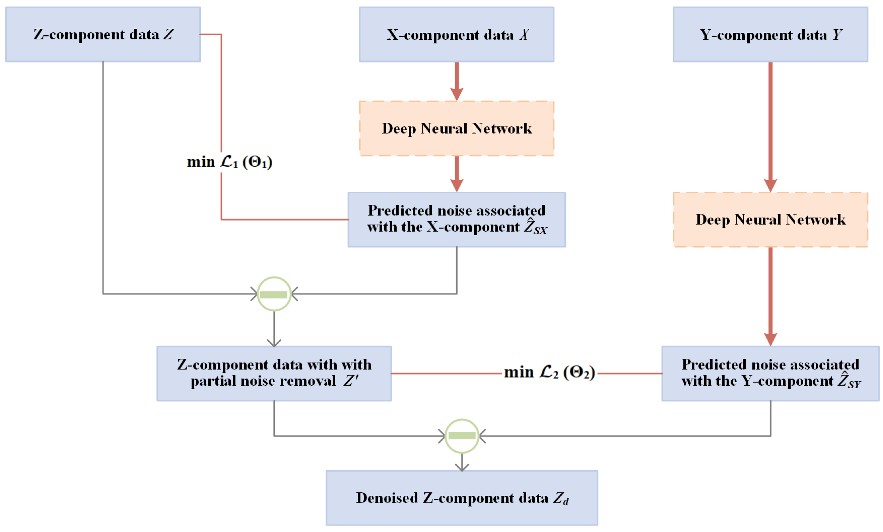
To introduce the mathematical model of the proposed method, we define as the output of a neural network with weights on input •. Figure 1 shows the workflow of the proposed method, and the structure of the deep neural network is presented in Section 2.2. Since the shear wave noise in the Z-component data is related to the two horizontal components (X- and Y-component), we take the X- and Y-component as noise models in two successive steps to remove the noise related to the X-component (denoted by ) and the noise related to the Y-component (denoted by ), respectively.
First, the X-component data () are input into the neural network as a noise model with the following loss function (seen in Equation (5)).
In this way, the output of the network is expected to be the predicted noise associated with the X-component after training, which is essentially an estimate of the true noise with respect to the X-component (symbolized by ) in Z-component data. Subtracting from yields the updated Z-component data with leaked X-component noise removed (seen in Equation (6)).
Naturally, in the second step, will be further denoised as the updated noisy data by repeating the above steps using Y-component data () as the reference noise model. After feeding into the network and optimizing the network parameters with Equation (7) as the loss function, the final denoised Z-component () can be reconstructed as follows:
In this case, the minimization of the loss function (Equations (5) and (7)) corresponds to the minimization of the objective function (Equation (4)) in the traditional method, while the network parameters correspond to the leakage coefficients (). Moreover, DNNs can learn nonlinear mapping relationships, in contrast to the linear iterations of traditional adaptive subtraction, to better represent the complex relationships of data.
2.2. Network Architecture
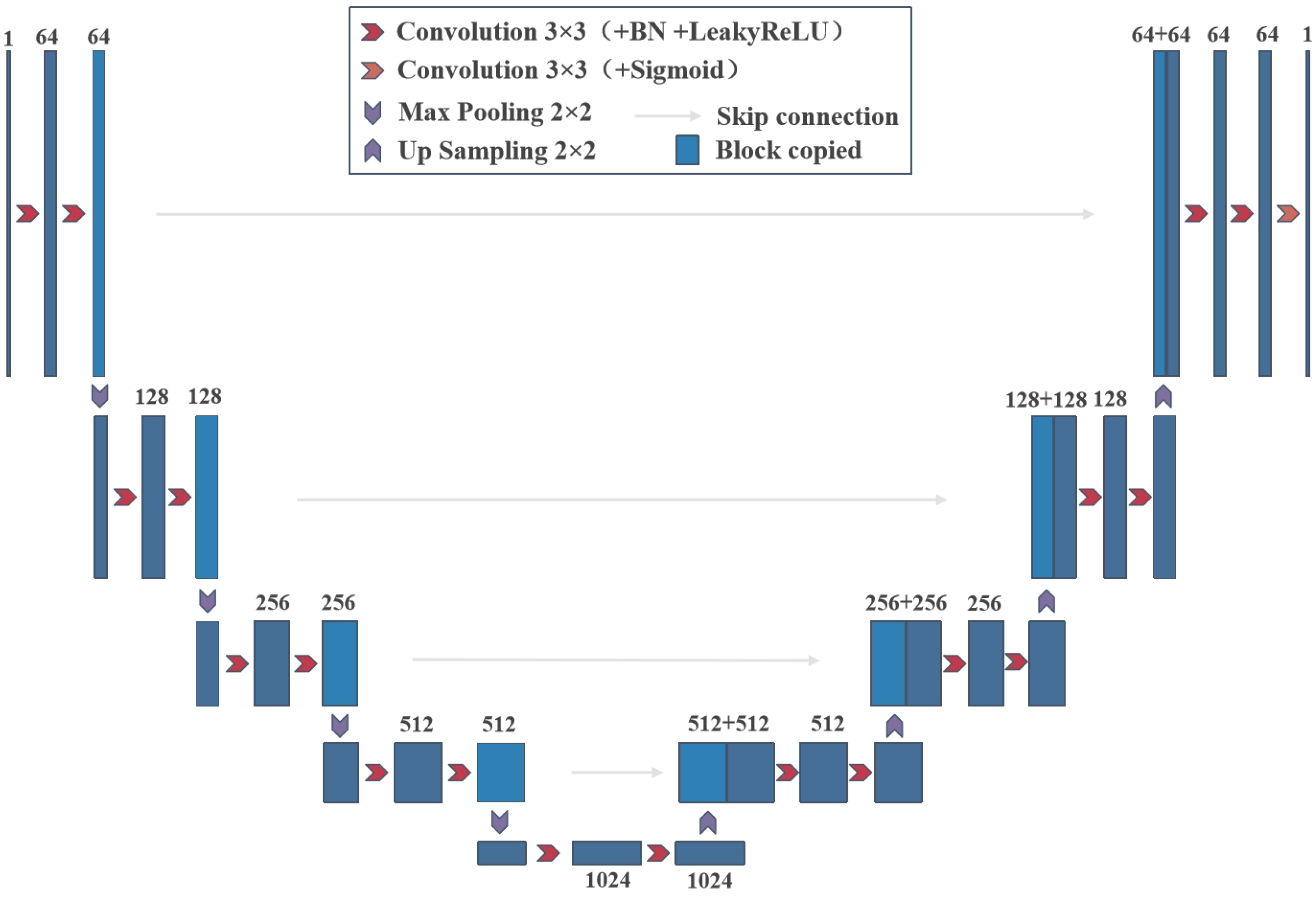
The network we used is based on U-Net. U-Net is a fully convolutional network, first proposed by Ronneberger et al. [41], and widely used in various domains due to its outstanding generalization ability. The U-Net is composed of two parts: the contracting path, known as the encoder, is used for extracting features and context information; and a symmetric expanding path responsible for resolution restoration, which can be understood as a decoder. The features extracted by the encoder are incorporated together with the feature maps in the decoder through skip connections. Compared to the standard convolution neural network (CNN), U-Net uses skip connections so that the low- and high-level features of the input data do not decay inside network propagation. These architecture choices collectively contribute to the effectiveness of the U-Net. The structure of the U-Net network used in this paper is shown in Figure 2.
The input to the network is the reference noise (X- or Y-component data), and the output is expected to be real noise. The encoder on the left consists of four blocks, each containing two convolutional layers and a maximum pooling layer for downsampling, with a total of four downsamplings. After one downsample operator, the number of feature channels is doubled, and the length and width of the feature map halved. The decoder on the right contains four blocks consisting of two convolutional layers, a upsampling layer and a splicing of the feature maps from the corresponding decoder. The last layer of the decoder is a convolutional layer. The size of the convolution kernels of all layers is 3 × 3, and the number of feature channels in each convolutional computation is shown in Figure 2. Except for the last layer, batch normalization (BN) is applied after each convolutional layer to mitigate over-fitting and reduce the training time [42], and the LeakyReLU activation function [43] is used to enhance the nonlinearity.
3. Experiments
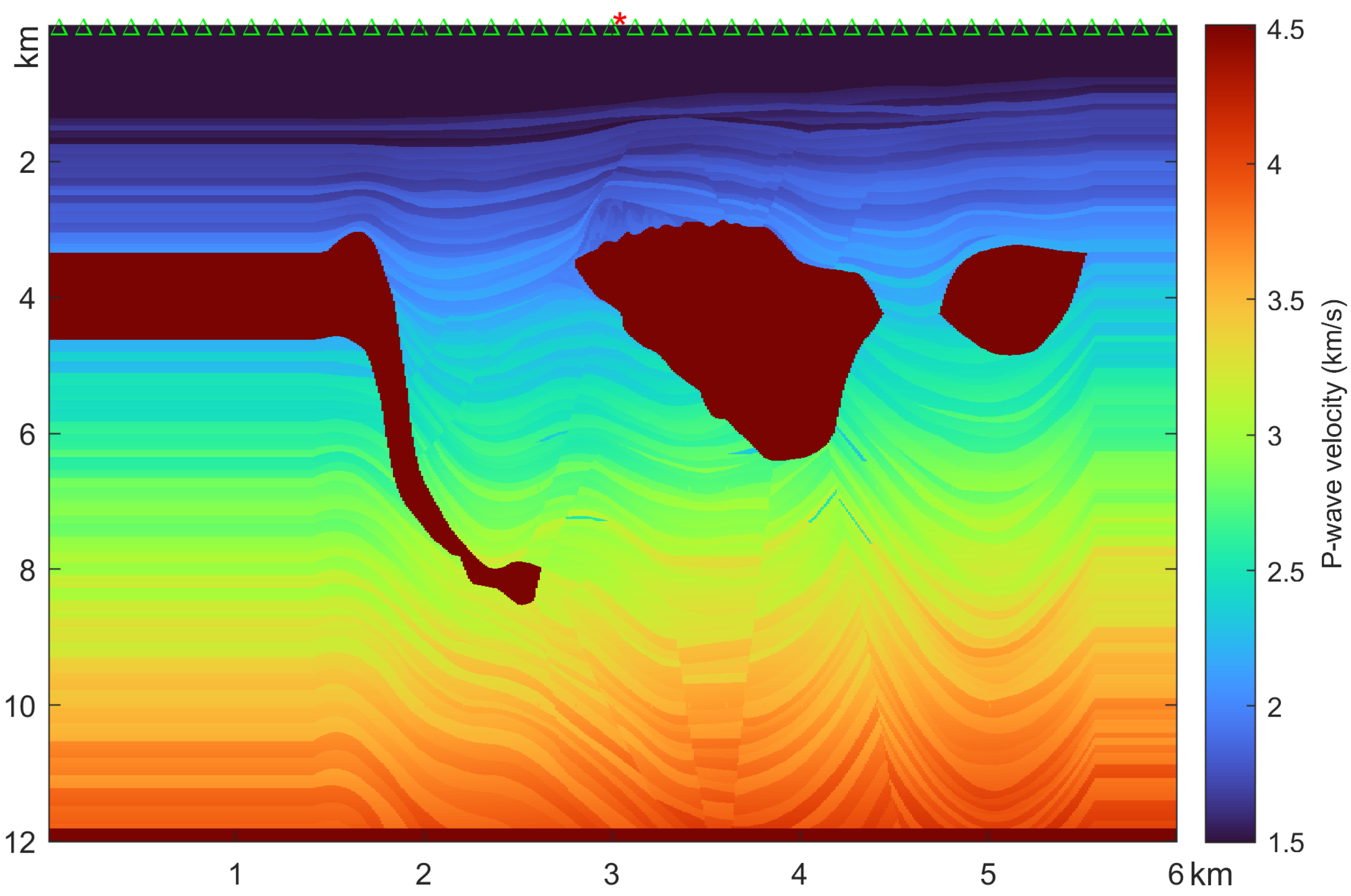
In this section, we apply the proposed method on one set of synthetic data and one field data for numerical experiments to verify the effectiveness of our method. The set of synthetic data is obtained by forward modeling on the Pluto model (Figure 3) to obtain clean P-wave signal data, and a total of 94 receivers and one seismic source are deployed with a recording time of 7 s and a sampling interval of 2 ms. The P-wave signal data are regarded as clean Z-component data. Then, we add horizontal component data (Figure 4b,c) from the field data in various proportions to obtain a set of noisy Z-component data. Such an approach mimics the actual situation where noise behaves as coherent noise in CRG, and the proportions and experimental details are described in Section 3.1. Field OBN data used in this paper were collected in offshore China. We select part of the data from one of the CRGs for testing. Each component of the geophone data contains 94 traces of seismic data, and there are 3501 time samples with a time interval of 2 ms in each trace. The size of synthetic data and field data for experiments are both 3501 × 94. Before feeding the data into the network, we pad zeros around the data according to the structure of the U-Net (Figure 2) to ensure that the size of the data remains consistent after the convolution operation and then normalize the data between 0 and 1. The processed data are input into the network for training, utilizing the Adam optimization algorithm. In addition, all experiments are implemented on the Pytorch 1.10.2 framework with CPU and GPU calculations.
3.1. Synthetic Example
Figure 4a shows the synthetic seismic data obtained from the Pluto velocity model, denoted as . Figure 4b,c show the X- and Y-component from the field data, denoted as and , respectively. For a clear display, the amplitude of the X- and Y-component are magnified by two times. Due to the complexity of the causes of shear wave leakage, it is difficult to model leaking weighting coefficients that are sufficiently approximate to the actual situation. We add and to the clean P-wave data () in a fixed ratio and perform numerical experiments in the simplified case. The synthetic noisy Z-component data (denoted as ) are obtained through Equation (9), where represents the proportion of added noise. We set to 0.5, 1, and 2, respectively, then generate three clean and noisy data pairs (denoted as Dataset 1-1, 1-2 and 1-3) for experiments. In the network training, the learning rate is set at 0.001, the batch size is fixed to 1, and the number of iterations is 500. The network hyperparameters are selected by trial and error.
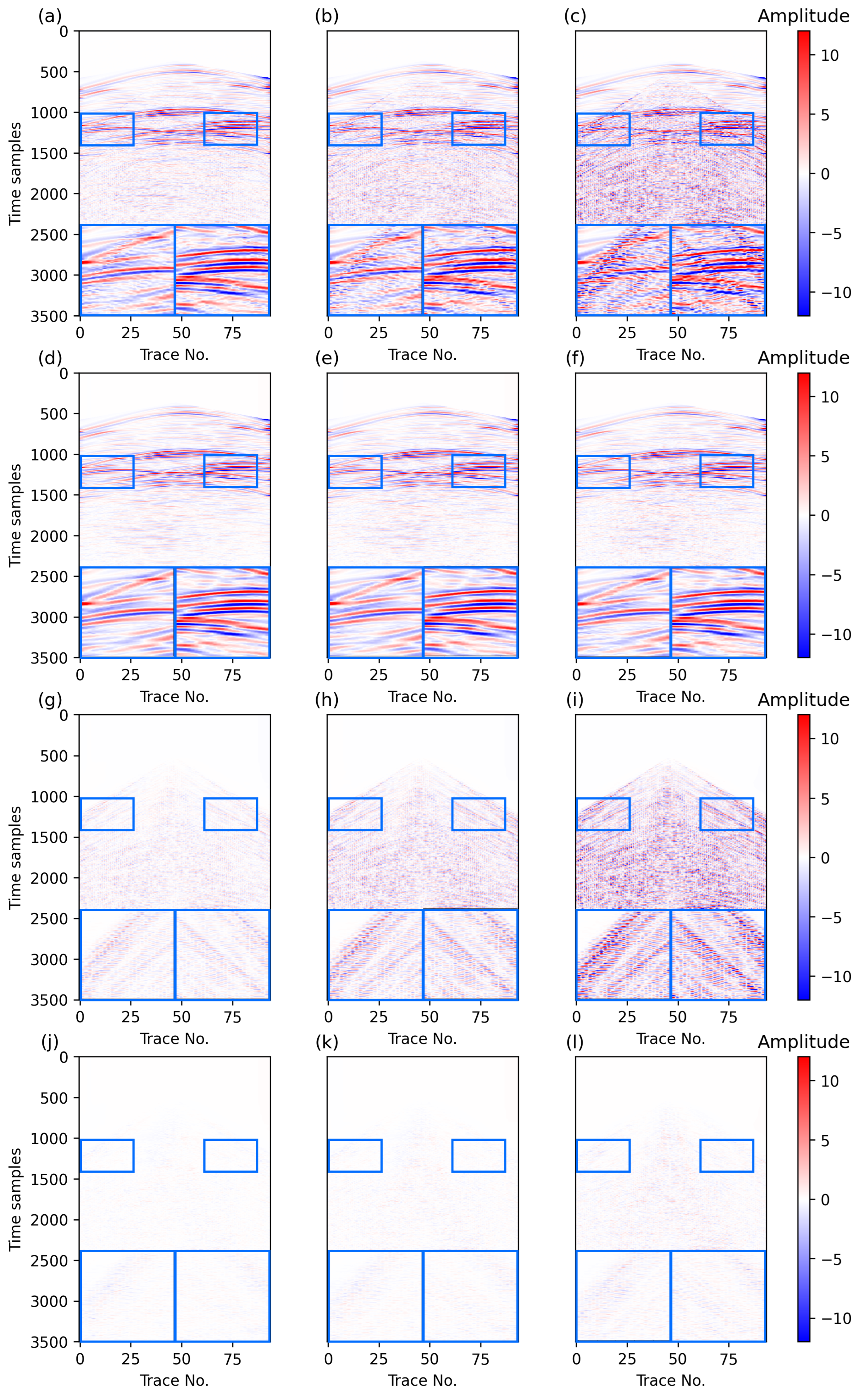
The noisy data (Figure 5a–c) in the synthetic dataset show a large amount of noise with different amplitudes, and in many regions, the noise overlaps the valid signal, such as the blue rectangles area. The second row of Figure 5 displays the denoising results of applying the proposed method, and the predicted noise and the error of the denoising result with respect to the clean data are shown in the third and last rows in Figure 5, respectively. In the denoising results (Figure 5d–f), it can be seen that the large amount of shear noise shown in the noisy data has been eliminated. The similarity of the denoising results to the clean data (Figure 4a) demonstrates the effectiveness of the denoising method. The error graphs (Figure 5j–l) show that there is only a weak residue of noise in the denoising results. Moreover, no significant signal leakage is observed in the predicted noise and error diagrams. To better analyze the results, we give the magnified display results of the two blue rectangles. It can be seen that most of the noise is removed in the noise–signal overlap region, and there is little damage to the signal. The above results indicate that the method in this paper can achieve both signal protection and noise removal, and it is still effective in the signal–noise overlap region.
Additionally, we report the signal-to-noise ratio (SNR) as a quantitative metric to analyze the denoising results. The SNR is calculated as follows:
where S is the clean signal and represents the reconstructed data. As we know, a higher SNR means a better quality of data. After denoising, the SNRs of noisy data from Dataset 1-1, 1-2 and 1-3 are improved from 6.55 dB, 0.53 dB, −5.49 dB to 16.12 dB, 13.47 dB, 9.47 dB, respectively, indicating the effectiveness of the proposed method. Table 1 shows the SNRs of the data before and after denoising.
3.2. Field Example
Figure 6a shows the raw hydrophone component data, and Figure 6b shows the raw Z-component data. It can be seen that the Z-component has a lower signal-to-noise ratio compared to the P-component data, which affects subsequent data processing and interpretation. The original horizontal X- and Y-component in the field data are shown in Figure 4, which are pre-processed and then sequentially fed into the network to predict the noise in the noisy Z-component (Figure 6b). The similarity between the shear wave noise in the Z-component and two horizontal component data suggests that it is reasonable to use the X- and Y-component data as the initial noise model. In the network training, the learning rate is set to 0.001, the batch size is fixed to 1, and the number of iterations is 1900. The network hyperparameters are selected by trial and error.
To analyze the denoising results, we plot the original Z-component data and the denoising results by applying the proposed deep learning method for shear wave noise attenuation in Figure 7. Black arrows point out much obvious noise, and red arrows indicate signals. Figure 7b,c show the denoising results and predicted noise by the proposed method. The blue rectangle of the noisy Z-component is where the noise amplitudes are large. The noise overlaps the signal and even masks the valid signal. The proposed method in this paper effectively suppresses the shear wave noise. The magnified display results of the data corresponding to the blue rectangles in Figure 7 are shown in Figure 8. The black and red circles indicate the area where the noise and signal overlap. Our method exhibits effective denoising in these region. Particularly, the red circles highlight that our method achieves signal recovery while denoising. In addition, the continuity of the valid signal is improved.
For field data, we cannot use SNR as a metric for evaluating the denoising results due to the unavailability of clean data. Inspired by Jeong and Tsingas [19], we utilize the raw P-component data as a reference to evaluate the denoising results since the pressure wave recorded by a hydrophone is not disturbed by shear wave noise. Figure 9a shows the auto-correlation of P-component data used as a reference. Figure 9b shows a cross-correlation plot between the P-component and the raw Z-component, and Figure 9c shows a cross-correlation plot between the P-component and the denoised Z-component. Compared with Figure 9b, Figure 9c has a higher similarity with Figure 9a, which indicates that the proposed method effectively suppresses the shear noise while retaining the desired signal.
Furthermore, we estimate the local slope using the dip2d function in the Pyseistr package [44] to analyze the denoising effect. Figure 10a shows the estimated local slope of the P-component data which are considered as the reference indicating denosing performance. Figure 10b shows the estimated local slope of the raw Z-component data, and Figure 10c shows the result obtained by the proposed denoising method, which better matches the reference. The second row of Figure 10 shows the estimated local slope at time sampling points 500–1500 in the first row, showing more clearly the similarity between Figure 10c and Figure 10a. These results indicate that the proposed method in this paper can remove the shear wave noise with protection of the signal, which verifies the effectiveness of the method.
4. Discussions
4.1. Order of Denoising
Since the shear noise in the Z-component is related to both of the two horizontal components, we need to consider a different denoising order. First, we do not consider the case of removing the noise related to both components simultaneously, as this would make it difficult for the network to distinguish the features of the noise and the signal. After removing one first, the SNR of the data is improved and the features of the other are more easily recognized by the network. Different from the previous operation of removing X- and Y-component leakage successively, we consider the case where the noise related to the Y-component is removed first in step one and then the noise of the X-component in the second step.
Table 2 shows the denoising results and SNRs before and after denoising on the synthetic Dataset 1-1, 1-2 and 1-3 by first removing the noise related to the Y-component and then removing the noise related to the X-component. The network training parameters are the same as those in Section 3.1 for comparison. Combined with Table 1, it can be seen that both denoising orders improve the SNRs of the original data, with little difference in the magnitude of the improvement.
Considering that the X- and Y-components of the field data may leak noise in different proportions, we generated a second set of clean–noisy data pairs in the manner of Equation (11).
We generate a total of six clean–noisy data pairs by setting different combinations of values for and and then perform numerical experiments under two denoising orders. The network parameters are all set with reference to Section 3.1. The SNRs before and after denoising are shown in Table 3. Denoising order I means that the noise associated with the X-component is removed first, followed by the noise associated with the Y-component, and order II is reversed. These results show that both denoising orders improve the SNRs of the data in various scenarios. Additionally, the proportion of noise leakage associated with each component is stronger, achieving better denoising results by removing the noise first. At the same time, this is also related to the energy strength of the two horizontal components themselves. Overall, removing the component that leaks stronger noise first can achieve better denoising results. For the field data, we cannot know the proportion of noise leakage. By comparing the data, we can roughly see that the energy of the noise related to X-component is slightly stronger than that of the Y-component (seen in Figure 11). Therefore, for field OBN data, we choose to remove the noise related to the X-component first and then remove the noise related to the Y-component.
4.2. Hyperparameters
The settings of the hyperparameters affect the performance of the network, with inappropriate settings potentially leading to the over-fitting or under-fitting of the model. Network parameter regularization also has the effect of avoiding over-fitting. It is important to note that, in our context, over-fitting refers to the presence of some signals in the noise predicted by the network, resulting in signal damage in the output. Conversely, under-fitting means that the true noise was not adequately predicted, leaving some noise in the result. In this section, we conduct experiments when removing the noise related to the X-component (step one) for synthetic data to examine the impact of the learning rate and network parameter regularization. The initial learning rate is set to 0.001, and the coefficient for network parameter regularization is set to 0. We then vary the parameter values for testing.
Figure 12 demonstrates the changes in the loss function values and corresponding SNRs for network training at a learning rate of 0.001. Figure 13 depicts the variations in the loss function values and SNRs for network training at a learning rate of 0.01 and 0.0001, respectively. With a learning rate of 0.01, the model exhibits over-fitting after approximately 50 iterations, causing the loss function to oscillate widely and rendering the model unstable. When the learning rate is 0.0001, the SNR increases very little as the values of loss function decrease, indicating under-fitting. Therefore, setting the learning rate to 0.001 gives more reasonable results. Furthermore, using network parameter regularization brings no significant improvement to the denoising effect in our tests (seen in Figure 14). Consequently, we choose a learning rate of 0.001 without network parameter regularization as the optimal configuration during network training.
4.3. Limitation and Future Work
The proposed method in this paper does not require clean data. The network learns the features of the noise from the noise model and makes predictions, essentially employing self-supervised learning. However, this does not mean that our method is fully automatic. It is necessary to adjust the network parameters accordingly to different data features due to the complexity of field data. In addition, the time cost on network training is insufficient for industrial applications. Therefore, future work will focus on improving the efficiency. Meanwhile, different DNN structures to replace U-Net to further improve the results can be considered. Combinations with filter-based methods can also be investigated.
5. Conclusions
In this paper, we provide a new solution to attenuate the shear wave noise in OBN data. Our method leverages self-supervised deep learning to perform an adaptive subtraction of shear wave noise. Compared with traditional adaptive subtraction, this method utilizes the rich information within the data and the powerful nonlinear fitting capability of DNN. Experiments on synthetic data verify the feasibility and effectiveness of the method. Simultaneously, the application on field data demonstrates that the proposed method effectively removes the shear wave noise while protecting the signal. We also conducted a comprehensive investigation of the denoising order and parameter settings of our method, providing insights into their influence on the denoising results. In conclusion, the proposed method can effectively remove the shear wave noise in the Z-component while preserving the signal, showing potential applications in the processing of data for OBN acquisition.
Author Contributions
Conceptualization, L.C., Z.C. and B.W.; methodology, L.C., Z.C. and B.W.; investigation, L.C. and Z.C.; formal analysis, L.C.; data curation, L.C. and Z.C.; visualization, L.C.; supervision, B.W. and J.G.; funding acquisition, B.W.; writing—original draft, L.C. All authors have read and agreed to the published version of the manuscript.
Funding
This work was supported by the Natural Science Basic Research Program of Shaanxi under Program 2023-JC-YB-269.
Institutional Review Board Statement
Not applicable.
Informed Consent Statement
Not applicable.
Data Availability Statement
The raw data supporting the conclusions of this article will be made available by the authors on request.
Conflicts of Interest
The authors declare no conflicts of interest.
Abbreviations
The following abbreviations are used in this manuscript:
| OBN | Ocean Bottom Node |
| TS | Towed Streamer |
| OBS | Ocean Bottom Seismometer |
| OBC | Ocean Bottom Cable |
| CSG | common shot gathers |
| CRG | common receiver gathers |
| DNN | deep neural network |
| ANN | artificial neural network |
| GAN | generative adversarial network |
| CNN | convolutional neural network |
| CGLS | conjugate gradient least squares |
| IRLS | iterative reweighted least squares |
| BN | batch normalization |
| Leaky ReLU | leaky rectified linear unit |
| SNR | signal-to-noise ratio |
References
- Zhang, D.; Tsingas, C.; Ghamdi, A.A.; Huang, M.; Jeong, W.; Sliz, K.K.; Aldeghaither, S.M.; Zahrani, S.A. A Review of OBN Processing: Challenges and Solutions. J. Geophys. Eng. 2021, 18, 492–502. [Google Scholar] [CrossRef]
- Yu, J.; Kim, B.Y.; Joo, Y. A Processing for Ocean-Bottom Multicomponent Data with Seismic Interferometry: A Case Study of Southern Offshore in Korea. Explor. Geophys. 2023, 54, 533–543. [Google Scholar] [CrossRef]
- Dankbaar, J.W.M. Separation of P- and S-Waves. Geophys. Prospect. 1985, 33, 970–986. [Google Scholar] [CrossRef]
- Yu, Z.; Kumar, C.; Ahmed, I. Ocean Bottom Seismic Noise Attenuation Using Local Attribute Matching Filter. In Proceedings of the SEG Technical Program Expanded Abstracts, San Antonio, TX, USA, 18–23 September 2011; Society of Exploration Geophysicists: Houston, TX, USA, 2011; pp. 3586–3590. [Google Scholar] [CrossRef]
- Bouchaala, F.; Ali, M.Y.; Matsushima, J.; Bouzidi, Y.; Jouini, M.S.; Takougang, E.M.; Mohamed, A.A. Estimation of seismic wave attenuation from 3D seismic data: A case study of OBC data acquired in an offshore oilfield. Energies 2022, 15, 534. [Google Scholar] [CrossRef]
- Basu, S.; Mohapatra, S.; Viswanathan, S. Pre-conditioning of data before PZ summation in OBC survey—A case study. In Proceedings of the 9th Bennial International Conference & Exposition on Petroleum Geophysics, Hyderabad, India, 16–18 February 2012; pp. 357–362. [Google Scholar]
- Yang, C.; Huang, Y.; Liu, Z.; Sheng, J.; Camarda, E. Shear wave noise attenuation and wavefield separation in curvelet domain. In Proceedings of the SEG International Exposition and Annual Meeting, Online, 11–16 October 2020; SEG: Houston, TX, USA, 2020; p. D031S032R006. [Google Scholar]
- Paffenholz, J.; Shurtleff, R.; Hays, D.; Docherty, P. Shear Wave Noise on OBS Vz Data-Part I Evidence from Field Data. In Proceedings of the 68th EAGE Conference and Exhibition incorporating SPE EUROPEC, Vienna, Austria, 12–15 June 2006; European Association of Geoscientists & Engineers: Utrecht, The Netherlands, 2006; p. cp-2. [Google Scholar]
- Paffenholz, J.; Docherty, P.; Shurtleff, R.; Hays, D. Shear Wave Noise on OBS Vz Data-Part II Elastic Modeling of Scatterers in the Seabed. In Proceedings of the 68th EAGE Conference and Exhibition incorporating SPE EUROPEC, Vienna, Austria, 12–15 June 2006; European Association of Geoscientists & Engineers: Utrecht, The Netherlands, 2006; p. cp-2. [Google Scholar]
- Yu, S.; Ma, J.; Wang, W. Deep Learning for Denoising. Geophysics 2019, 84, V333–V350. [Google Scholar] [CrossRef]
- Shatilo, A.; Duren, R.; Rape, T. Effect of noise suppression on quality of 2C OBC image. In SEG Technical Program Expanded Abstracts 2004; Society of Exploration Geophysicists: Houston, TX, USA, 2004; pp. 917–920. [Google Scholar]
- Craft, K.L. Geophone noise attenuation and wave-field separation using a multi-dimensional decomposition technique. In Proceedings of the 70th EAGE Conference and Exhibition incorporating SPE EUROPEC, Rome, Italy, 9–12 June 2008; European Association of Geoscientists & Engineers: Utrecht, The Netherlands, 2008; p. cp-40. [Google Scholar]
- Wang, Y.; Wang, R. S-wave suppression in the vertical component of 4-C OBC data. In Proceedings of the SEG International Exposition and Annual Meeting, Houston, TX, USA, 24–29 September 2017; SEG: Houston, TX, USA, 2017; p. SEG-2017. [Google Scholar]
- Verschuur, D.J.; Berkhout, A.; Wapenaar, C. Adaptive surface-related multiple elimination. Geophysics 1992, 57, 1166–1177. [Google Scholar] [CrossRef]
- Verschuur, D.; Berkhout, A. Estimation of multiple scattering by iterative inversion, Part II: Practical aspects and examples. Geophysics 1997, 62, 1596–1611. [Google Scholar] [CrossRef]
- Guitton, A.; Verschuur, D. Adaptive subtraction of multiples using the L1-norm. Geophys. Prospect. 2004, 52, 27–38. [Google Scholar] [CrossRef]
- Hlebnikov, V.; Elboth, T.; Vinje, V.; Gelius, L.J. Noise types and their attenuation in towed marine seismic: A tutorial. Geophysics 2021, 86, W1–W19. [Google Scholar] [CrossRef]
- Fomel, S. Adaptive multiple subtraction using regularized nonstationary regression. Geophysics 2009, 74, V25–V33. [Google Scholar] [CrossRef]
- Jeong, W.; Tsingas, C. A de-noising methodology for multi-component seafloor nodal geophones. In Proceedings of the 81st EAGE Conference and Exhibition, London, UK, 3–6 June 2019; European Association of Geoscientists & Engineers: Utrecht, The Netherlands, 2019; Volume 2019, pp. 1–5. [Google Scholar]
- Wang, S.; Song, P.; Tan, J.; He, B.; Xia, D.; Wang, Q.; Du, G. Deep learning-based attenuation for shear-wave leakage from ocean-bottom node data. Geophysics 2023, 88, V127–V137. [Google Scholar] [CrossRef]
- Zhang, K.; Zuo, W.; Chen, Y.; Meng, D.; Zhang, L. Beyond a Gaussian Denoiser: Residual Learning of Deep CNN for Image Denoising. IEEE Trans. Image Process. 2017, 26, 3142–3155. [Google Scholar] [CrossRef] [PubMed]
- Lempitsky, V.; Vedaldi, A.; Ulyanov, D. Deep Image Prior. In Proceedings of the 2018 IEEE/CVF Conference on Computer Vision and Pattern Recognition, Salt Lake City, UT, USA, 18–22 June 2018; pp. 9446–9454. [Google Scholar] [CrossRef]
- Mousavi, S.M.; Beroza, G.C. Deep-Learning Seismology. Science 2022, 377, eabm4470. [Google Scholar] [CrossRef] [PubMed]
- Mousavi, S.M.; Beroza, G.C.; Mukerji, T.; Rasht-Behesht, M. Applications of Deep Neural Networks in Exploration Seismology: A Technical Survey. Geophysics 2024, 89, WA95–WA115. [Google Scholar] [CrossRef]
- Adler, A.; Araya-Polo, M.; Poggio, T. Deep Learning for Seismic Inverse Problems: Toward the Acceleration of Geophysical Analysis Workflows. IEEE Signal Process. Mag. 2021, 38, 89–119. [Google Scholar] [CrossRef]
- Li, Y.; Song, J.; Lu, W.; Monkam, P.; Ao, Y. Multitask Learning for Super-Resolution of Seismic Velocity Model. IEEE Trans. Geosci. Remote Sens. 2021, 59, 8022–8033. [Google Scholar] [CrossRef]
- Yuan, S.; Liu, J.; Wang, S.; Wang, T.; Shi, P. Seismic Waveform Classification and First-Break Picking Using Convolution Neural Networks. IEEE Geosci. Remote Sens. Lett. 2018, 15, 272–276. [Google Scholar] [CrossRef]
- Wang, B.; Zhang, N.; Lu, W.; Wang, J. Deep-learning-based seismic data interpolation: A preliminary result. Geophysics 2019, 84, V11–V20. [Google Scholar] [CrossRef]
- Liu, X.; Wu, B.; Yang, H. Multi-Task Full Attention U-Net for Prestack Seismic Inversion. IEEE Geosci. Remote Sens. Lett. 2023, 20, 3002605. [Google Scholar] [CrossRef]
- Zhang, S.B.; Si, H.J.; Wu, X.M.; Yan, S.S. A comparison of deep learning methods for seismic impedance inversion. Pet. Sci. 2022, 19, 1019–1030. [Google Scholar] [CrossRef]
- Wu, X.; Liang, L.; Shi, Y.; Fomel, S. FaultSeg3D: Using Synthetic Data Sets to Train an End-to-End Convolutional Neural Network for 3D Seismic Fault Segmentation. Geophysics 2019, 84, IM35–IM45. [Google Scholar] [CrossRef]
- Wang, L.; Wang, Z.; Wang, J.; Liu, P. A Survey of Random Noise Suppression Methods for Seismic Data based on Deep Learning. In Proceedings of the 2022 2nd International Conference on Networking, Communications and Information Technology (NetCIT), Manchester, UK, 26–27 December 2022; pp. 572–576. [Google Scholar] [CrossRef]
- Zhang, M.; Liu, Y.; Bai, M.; Chen, Y. Seismic Noise Attenuation Using Unsupervised Sparse Feature Learning. IEEE Trans. Geosci. Remote Sens. 2019, 57, 9709–9723. [Google Scholar] [CrossRef]
- Qiu, C.; Wu, B.; Liu, N.; Zhu, X.; Ren, H. Deep Learning Prior Model for Unsupervised Seismic Data Random Noise Attenuation. IEEE Geosci. Remote Sens. Lett. 2022, 19, 7502005. [Google Scholar] [CrossRef]
- Xu, Z.; Luo, Y.; Wu, B.; Meng, D. S2S-WTV: Seismic Data Noise Attenuation Using Weighted Total Variation Regularized Self-Supervised Learning. IEEE Trans. Geosci. Remote Sens. 2023, 61, 5908315. [Google Scholar] [CrossRef]
- Wang, K.; Hu, T.; Wang, S.; Wei, J. Seismic Multiple Suppression Based on a Deep Neural Network Method for Marine Data. Geophysics 2022, 87, V341–V365. [Google Scholar] [CrossRef]
- Yuan, Y.; Si, X.; Zheng, Y. Ground-Roll Attenuation Using Generative Adversarial Networks. Geophysics 2020, 85, WA255–WA267. [Google Scholar] [CrossRef]
- Wang, K.; Hu, T.; Zhao, B.; Wang, S. Surface-Related Multiple Attenuation Based on Self-Supervised Deep Neural Network with Local Wavefield Characteristics. Geophysics 2023, 88, V387–V402. [Google Scholar] [CrossRef]
- Li, Z.; Sun, N.; Gao, H.; Qin, N.; Li, Z. Adaptive Subtraction Based on U-Net for Removing Seismic Multiples. IEEE Trans. Geosci. Remote Sens. 2021, 59, 9796–9812. [Google Scholar] [CrossRef]
- Liu, L.; Hu, T.; Huang, J.; Wang, S. Adaptive Surface-Related Multiple Subtraction Based on Convolutional Neural Network. IEEE Geosci. Remote Sens. Lett. 2022, 19, 8021905. [Google Scholar] [CrossRef]
- Ronneberger, O.; Fischer, P.; Brox, T. U-Net: Convolutional Networks for Biomedical Image Segmentation. In Medical Image Computing and Computer-Assisted Intervention – MICCAI 2015; Navab, N., Hornegger, J., Wells, W.M., Frangi, A.F., Eds.; Springer International Publishing: Cham, Switzerland, 2015; Volume 9351, pp. 234–241. [Google Scholar] [CrossRef]
- Ioffe, S.; Szegedy, C. Batch normalization: Accelerating deep network training by reducing internal covariate shift. In Proceedings of the 32nd International Conference on International Conference on Machine Learning, ICML’15, Lille, France, 6–11 July 2015; JMLR.org: Norfolk, MA, USA, 2015; Volume 37, pp. 448–456. [Google Scholar]
- Maas, A.L.; Hannun, A.Y.; Ng, A.Y. Rectifier nonlinearities improve neural network acoustic models. In Proceedings of the ICML, Atlanta, GA, USA, 17–19 June 2013; Volume 30, p. 3. [Google Scholar]
- Chen, Y.; Savvaidis, A.; Fomel, S.; Chen, Y.; Saad, O.M.; Oboué, Y.A.S.I.; Zhang, Q.; Chen, W. Pyseistr: A Python Package for Structural Denoising and Interpolation of Multichannel Seismic Data. Seismol. Res. Lett. 2023, 94, 1703–1714. [Google Scholar] [CrossRef]
Figure 1.
The workflow of self-supervised shear wave noise adaptive subtraction in OBN data. In the first step, the X-component data are input into the network to predict the noise related to the X-component, then subtract the noise from the noisy Z-component data. In the second step, the Y-component data are input to the network to predict the noise related to the Y-component, and the denoising result is obtained by subtracting the predicted noise.

Figure 2.
The architecture of U-Net used for shear wave attenuation of OBN data.

Figure 3.
Pluto velocity model used for synthetic data generation. The red asterisk represents the location of the source, while the green triangles indicate the position of the receivers.
Figure 3.
Pluto velocity model used for synthetic data generation. The red asterisk represents the location of the source, while the green triangles indicate the position of the receivers.

Figure 4.
Synthetic data and X- and Y-component field data. (a) Synthetic P-wave data (synthetic clean Z-component data). (b) X-component of field OBN data. (c) Y-component of field OBN data.
Figure 4.
Synthetic data and X- and Y-component field data. (a) Synthetic P-wave data (synthetic clean Z-component data). (b) X-component of field OBN data. (c) Y-component of field OBN data.

Figure 5.
Synthetic data example. First row: noisy data of Dataset 1-1 (a), Dataset 1-2 (b) and Dataset 1-3 (c). Second row: noise attenuation results of Dataset 1-1 (d), 1-2 (e) and 1-3 (f). Third row: predicted noise of Dataset 1-1 (g), 1-2 (h) and 1-3 (i). Bottom row: difference between the denoising results and clean data of Dataset 1-1 (j), 1-2 (k) and 1-3 (l) by subtracting Figure 4a from (d–f), respectively. The two blue rectangles above each image are magnified correspondingly in the lower left and lower right of the figure.

Figure 6.
Field OBN data example. (a) Raw P-component data. (b) Raw Z-component data.

Figure 7.
Field data example. (a) Raw Z-component data. (b) Denoising result by the proposed method. (c) Predicted noise by the proposed method. The blue rectangular areas are seismic data from time sampling points 500–1500. Black arrows point out several obvious noise and red arrows indicate signals.

Figure 8.
Magnified display results of the blue rectangular areas in Figure 7. (a) Raw Z-component data. (b) Denoising result by the proposed method. (c) Predicted noise by the proposed method. The black and red circles indicate the area where noise and signal overlap.
Figure 8.
Magnified display results of the blue rectangular areas in Figure 7. (a) Raw Z-component data. (b) Denoising result by the proposed method. (c) Predicted noise by the proposed method. The black and red circles indicate the area where noise and signal overlap.

Figure 9.
Correlation plots of the P-component [Figure 6a] with respect to (a) hydrophone (auto-correlation), (b) raw Z-component [Figure 6b (also Figure 7a)], and (c) denoised Z-component [Figure 7b], respectively.

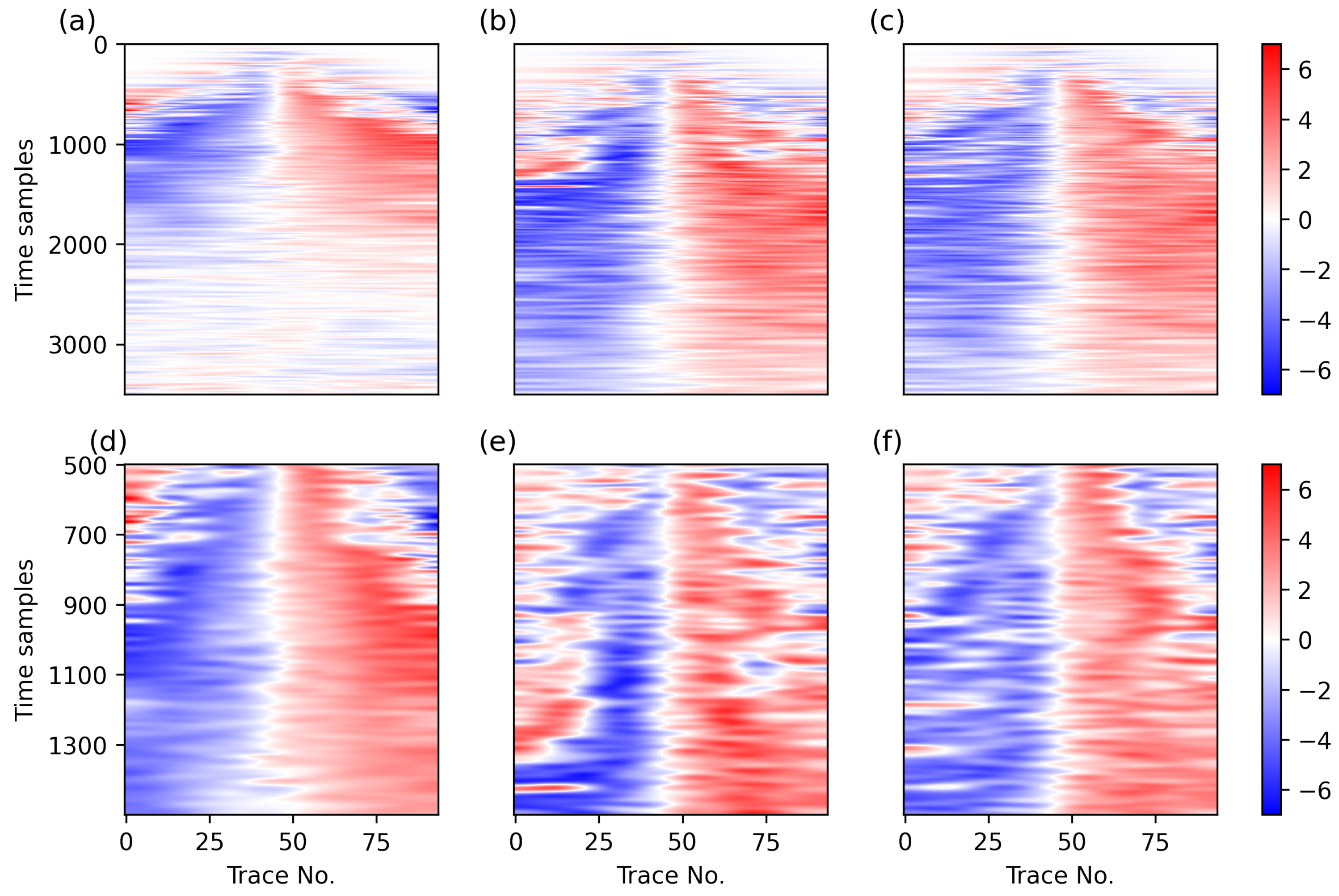
Figure 10.
Local slope estimated from the CRGs of the P-component [Figure 6a] (a) hydrophone, (b) raw Z-component [Figure 6b (also in Figure 7a)] and (c) denoised Z-component [Figure 7b], respectively. The second row (d–f): Magnified display result of the estimated local slope at time sampling points 500–1500 in the first row.

Figure 11.
Comparison of the three components of field OBN data. (a) From left to right, the Y-, Z-, X- and Z-component. (b) From left to right, the Z-, X-, Z- and Y-component.
Figure 11.
Comparison of the three components of field OBN data. (a) From left to right, the Y-, Z-, X- and Z-component. (b) From left to right, the Z-, X-, Z- and Y-component.

Figure 12.
Loss function and SNR curves in network training without network parameter regularization (learning rate = 0.001).
Figure 12.
Loss function and SNR curves in network training without network parameter regularization (learning rate = 0.001).

Figure 13.
Loss function and SNR curves in network training without network parameter regularization. (a) Learning rate = 0.01. (b) Learning rate = 0.0001.
Figure 13.
Loss function and SNR curves in network training without network parameter regularization. (a) Learning rate = 0.01. (b) Learning rate = 0.0001.

Figure 14.
Loss function and SNR curves in network training (learning rate = 0.001). (a) Weight decay = . (b) Weight decay = .
Figure 14.
Loss function and SNR curves in network training (learning rate = 0.001). (a) Weight decay = . (b) Weight decay = .


Table 1.
SNRs of synthetic data examples before and after denoising.
| Dataset 1-1 | Dataset 1-2 | Dataset 1-3 | |
|---|---|---|---|
| Noisy data | 6.55 dB | 0.53 dB | −5.49 dB |
| Denoising result | 16.12 dB | 13.47 dB | 9.47 dB |
Table 2.
SNRs of synthetic data examples before and after denoising for removing Y-component first.
| Dataset 1-1 | Dataset 1-2 | Dataset 1-3 | |
|---|---|---|---|
| Noisy data | 6.55 dB | 0.53 dB | −5.49 dB |
| Denoising result | 16.36 dB | 14.69 dB | 11.14 dB |
Table 3.
SNRs of the second set of synthetic data examples before and after denoising.
| Dataset 2-1 | Dataset 2-2 | Dataset 2-3 | Dataset 2-4 | Dataset 2-5 | Dataset 2-6 | |
|---|---|---|---|---|---|---|
| Noisy data | 3.62 dB | 1.81 dB | −2.40 dB | −4.21 dB | −1.01 dB | −3.77 dB |
| Order I | 15.61 dB | 13.43 dB | 13.13 dB | 8.18 dB | 15.57 dB | 8.17 dB |
| Order II | 14.74 dB | 16.27 dB | 10.76 dB | 13.59 dB | 10.84 dB | 14.83 dB |
Disclaimer/Publisher’s Note: The statements, opinions and data contained in all publications are solely those of the individual author(s) and contributor(s) and not of MDPI and/or the editor(s). MDPI and/or the editor(s) disclaim responsibility for any injury to people or property resulting from any ideas, methods, instructions or products referred to in the content. |
© 2024 by the authors. Licensee MDPI, Basel, Switzerland. This article is an open access article distributed under the terms and conditions of the Creative Commons Attribution (CC BY) license (https://creativecommons.org/licenses/by/4.0/).
Share and Cite
MDPI and ACS Style
Chen, L.; Chen, Z.; Wu, B.; Gao, J. Self-Supervised Shear Wave Noise Adaptive Subtraction in Ocean Bottom Node Data. Appl. Sci. 2024, 14, 3488. https://doi.org/10.3390/app14083488
AMA Style
Chen L, Chen Z, Wu B, Gao J. Self-Supervised Shear Wave Noise Adaptive Subtraction in Ocean Bottom Node Data. Applied Sciences. 2024; 14(8):3488. https://doi.org/10.3390/app14083488
Chicago/Turabian StyleChen, Lin, Zhihao Chen, Bangyu Wu, and Jing Gao. 2024. "Self-Supervised Shear Wave Noise Adaptive Subtraction in Ocean Bottom Node Data" Applied Sciences 14, no. 8: 3488. https://doi.org/10.3390/app14083488
Note that from the first issue of 2016, this journal uses article numbers instead of page numbers. See further details here.