Data-Driven Identification of Crane Dynamics Using Regularized Genetic Programming

Abstract

The meaningful problem of improving crane safety, reliability, and efficiency is extensively studied in the literature and targeted via various model-based control approaches. In recent years, crane data-driven modeling has attracted much attention compared to physics-based models, particularly due to its potential in real-time crane control applications, specifically in model predictive control. This paper proposes grammar-guided genetic programming with sparse regression (G3P-SR) to identify the nonlinear dynamics of an underactuated crane system. G3P-SR uses grammars to bias the search space and produces a fixed number of candidate model terms, while a local search method based on an l₀-regularized regression results in a sparse solution, thereby also reducing model complexity as well as reducing the probability of overfitting. Identification is performed on experimental data obtained from a laboratory-scale overhead crane. The proposed method is compared with multi-gene genetic programming (MGGP), NARX neural network, and Takagi-Sugeno fuzzy (TSF) ARX models in terms of model complexity, prediction accuracy, and sensitivity. The G3P-SR algorithm evolved a model with a maximum mean square error (MSE) of crane velocity and sway prediction of 1.1860 × 10⁻⁴ and 4.8531 × 10⁻⁴, respectively, in simulations for different testing data sets, showing better accuracy than the TSF ARX and MGGP models. Only the NARX neural network model with velocity and sway maximum MSEs of 1.4595 × 10⁻⁴ and 4.8571 × 10⁻⁴ achieves a similar accuracy or an even better one in some testing scenarios, but at the cost of increasing the total number of parameters to be estimated by over 300% and the number of output lags compared to the G3P-SR model. Moreover, the G3P-SR model is proven to be notably less sensitive, exhibiting the least deviation from the nominal trajectory for deviations in the payload mass by approximately a factor of 10.

1. Introduction

Cranes are material-handling machines widely used in the industrial and logistic sectors. Load transportation is often performed by cranes using ropes, cables, or chains that incorporate the unactuated degrees of freedom to the system, making the transportation tasks more challenging in terms of safety and efficiency as the transient and residual swing of a payload suspended on a rope adversely affects the load positioning performances and may present a safety hazard for the personnel working on-site, the surrounding objects, and the transported cargo, as well as the crane’s structure and equipment affected by the dynamic forces caused by the swinging of the payload. The aforementioned problem is extensively studied in the literature and addressed via different modeling approaches and various anti-sway open-loop and closed-loop control strategies [1,2,3,4]. An accurate dynamic model of a crane system, ensuring the precise prediction of actuated and unactuated states, especially in model-predictive control strategies, is crucial for improving crane operational and energy efficiency, as well as to mitigate the safety hazard. Additionally, the compromise between model performance and complexity is significant for real-time applications, and model structure reduction enhances its interpretability, which is helpful in designing model-based control systems. The accurate prediction of payload positioning is also useful in monitoring applications. In automated crane systems, the monitoring of the position of the load enables one to reduce the risk of collisions with obstructions and restrict motions considering a safety margin and residual sway prediction.

A comprehensive review of various crane dynamic modeling methods and model-based control strategies reported in the literature is presented in [5,6,7]. A majority of the presented approaches are derived from the Euler–Lagrange equation. However, an accurate mathematical model of an underactuated crane dynamic system (e.g., overhead crane, gantry crane, boom crane, tower crane) can be difficult to derive due to the multibody interaction of crane mechanisms and construction elements, cables, hook assembly, load, and other electromechanical components. The dynamic behavior of a crane can be complex, taking into account the variation in payload mass and hoisting rope, nonlinearities and complexities arising from mechanical friction, parameter uncertainty, and possible external disturbances when a crane operates outdoors. Since an accurate model of crane dynamics can be difficult to obtain using analytical methods, machine learning and soft computing techniques are implemented in the identification approaches recently reported in the literature. In terms of controller design, a data-driven approach to develop a model-free controller directly from input–output data is also an interesting alternative (as opposed to a model-based control) that has been successfully applied recently for solving complex dynamic problems [8,9], including the model-independent control of underactuated mechanical systems [10,11].

In [12], Bayesian optimization is used to optimize the crane model and controller with training data collected from experiments carried out on a laboratory-scale overhead crane. A flat output identification algorithm is proposed in [13] to identify a rotary crane based on data measured on a laboratory stand. The idea to approximate the dynamics of a nonlinear underactuated crane system through local linear models is implemented in several papers using Takagi-Sugeno fuzzy (TSF) modeling [14,15,16,17]. An incremental online identification algorithm is proposed to evolve the structure of a TSF model for a laboratory-scale overhead crane [18] and a tower crane [19]. Also, artificial neural network (ANN) models as universal approximators are used to generate black-box nonlinear structures of crane dynamic models and controllers. In recent research works, a double-layer neural network structure has been used to estimate unknown nonlinear parts of ship-mounted crane dynamics [20], a container crane’s dynamics have been approximated using a radial basis function network (RBFN) with Gaussian activation functions [21], and the ANN model has been trained offline using the Bayesian regularization method to predict the parameters of the time-optimal obstacle avoidance trajectory function for a rotary crane [22]. In [23], the adaptive control scheme for a rubber-tired gantry container crane was tested on the laboratory stand, with the ANN models used to estimate the velocities of actuated and underactuated coordinates in three-dimensional spaces, friction parameters, and unknown disturbances. The offline-trained multi-layer perceptron neural network model has been identified to predict the sway of a quay crane’s spreader in [24]. The paper reports the data acquisition equipment and experiments carried out on a physical system and analyses the effectiveness of different learning methods to develop the structure and adjust the weights of the neural network predictor of the spreader’s sway velocity. Different structures of ANN models of an overhead crane’s inverse dynamics were trained and validated using the Levenberg–Marquardt algorithm with data computed in simulations carried out using a model derived analytically [25]. Some works have studied crane modeling and the control problem using metaheuristic algorithms, e.g., genetic algorithm (GA) [26,27]. In [28], an overhead crane’s dynamics were approximated by adaptive neuro-fuzzy inference systems (ANFISs) identified using hairpin RNA GA. A planar crane’s dynamics were decoupled and presented using two ANFIS empirical models of actuated trolley motion and unactuated pendulum motion.

By analyzing the aforementioned works dealing with crane dynamics’ identification, it can be concluded that most of the approaches are based on ANN and TSF models. The majority of works available in the literature focuses on the parameter identification of a predefined model, with only a few works focusing on model structure optimization. Model structure optimization is composed of model term construction and parameter estimation. Model term construction can be formulated as a symbolic regression problem in which a space of mathematical functions is searched to find a set of model terms that minimize a problem-dependent loss function. Genetic programming (GP) is an effective symbolic regression tool to identify both dynamic and static relationships between input–output pairs that can be modeled in a more interpretable form than using the black-box modeling approaches. Multi-dimensional genetic programming (MGP), such as multi-gene genetic programming (MGGP) [29], the feature engineering automation tool (FEAT) [30], and the proposed G3P-SR, naturally tackle both problems simultaneously since each individual is composed of a set of programs whose outputs can then be fed into a deterministic algorithm for parameter estimation. In [31], the MGGP technique was used to establish a dynamic model of an overhead crane. The initial gene weights were estimated using the least squares in the serial-parallel configuration after which the Levenberg–Marquardt algorithm was used to find the local optimum of the simulation error by changing the model to a parallel configuration; however, both the evolutionary process of searching for the best model structure and parameter estimation were guided by the model performance criteria, without taking into account the complexity of the model.

To address this issue, this paper proposes the use of sparse regression on a fixed set of candidate model terms that are obtained from a biased search of the function space. Regularization has been successfully applied in the field of system identification to overcome model complexity and prevent overfitting problems. l₀ regularization is used for promoting sparse solutions, although an l₀-regularized problem is nonconvex and proven to be NP-hard. The most popular regularization methods are based on easier-to-solve, convex relaxations of the l₀ norm such as the l₁ norm, e.g., Lasso or its hybrids introduced in the Elastic Net [32] and Fast Function Extraction (FFX) [33] algorithms.

While most studies incorporate l₁ and l₂ regularization into GP, this paper presents the G3P-SR approach with the l₀ norm for crane dynamic identification. To the best of the authors’ knowledge, the combination of genetic programming and l₀ regularization has been previously adapted only for a static regression problem [34], and other evolutionary sparse regression algorithms are based on a combination of the l₁ and l₂ penalties. An l₀ pseudo-norm penalty is added to the objective function, and the subsequent sparse regression problem is solved by using the monotonically accelerated proximal gradient descent algorithm [35]. The sparse solution reduces the model complexity and decreases the probability of overfitting. The model structure optimization and prediction accuracy over a time-horizon are established as the main goals of identification. G3P-SR is employed to establish an overhead crane dynamic model and predict the sway angle. The proposed method is compared with the NARX-NN and TSF-ARX models, since these approaches are mostly reported in the literature for the data-driven modeling of underactuated crane dynamics. The MGGP method is also included in the comparison since only this method has recently addressed crane dynamics’ identification [31]. A comparative study is performed in terms of the models’ complexity, prediction accuracy, and sensitivity. The experimental data used for identification are obtained from a laboratory overhead crane for different operating conditions. The main contribution of this paper are as follows:

(1)

A data-driven offline identification approach for underactuated crane dynamics is developed using an MGP approach called G3P-SR, which uses grammar-guided genetic programming to bias the search space to produce a fixed set of candidate functions for each individual in the population, while the model term selection as well as their coefficients are obtained via sparse l₀ regression.

(2)

A comparative study is performed with an MGGP, an NARX-NN, and a TSF-ARX model in terms of model complexity, accuracy, uncertainty, and sensitivity.

The rest of this paper is organized as follows. In Section 2, we introduce the proposed G3P-SR method as well as the methods used in our comparison during the identification of the overhead crane’s dynamics, namely, the MGGP, NARX-NN, and linear parameter-varying TSF-ARX models. Section 3 presents the experimental setup of the laboratory overhead crane and provides a discussion of the identification results, including a sensitivity and uncertainty analysis, while the final remarks are made in Section 4.

2. Materials and Methods

Genetic programming has been applied successfully in several difficult problems such as symbolic regression, pattern recognition, and automatic design. A survey and taxonomy of existing GP-based methods can be found in [36]. Symbolic regression seeks to identify a mathematical expression over a space of searchable functions that best fits a data set of input–output pairs $T{=\left\{\left({\mathit{x}}_i,y_i\right)\right\}}_{i=1}^N$ with inputs ${\mathit{x}}_i\in {\mathbb{R}}^n$ and an output variable $y\in \mathbb{R}$. In the G3P–SR algorithm proposed in this paper, an individual ${\varphi }^{P_i}$ in a population $P$ is composed of $q$ transformations (represented by trees), which, in the context of identification, we shall call model terms, of the input $\mathit{x}$ so that ${\varphi }^{P_i}\left(\mathit{x}\right) :{\mathbb{R}}^n\to {\mathbb{R}}^q$

$${\varphi }^{P_i}=\left[\begin{array}{cccc}{\varphi }_1^{P_i}& {\varphi }_2^{P_i}& \dots & {\varphi }_q^{P_i}\end{array}\right]$$

where ${\varphi }_j^{P_i}$ are the semantics of tree $j$ in individual $P_i,$ and the output ${\widehat{y}}^{P_i}$ is a linear combination of the columns of ${\varphi }^{P_i}$ as follows:

$$\widehat{y}=\sum _{j=1}^q{\theta }_j{\varphi }_j$$

(1)

In order to avoid redundant model terms, duplicate model terms are eliminated from the individual, and the search space is constrained by implementing a set of production rules that prevent the model terms in ${\varphi }^{P_i}$ from being composed of linear combinations of other model terms in the same individual. This can be achieved by allowing the addition or subtraction operator to only be used inside a nonlinear function, e.g., the model term ${\varphi }_j^{P_i}=(x_1+x_2)$ is not allowed, as it could be composed as a linear combination of two model terms ${\varphi }_{j+1}^{P_i}=x_1$ and ${\varphi }_{j+2}^{P_i}=x_2$, but the model term ${\varphi }_j^{P_i}=\tanh (x_1+x_2)$ is allowed. The coefficients ${\theta }_j$ of the model terms are found using a deterministic numerical optimization algorithm that usually results in increased accuracy as opposed to traditional genetic programming. Every individual in the population has a fixed number of model terms q, which is a hyperparameter of the G3P-SR algorithm. The library of model terms is assumed to be redundant and only a subset of the model terms in the library is required to model the output y. The model term selection and parameter optimization are performed simultaneously using sparse regression by adding an $l_0$ pseudo-norm penalty. This reduces both the model complexity and the chances of overfitting while training on set T. The sparse solution of (1) means that there are model terms in the individual ${\varphi }^{P_i}$ that have no effect on the model output $\widehat{y}$; however, these model terms, called introns, produce different offsprings when subject to genetic operators.

Several approaches to the input–output modeling of nonlinear dynamical systems have been developed, including the nonlinear autoregressive moving average model with exogenous input (NARMAX) model structure that was introduced in the early 1980s to describe a wide class of models. The NARMAX model is a nonlinear function of lagged outputs, inputs, and error terms. When the model does not contain lagged error terms, the NARMAX model simplifies into a nonlinear autoregressive model with an exogenous input (NARX), and its structure is described in

$$y_k=F\left[y_{k-1},\dots ,y_{k-n_y},u_{k-1},\dots ,u_{k-n_u}\right]+e_k$$

(2)

where the nonlinear function $F\left[·\right]$ is linear in the parameters, and the NARX model has the same form of (1), where the model terms ${\varphi }_j$ are possibly nonlinear functions of the lagged input and output variables. This makes the NARX model structure a natural candidate for the structure input–output dynamic model that will be used in this study for G3P-SR for the identification of dynamical systems.

2.1. Grammar-Guided Genetic Programming

In computer science, grammars are used to generate syntactically correct sentences. They limit the possible expressions that can be generated and, in the context of genetic programming, allow us to restrict the search space. Several variants of genetic programming have used grammars to create syntactically correct outputs such as grammatical evolutions (GEs) and context-free grammar genetic programming (CFG-GP). CFG-GP [37] was developed using context-free grammars to overcome the closure requirement, i.e., the function set should be well defined for any input argument while, at the same time, biasing the tree structures and ensuring that syntax is maintained.

Let $\Sigma$ denote a finite, nonempty set of symbols called an alphabet and a string over an alphabet be a finite sequence of symbols from alphabet $\Sigma$; a language $L$ would therefore be the set of strings over alphabet $\Sigma$. Denote the set of all the possible strings over some alphabet ${\Sigma }^{*}$, then $L\subseteq {\Sigma }^{*}$. A formal grammar is a set of formation rules for strings in a language $L$. Grammars can be generative, i.e., used to form strings which are valid according to the language syntax, or they can be used to design recognizers, i.e., they can be used to determine whether a string belongs to the language $L$. A grammar $G$ can be defined by a quadruple $G=\left(N.\Sigma ,S,P\right),$ where $N$ is a finite set of all nonterminal symbols, $\Sigma$ is a finite set of all terminal symbols such that $N\cap \Sigma =\varnothing$, $S\in N$ is the start symbol, and $P$ is the set of production rules.

A context-free grammar has production rules in the form $A\to \alpha$, where $A\in N$ and $\alpha \in {\left(N\cup \Sigma \right)}^{*}$. Context-free grammars provide a good compromise between the ability to express a language and efficiency and, therefore, are one of the most widely used grammar types in computer science. In G3P-SR, the genotype of the model terms in the individual is a derivation tree that shows how the model term can be derived from the CFG, as shown in Figure 1, where expressions Exp$\in N$, operations Op$\in N$, and variables Var$\in \Sigma$. The initialization method used in G3P-SR is the probability tree creation 2 (PTC2) algorithm [38], which follows the production rules to generate new individuals and ensures that they have a valid syntax.

2.2. Genetic Operators

There are two types of variation operators in G3P-SR, crossover, and mutation. The crossover operator ${{\rm Y}}_X:\mathcal{I}\times \mathcal{I}\to \mathcal{I}\times \mathcal{I}$ is a stochastic binary operator that takes two individuals $p_{i1}^j$ and $p_{i2}^j$ and outputs two new individuals ${\tilde{p}}_{i1}^{j+1}$ and ${\tilde{p}}_{i2}^{j+1}$. The variation operators are performed on the derivation tree: in subtree crossover parent trees, $p_{i1}^j$ and $p_{i2}^j$ are selected, a nonterminal node $A\in p_{i1}^j$ is selected, and the derivation tree $p_{i2}^j$ is searched for a nonterminal node that matches the nonterminal node selected in $p_{i1}^j$. If no such node exists, no crossover occurs and the resulting children are clones of their parents; otherwise, $A\in p_{i2}^j$ is selected and the subtrees below the selected nodes are swapped. The second type of crossover used in G3P-SR is similar to the high-level crossover used in MGGP [29]. 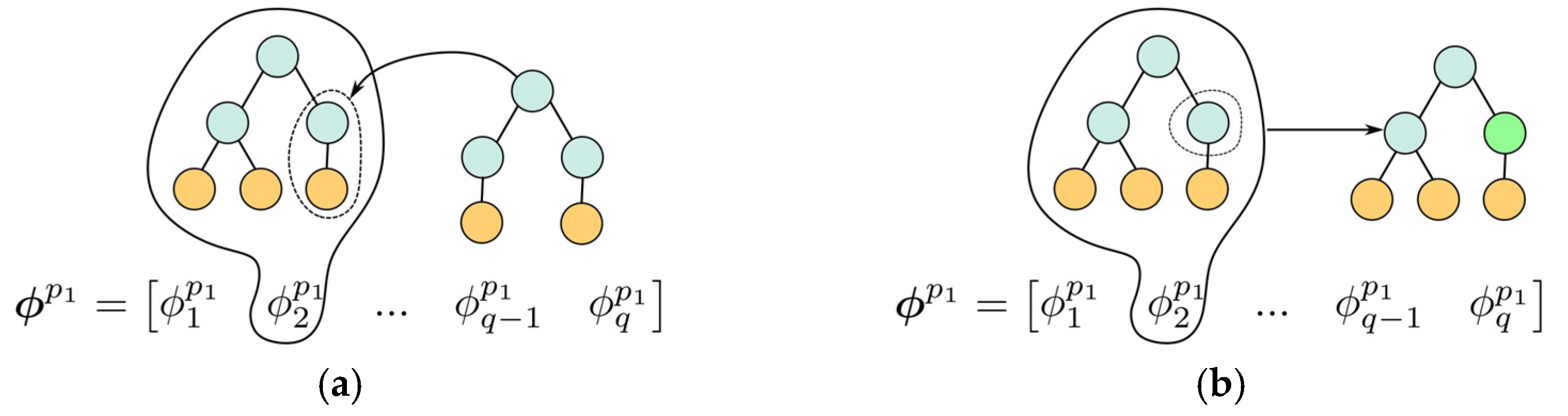The high-level crossover is a uniform crossover in which 1 to $k_{max}$ trees comprising the individual are selected with equal probability and swapped, where $k_{max}$ is a hyperparameter which limits the number of trees which can be crossed over in a single high-level crossover operation. It is important that the number of trees selected for both parents be equal, which is a difference between high-level crossover in G3P-SR and MGGP, so that the number of model terms in the individual remains constant. Figure 2 is an illustration of how the model terms are swapped during high-level crossover and the subtrees of the model terms are swapped during subtree crossover.

The mutation operator ${{\rm Y}}_M:\mathcal{I}\to \mathcal{I}$ is a stochastic unitary operator that takes the individual $p_i^j$ and perturbs it to output a new individual${\tilde{p}}_i^{j+1}$. In subtree mutation, a parent tree $p_i^j$ is selected, a nonterminal node $A\in p_i^j$ is selected, and a new tree is randomly generated with the root node of the randomly generated tree matching the nonterminal node selected from $p_i^j$. The subtree below the selected node of $p_i^j$ is deleted and replaced with the newly generated tree. In point mutation, a terminal node is selected and replaced with another terminal node while making sure that the resulting offspring is syntactically correct. Figure 3 shows an illustration of subtree and point mutation.

Since the individual in G3P-SR is composed of multiple model terms represented by trees, there is a selection process not only for the individual from the population but also a selection of the model terms that will undergo subtree crossover, subtree mutation, or point mutation. The model terms are selected from each parent with a probability that is proportional to its coefficient to bias the variation step [30]. In order to obtain the probability of selecting a model term, the coefficients are first normalized using (3) and then the probability of model term i being selected is given in (4).

$$\overline{{\theta }_i}=\frac{{\sum }_{i=1}^q\left|{\theta }_i\right|-\left|{\theta }_i\right|}{{\sum }_{i=1}^q\left|{\theta }_i\right|}$$

(3)

$$P=\frac{\exp \overline{{\theta }_i}}{{\sum }_{i=1}^q\exp {\overline{\theta }}_i}$$

(4)

2.3. Regularization

Once an individual j is generated by the evolutionary process, the semantics of the model terms are stored in a design matrix ${\varphi }_j$, and sparse regression is applied in order to select the appropriate model terms and obtain their coefficients. In this paper, the l₀-penalized linear least squares problem is used:

$$L\left(\theta \right)=f\left(\theta \right)+g\left(\theta \right)=\frac{1}{2}{‖y-\varphi \theta ‖}_2^2+\lambda {‖\theta ‖}_0$$

(5)

where the vector is $y\in R^n,$ and the design matrix is $\varphi \in R^{n\times q}$. This problem has been proven to be NP-hard [39], and approximations to (5) have been based on greedy algorithms or relaxation. One commonly applied method of relaxation is basis pursuit denoising (BPDN), which replaces the $l_0$penalty with the convex $l_1$ penalty. Other methods of solving (5) include sequential threshold least squares [40], which has been used to find sparse dynamical models from a library of candidate functions, and sparse relaxed regularized regression (SR3) [41]. The mAPG algorithm was developed in [35] to find a critical point of a function $F\left(\theta \right)=f\left(\theta \right)+g\left(\theta \right)$, where it is a proper function with Lipschitz continuous gradients, $g\left(\theta \right)$ is nonsmooth and can be either convex or nonconvex but is lower semicontinuous, and $f\left(\theta \right)+g\left(\theta \right)$ is coercive. These assumptions are satisfied in (5) and, therefore, every accumulation point obtained by Algorithm 1 is a critical point of (5). A proof that the accumulation point of Algorithm 1 is a critical point of $f\left(\theta \right)+g\left(\theta \right)$, satisfying the aforementioned assumptions, can be found in [35]. Monotone accelerated proximal gradient descent is an extension of APG developed in [42], which extends Nesterov’s accelerated gradient descent to the nonsmooth case.

Algorithm 1: mAPG

Input:    $\varphi ,y,\lambda$

Initialize:   $\rho <1, \delta ,{\mathit{z}}_1={\mathit{\theta }}_1={\mathit{\theta }}_0,{ t}_1={1, t}_0=0, k=1$

while not converged do

$k\leftarrow k+1$

$w_k={\theta }_k+\frac{t_{k-1 }}{t_k}\left(z_k-{\theta }_k\right)+\frac{t_{k-1}-1}{t_k}\left({\theta }_k-{\theta }_{k-1}\right)$

Initialize step size ${\eta }_w$ and ${\eta }_{\theta }$ using Barzilai-Borwein method

while $F\left(z_{k+1}\right)\ge F\left(w_k\right)-\delta {‖z_{k+1}-w_k‖}_2^2$ do

$z_{k+1}=\mathrm{p}\mathrm{r}\mathrm{o}{\mathrm{x}}_{{\eta }_w\lambda {‖·‖}_0}\left(w_k-{\eta }_w\nabla f\left(w_k\right)\right)$

${\eta }_w={\rho \eta }_w$

end while

while $F\left(v_{k+1}\right)\ge F\left({\theta }_k\right)-\delta {‖v_{k+1}-{\theta }_k‖}_2^2$ do

$v_{k+1}=\mathrm{p}\mathrm{r}\mathrm{o}{\mathrm{x}}_{{\eta }_{\theta }\lambda {‖·‖}_0}\left({\theta }_k-{\eta }_{\theta }\nabla f\left({\theta }_k\right)\right)$

${\eta }_{\theta }={\rho \eta }_{\theta }$

end while

$t_{k+1}=\frac{\sqrt{4t_k^2+1}+1}{2}$

${\theta }_{k+1}=\left\{\begin{array}{c}{z}_{k+1}\\ v_{k+1}\end{array}\right.\begin{array}{l}\mathrm{i}\mathrm{f} F\left(z_{k+1}\right)\le F\left(v_{k+1}\right)\\ \mathrm{o}\mathrm{t}\mathrm{h}\mathrm{e}\mathrm{r}\mathrm{w}\mathrm{i}\mathrm{s}\mathrm{e}\end{array}$

end while

Output:  $\theta$

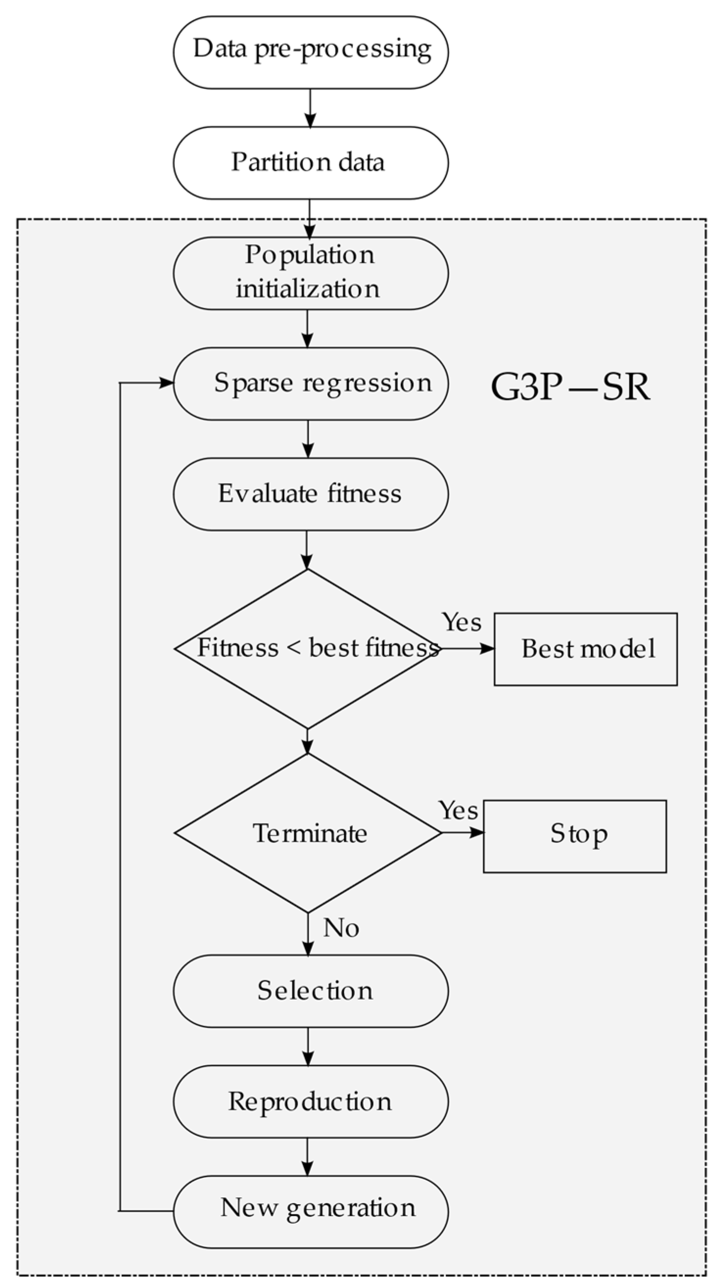
Algorithm 1 shows the implementation of mAPG. mAPG monitors the extrapolated variable w and corrects it when it has the possibility to fail while also ensuring convergence to a critical point of (5). In this work, we use a backtracking line search initialized with the Barzilai-Borwein method to find the initial step size $\eta$. The proximal operator for the $l_0$ pseudo-norm (Algorithm 1) is the hard thresholding operator (6). The flowchart of the proposed G3P-SR algorithm is shown in Figure 4.

$${\mathrm{p}\mathrm{r}\mathrm{o}\mathrm{x}}_{\gamma {‖·‖}_0}v=\left\{\begin{array}{c}\begin{array}{cc}0& \left|v\right|\le \sqrt{2\gamma }\end{array}\\ \begin{array}{cc}\upsilon & \left|v\right|>\sqrt{2\gamma }\end{array}\end{array}\right.$$

(6)

2.4. NARX-NN and TSF-ARX Models

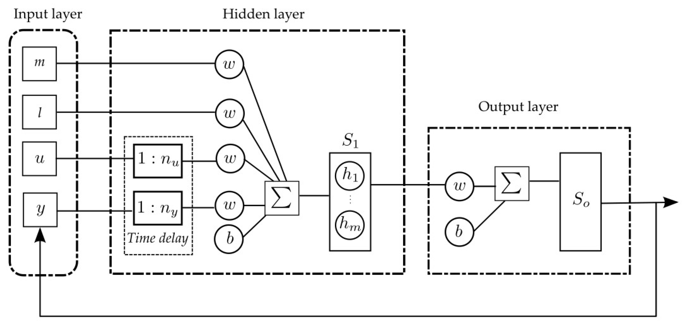
A nonlinear autoregressive neural network with exogenous inputs (NARX-NN) and Takagi-Sugeno fuzzy (TSF-ARX) models has been chosen in this study for a comparative analysis. The NARX-NN is a recurrent dynamic network with output feedback. The architecture of the NARX-NN model of the crane dynamic used for the comparative analysis is shown in Figure 5, where l and m are, respectively, the rope length and the mass of the payload transported by a crane, which indicate the current operating point of a crane system, while u and y are the input signal and the model response, respectively. The time-delayed normalized inputs and outputs are fed into the hidden layer, where a linear combination of inputs passes through an activation function. Throughout this work, the activation function has been chosen as the tangent-sigmoid function, while the output function is linear. The weights w and biases b have been optimized using the Levenberg–Marquardt algorithm. The optimization process is halted if the maximum number of epochs exceeds 1000, the gradient is less than 10⁻⁷, or the MSE on the validation data set increases six times consecutively.

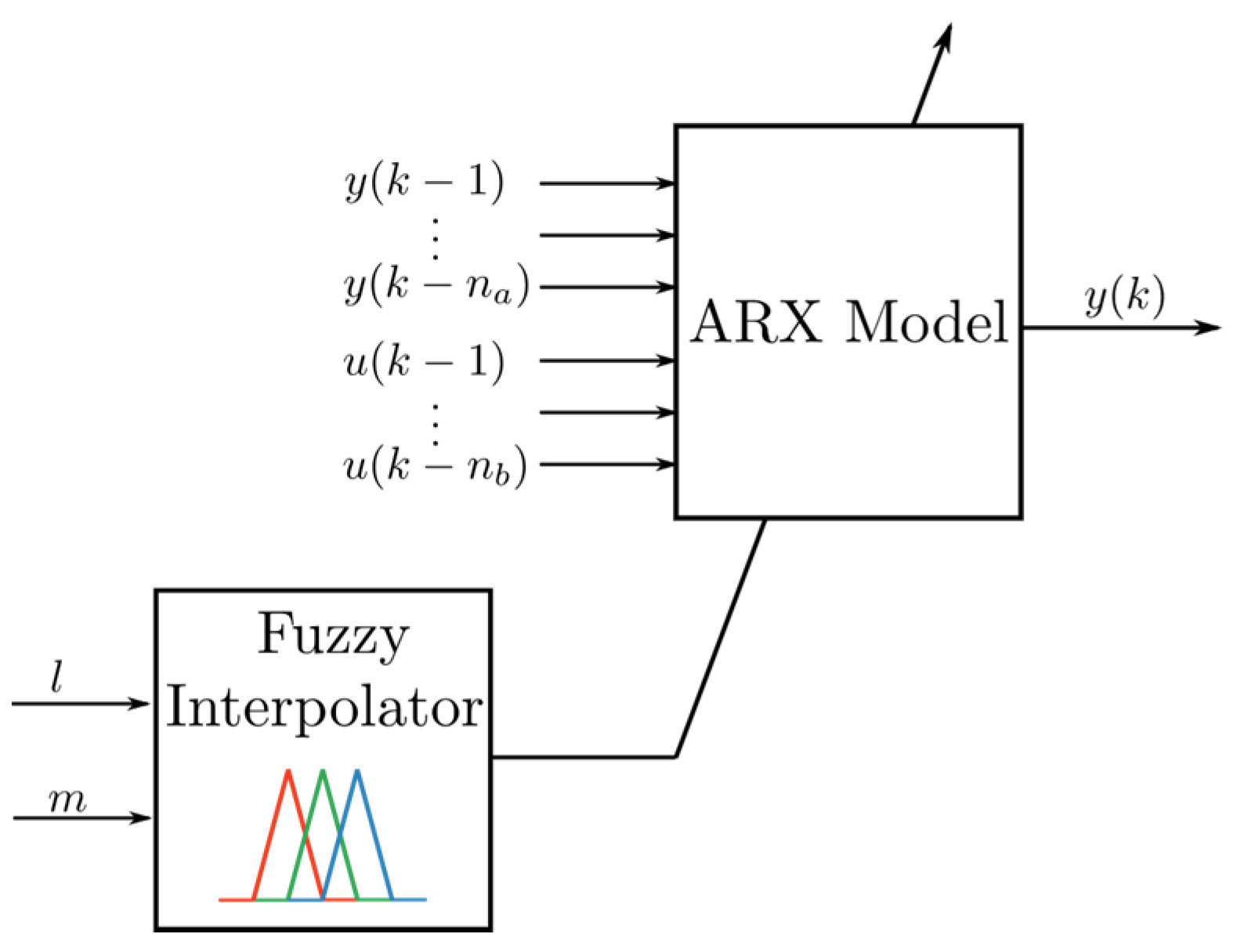
Linear models offer several advantages such as ease of implementation in addition to increased interpretability but lack the flexibility required to model complex systems. One method to overcome this has been to use local linear methods by partitioning the input space into several operating points in which the system can be represented by a parameter varying (LPV) linear model. An LPV-ARX system is described by

$$y_k+\sum _{i=1}^{n_a}{a}_i\left(l,m\right)y_{k-i}=\sum _{j=0}^{n_b}{b}_i\left(l,m\right)u_{k-j}+e_k$$

(7)

where the coefficients of the ARX model are dependent on the scheduling variables, rope length l, and mass of a payload m, which indicate the current operating point of a crane system. The parameters of the ARX model for a given operating point are found using the least squares method, and a Takagi-Sugeno fuzzy system is applied to interpolate between the locally linear models. Figure 6 shows a description of the TSF-ARX model used for our comparative analysis.

3. Experiment and Results

The data used in the identification procedure were obtained from experiments carried out on a laboratory double-girder crane mechanism. The mechanism was driven by two AC gear motors with a gear ratio of 15.5, operating at 1400 rpm and with an output power of 0.18 kW. The AC motors were supplied by two LG iC5 0.4 kW frequency inverters, controlled by a Mitsubishi FX2N series Programmable Logic Controller (PLC). The crane mechanism was equipped with the incremental encoders installed on the wheels to measure the position x relative to the crane bridge, under the trolley connected to a pair of fork arms within which the hoisting cable passed through to measure the sway angle α of the cable-suspended payload and on the drum of the lifting mechanism to measure the rope length l. The incremental encoders had a resolution of 400 pulses per rotation (ppr), 2000 ppr, and 100 ppr to measure the position x, sway, angle α, and rope length l, respectively. The data from the sensors were sampled at 10 Hz using a PC with 16 GB RAM and Quad Core 4 GHz Intel Core i7-6700K CPU running Windows 10 and Matlab R2020. The PLC was used during the experiments to transfer and convert the control and measurement signals exchanged between the PC with IO card and a plant. The control analog voltage signal u within the range ±10 V was sent from the PC with IO card to the PLC, which transmitted this signal to the frequency inverters converting it to the voltage signal 0–10 V and binary signals corresponding to a frequency change within the range 0–50 Hz and the direction of motor rotation, respectively. Figure 7 shows a view of the laboratory overhead crane and the data acquisition equipment used in the identification experiments.

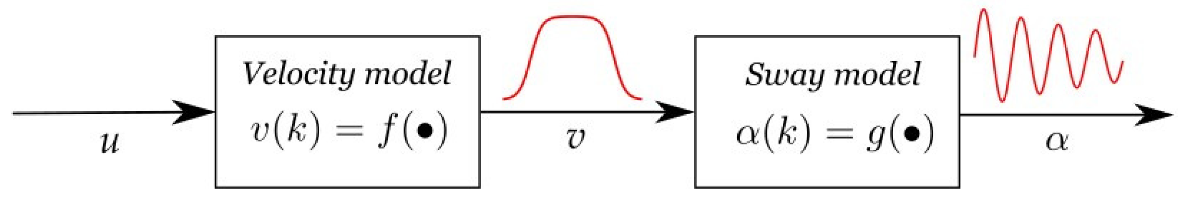
The overhead crane dynamics were assumed to be composed of two submodels, comprising the actuated and underactuated parts of the crane system, connected in series as shown in Figure 8. The first model, denoted as the velocity model, presented the relation between control signal u and crane velocity v, while the second model, denoted as the sway model, presented the relation between crane velocity v and payload sway α. This assumption was implemented in the identification experiments to derive the G3P-SR models, as well as the NARX-NN and TSF-ARX velocity and sway models used for our comparative analysis. The laboratory overhead crane was not equipped with a sensor to measure the velocity, and, therefore, a constant-velocity Kalman filter was used to estimate the velocity of the trolley. The process noise and measurement noise followed Gaussian distributions $N\left(0,{\sigma }_p^2\right)$ and $N\left(0,{\sigma }_m^2\right)$, where ${\sigma }_p=8$ and ${\sigma }_m=0.2$. Ten experiments were carried out with a varying payload mass m and rope length l. The experimental data were partitioned into three sets: the training set, which was used to minimize (5), and the MSE on the training set was used as the fitness function in G3P-SR and, therefore, drove the evolutionary process; the validation set, which was used only for model selection, i.e., the model with the lowest MSE on the validation set was stored as the best model; and the testing set, which was used to evaluate the performance of the obtained model. The training and validation sets comprised experiments 1–8, and the data were combined and split randomly with a 70:30 ratio into the training and validation sets, respectively, while experiments 9–10 were used as the testing sets. The operating points of experiments 1–8 were selected to fill the design space by maximizing the minimum distance [43] between the operating points, i.e., ${d^{*}=\underset{D}{\max }\underset{i,j}{\min }‖p_i-p_j‖}_2$, where $p_i\in [0, 1]\times \left\{\mathrm{0,0.5,1}\right\}$ was the scaled design space, as the payload mass could only take on the discrete values of $\left\{\mathrm{10,30,50}\right\}$ kg while the rope length could vary continuously in the interval $[0.8,2.0]$ m. The operating point for each experiment is given in

Table 1. Operating points of experimental data used in identification.

Operating Point	Exp 1	Exp 2	Exp 3	Exp 4	Exp 5	Exp 6	Exp 7	Exp 8	Exp 9	Exp 10
l [m]	0.8	1.4	2.0	2.0	1.7	1.4	0.8	1.1	1.7	1.1
m [kg]	10	10	50	10	30	50	50	30	10	50

. The input signal u was a sequence of step functions with varying amplitudes in order to excite the underactuated part of the overhead crane, as shown in Figure 9. The data used for identification were normalized by dividing the input sequence by 10 and the overhead crane velocity by 30.

The grammar used for representing individuals consisted of a terminal set, which included lagged input and output variables, the mass of the payload m, the rope length l, and several integers, while rational and irrational constants could be obtained by the division and square root operator, respectively. The mass of the payload m and the rope length l were assumed as the measurable parameters. The grammar constructed to derive the velocity and sway model is presented in

Table 2. Grammar used to obtain the crane velocity model.

⟨S⟩	::=	⟨expb1⟩|⟨T⟩
⟨expb1⟩	::=	×⟨expb1⟩⟨expb1⟩|×⟨expp⟩⟨expb1⟩|⟨expu⟩|⟨T⟩
⟨expu⟩	::=	tanh⟨expb2⟩|abs⟨expb2⟩
⟨expb2⟩	::=	+⟨expb2⟩⟨expb2⟩|−⟨expb2⟩⟨expb2⟩|×⟨expb2⟩⟨expb2⟩|×⟨int⟩⟨expb2⟩|⟨T⟩
⟨expp⟩	::=	×⟨expp⟩⟨expp⟩|inv⟨expp⟩|⟨Tp⟩
⟨int⟩	::=	×⟨int⟩⟨int⟩|+⟨int⟩⟨int⟩|÷⟨int⟩⟨int⟩|√⟨int⟩|⟨TI⟩
⟨T⟩	::=	vk−1|vk−2|…|vk−4|uk−1|uk−2|…|uk−9
⟨TI⟩	::=	1|2|3|5|10
⟨Tp⟩	::=	m|l

and

Table 3. Grammar used to obtain the sway model.

⟨S⟩	::=	⟨expb1⟩|⟨T⟩
⟨expb1⟩	::=	×⟨expb1⟩⟨expb1⟩|×⟨expp⟩⟨expb1⟩|⟨expu⟩|⟨T⟩
⟨expu⟩	::=	tanh⟨expb2⟩|sin⟨expb2⟩|cos⟨expb2⟩|tan⟨expb2⟩
⟨expb2⟩	::=	+⟨expb2⟩⟨expb2⟩|−⟨expb2⟩⟨expb2⟩|×⟨expb2⟩⟨expb2⟩|×⟨int⟩⟨expb2⟩|⟨T⟩
⟨expp⟩	::=	×⟨expp⟩⟨expp⟩|inv ⟨expp⟩|⟨Tp⟩
⟨int⟩	::=	×⟨int⟩⟨int⟩|+⟨int⟩⟨int⟩|÷⟨int⟩⟨int⟩|√⟨int⟩|⟨TI⟩
⟨T⟩	::=	αk−1|αk−2|…|αk−4|vk−1| vk−2|…|vk−8
⟨TI⟩	::=	1|2|3|5|10
⟨Tp⟩	::=	m|l

, respectively, using the Backus–Naur form (BNF) [33], while the G3P-SR hyperparameters used to obtain both models are given in

Table 4. G3P-SR hyperparameters.

Parameters	Values
Population size	100
Number of generations	500
Initialization method	PTC2
Max tree depth during initialization	6
Max number of candidate model terms	50
Tournament size	2
Subtree crossover probability	0.75
High-level crossover probability	0.15
Mutation probability	0.1
Max number of prox. evaluations iterations	5000

.

The comparative study was divided into two parts. In the first part, we discussed the choice of the $\lambda$ hyperparameter value and compared the performance of the proposed approach with MGGP. The second part provided a comparison of the G3P-SR method with the crane dynamic models developed using the most commonly used approaches in the crane identification literature—ANN and TSF.

3.1. λ Hyperparameter Selection

In (5), hyperparameter $\lambda$ determines the level of sparsity of the coefficient vector $\theta$ and, therefore, needs to be selected appropriately. In this section, we compare optimizing hyperparameter $\lambda$ based on grid search 3-fold cross-validation and setting a constant $\lambda$, which was selected empirically, throughout the G3P-SR run. In the case of the grid search, it was important to determine the value of $\lambda$ for which the zero vector would be a critical point of (5). Since the model terms’ initial values were set to zero, we obtained

$$\eta {\varphi }^{T}y\le \sqrt{2\lambda \eta }$$

(8)

The step size $\eta$ was not constant in Algorithm 1, but, since the initial value was chosen to be $\eta =1/L$, where $L$ was the Lipschitz constant which, for (5), was given by $L={\sigma }_{max}{\left(\varphi \right)}^2$,where ${\sigma }_{max}\left(·\right)$ was the largest singular value, we could obtain

$$\lambda \ge \frac{\eta \max {\left({\varphi }^{T}y\right)}^2}{2}$$

(9)

Therefore, in the interval $0\le \lambda <\frac{\eta \max {\left({\varphi }^{T}y\right)}^2}{2}$, we had a non-zero vector of model term coefficients. For the 3-fold cross validation, four values of $\lambda$ were chosen, logarithmically spaced, from the interval $\frac{\eta \min {\left({\varphi }^{T}y\right)}^2}{2}\le \lambda \le 0.65\frac{\eta \max {\left({\varphi }^{T}y\right)}^2}{2}$. The coefficient 0.65 was chosen, as values closer to the limit $\frac{\eta \max {\left({\varphi }^{T}y\right)}^2}{2}$ tend to have very few model terms included. In order to promote sparsity, the value of $\lambda$ chosen from the 3-fold CV was the value within one standard deviation from $\lambda$ that resulted in the minimum MSE.

To determine if the 3-fold CV resulted in better models for describing crane dynamics as opposed to a constant $\lambda$, a total of 10 runs were carried out for the identification of the crane velocity submodel, with the constant $\lambda =0.001$. The Wilcoxon rank sum test was performed to determine if the medians of the RMSE obtained with a constant $\lambda$ or $\lambda$ obtained via cross-validation were equal under the null hypothesis. The p-values are summarized in

Table 5. p-values given by the Wilcoxon rank sum test.

	l = 1.7 [m], m = 10 [kg]	l = 1.1 [m], m = 50 [kg]
1-step ahead	1.000	0.9097
10-step ahead	0.6776	0.2730
20-step ahead	0.4274	0.3075

for 1-step ahead, 10-step ahead, and 20-step ahead for test sets with operating points $l=1.7 \mathrm{m}$ and $m=10$ kg and $l=1.1$ m and $m=50$ kg, respectively.

Since the null hypothesis could not be rejected, and the mean runtime was 11.35 min and 99.6 min for the constant hyperparameter $\lambda$ and the hyperparameter $\lambda$ obtained by the 3-fold CV, respectively, a constant value of the hyperparameter $\lambda$ was used for all future runs with $\lambda =0.001$ and $\lambda =0.0005$ for the velocity and sway submodels, respectively.

3.2. Comparison with MGGP

To show the efficacy of G3P-SR, a comparison between G3P-SR and MGGP was performed with the MGGP hyperparameters given in

Table 6. MGGP hyperparameters.

Parameters	Velocity Model	Sway Model
Function set	$\times ,+,-,÷,\mathrm{t}\mathrm{a}\mathrm{n}\mathrm{h},\sqrt{ }, \left| \right|$	$\times ,+,-,÷,\mathrm{t}\mathrm{a}\mathrm{n}\mathrm{h},$ $\sqrt{ },\mathrm{s}\mathrm{i}\mathrm{n},\mathrm{c}\mathrm{o}\mathrm{s},\tan$
Terminal set	$u_{k-1},\dots ,u_{k-9},$ $v_{k-1},\dots , v_{k-4},$  $m, l$	$v_{k-1},\dots ,v_{k-8},$ ${\alpha }_{k-1},\dots , {\alpha }_{k-4},$ $m, l$
Population size	100
Number of generations	500
Initialization	Ramped Half-and-Half
Maximum number of genes	50
Maximum tree depth	5
Tournament size	5
Elitism	0.01
Crossover probability	0.84
Mutation probability	0.14
Direct reproduction	0.02
Ephemeral random constant	[−10, 10]

. The G3P-SR algorithm was implemented in Matlab 2021a, and the GPTIPS 2.0 toolbox for Matlab was used to obtain the MGGP model. The models were evaluated for the 1-step ahead, 10-step ahead, 20-step ahead predictors and a simulation run. The model obtained was trained in a series-parallel configuration and, therefore, minimized the 1-step-ahead prediction; while this resulted only in an approximation of k-step-ahead predictions and simulations, it was faster than training the model in a series configuration, i.e., performing simulation error minimization. A total of 15 runs were performed for the velocity and sway submodels with G3P-SR and MGGP, and the Wilcoxon rank sum test was used to determine if the medians of the RMSE between the G3P-SR and MGGP models were different under the alternative hypothesis. The p-values for the velocity and sway submodels are given in

Table 7. p-values for comparison of the RMSE of G3P-SR and MGGP.

	Velocity Submodel		Sway Submodel
	l = 1.7 [m] m = 10 [kg]	l = 1.1 [m] m = 50 [kg]	l = 1.7 [m] m = 10 [kg]	l = 1.1 [m] m = 50 [kg]
1-step ahead	9.0465 × 10−4	0.0512	7.7915 × 10−4	0.0014
10-step ahead	0.0279	0.0025	0.4067	0.0225
20-step ahead	0.0251	0.0054	0.5614	0.0042

Remark: Bold denotes statistically significant values.

, and the boxplots of the RMSE for the 1-step-, 10-step-, and 20-step-ahead predictors on test with operating points $l=1.7 \mathrm{m}$ and $m=10$ kg and $l=1.1$ m and $m=50$ kg, denoted as T₁ and T₂, respectively, for the velocity and sway submodels are given in Figure 10 and Figure 11, respectively, while the boxplot for the number of model terms included in the models is given in Figure 12.

For the velocity submodel, at operating point l = 1.7 m and m = 10 kg, the MGGP median RMSE for the 1-step, 10-step, and 20-step predictors was 3.77%, 4.96%, and 10.40% higher than the G3P-SR median RMSE, respectively. At operating point l = 1.1 m and m = 50 kg, the MGGP median RMSE was 1.45%, 6.94%, and 4.00% higher than the G3P-SR median RMSE, respectively. The Wilcoxon rank sum test showed that the difference between the MGGP and G3P-SR 1-step-ahead median RMSE for operating point l = 1.1 m and m = 50 kg was not statistically significant, with a p-value of 0.0512. For the sway submodel, at operating point l = 1.7 m and m = 10 kg, the MGGP median RMSE for the 1-step, 10-step, and 20-step predictors was 4.00%, 6.41%, and 10.00% higher than the G3P-SR median RMSE, respectively. At operating point l = 1.1 m and m = 50 kg, the MGGP median RMSE was 9.09%, 14.61%, and 12.40% higher than the G3P-SR median RMSE, respectively. However, the Wilcoxon rank sum test showed that the difference between the MGGP and G3P-SR 10-step and 20-step ahead for operating points l = 1.7 m and m = 10 kg were not statistically significant, with p-values of 0.4067 and 0.5615, respectively. The median number of velocity model terms in the G3P-SR and MGGP models was 25 and 47, respectively, while the median number of sway model terms in the G3P-SR and MGGP models was 27 and 49, respectively. The mean run times of the velocity submodel were 11.2 min and 7.5 min for the G3P-SR and MGGP algorithms, respectively. The mean run times of the sway submodel were 10.7 min and 9.2 min for the G3P-SR and MGGP algorithms, respectively. Additionally, the obtained models were simulated, and all G3P-SR models were finite, while the MGGP algorithm produced 3 unstable sway models and 10 unstable velocity models. The G3P-SR algorithm produced models that had a better or similar accuracy, were more parsimonious, and were stable during simulation compared to the MGGP models but at the cost of increased computational times. For these reasons, only the G3P-SR model was used in the comparative analysis described in the next section.

3.3. Comparison with NARX-NN and TSF-ARX Models

The G3P-SR algorithm was compared with the NARX-NN and TSF-ARX models. The number of input delays for both submodels, as well as the number of output delays for the velocity submodel of the NARX-NN (Figure 5), was chosen to be of the same order as that for the G3P-SR. The NARX-NN sway submodel required an additional delay $\alpha \left(k-5\right)$, as the results with only four output delays were unsatisfactory. The structures of NARX-NN with three, four, and five hidden neurons were tested for the velocity model, while, for the sway model, the number of hidden nodes was chosen to be three, five, and six.

The appropriate number of input and output delays for the local linear models (7) of the TSF-ARX system (Figure 6) was found using the minimum description length (MDL) criterion implemented in MATLAB’s system identification toolbox, which resulted in the velocity and sway models given in (10) and (11), respectively. The coefficients were computed using the linear least squares method at the operating points, and a linear membership function was used to interpolate between the linear models.

$$v_k+a_1^1\left(l,m\right)v_{k-1}+\cdots +a_4^1\left(l,m\right)v_{k-4}=b_1^1{u}_{k-4}$$

(10)

$${\alpha }_k+a_1^2\left(l,m\right){\alpha }_{k-1}+\cdots +a_6^2\left(l,m\right){\alpha }_{k-6}=b_1^2{v}_{k-1}+b_2^2{v}_{k-2}$$

(11)

The model terms and their corresponding coefficients for the sway and velocity model obtained in identification experiments using the G3PSR are given in

Table 8. Sway model terms and coefficients.

Velocity Submodel		Sway Submodel
Coefficients	Model Terms	Coefficients	Model Terms
0.0336	$\tanh \left(6\left(u_{k-2}+u_{k-3}\right)\right)$	0.4363	${\alpha }_{k-2}$
0.0220	$\tanh \left(v_{k-2}+10v_{k-7}\right)$	4.7829 × 10−4	$l^2{v}_{k-5}$
−0.0362	$\tanh \left(u_{k-1}+13\left(v_{k-2}-u_{k-5}\right)\right)$	−6.8103 × 10−4	$l^2\cos \left({\alpha }_{k-1}\right)$
0.2790	$\tanh \left(v_{k-1}+u_{k-8}\right)$	−1.4753	$\tanh \left(\frac{\sqrt{2}{\alpha }_{k-2}}{9}\right)$
0.1168	$v_{k-2}$	0.0992	$m{\alpha }_{k-1}{\alpha }_{k-3}\sin \left({\alpha }_{k-1}\right)$
0.0037	$u_{k-4}{u}_{k-6}$	−0.0023	$\tanh \left(10\left(v_{k-1}-v_{k-2}\right)\right)$
−0.0106	$\left|u_{k-6}-u_{k-9}\right|$	−0.0510	$l^{-1}\cos \left({\alpha }_{k-1}\right)\tanh \left(v_{k-1}-v_{k-2}\right)$
−0.0255	$\tanh \left(5v_{k-3}\right)$	−0.0056	$\tanh \left(2{\alpha }_{k-4}-v_{k-2}+2v_{k-4}\right)$
−0.0863	$\tanh \left(6\left(u_{k-2}+v_{k-1}\right)\right)$	1.0111	$\tan \left({\alpha }_{k-1}\right)$
0.6076	$v_{k-1}$	0.0034	$l^{-1}{v}_{k-1}$
−0.1075	$u_{k-1}\tanh \left(u_{k-3}\right)\tanh \left(u_{k-6}\right)$	−0.1581	$l^{-1}{\alpha }_{k-2}$
0.0248	$\tanh \left({u_{k-1}u}_{k-3}{u}_{k-9}-\frac{8}{3}{u}_{k-8}\right)$	−0.0015	$l^{-2}\cos \left({\alpha }_{k-1}\right)$
0.0045	$\tanh \left(4u_{k-2}\right)$	−0.2316	${\alpha }_{k-4}$
0.0313	$u_{k-9}$	−0.0941	$m{\alpha }_{k-1}\sin \left({\alpha }_{k-1}\right)\tanh \left({\alpha }_{k-2}\right)$
−0.1743	$u_{k-8}$	−0.0011	$l^{-1}\cos \left({\alpha }_{k-1}\right)$
0.0067	$\mathrm{t}\mathrm{a}\mathrm{n}\mathrm{h}\left(u_{k-1}{v}_{k-2}\right(100v_{k-2}+u_{k-9}\left)\right)$	−0.0123	$m\sin \left({\alpha }_{k-1}\right)\tanh \left(10v_{k-1}{\alpha }_{k-1}\right)\tanh \left(\frac{\sqrt{2}{\alpha }_{k-4}}{9}\right)$
0.0582	$u_{k-6}$	8.4577 × 10−4	$\tanh \left(3v_{k-1}{\alpha }_{k-1}\right)$
−2.2057 × 10−5	$m{l}^2{v}_{k-1}{v}_{k-2}{u}_{k-1}{u}_{k-4}{u}_{k-5}$	0.4044	$\sin \left({\alpha }_{k-1}\right)\tanh \left(\frac{\sqrt{2}{\alpha }_{k-4}}{9}\right)\tanh \left(4v_{k-5}\right)$
0.1596	$v_{k-1}{u}_{k-8}{u}_{k-9}$	0.0013	$\tanh \left(10v_{k-1}{v}_{k-2}{v}_{k-4}\right)$
−0.0210	$\tanh \left(\frac{9}{2}\sqrt{3}{u}_{k-5}\right)$	4.6043 × 10−7	$m^2\cos \left({\alpha }_{k-1}\right)$
−0.0176	$\tanh \left(5u_{k-5}-100u_{k-9}+u_{k-2}\right)$	0.0043	${\left(\sqrt{\frac{l}{m}}\cos \left({\alpha }_{k-1}\right)\right)}^{-1/2}$
0.0237	$\tanh \left(13\left(v_{k-2}-20u_{k-9}\right)+u_{k-1}\right)$	0.0023	$\frac{1}{\sqrt{m}}\cos \left({\alpha }_{k-1}\right)$
0.0455	$\tanh \left(6u_{k-2}{u}_{k-4}\right)$	−0.0047	$m{\alpha }_{k-1}\sin \left({\alpha }_{k-1}\right)\tanh \left(v_{k-6}\right)$
0.0828	$\tanh \left(v_{k-2}{u}_{k-1}\left(u_{k-7}+u_{k-9}\right)\right)$

. We notice that the mass of the payload m and rope length l appear in only one model term for the velocity as opposed to fourteen model terms for the sway; this is due to the high mechanical impedance of the crane mechanism leading to the payload having a miniscule impact on the velocity of the trolley.

All the identification methods presented in this work were trained in a series-parallel configuration, resulting in a 1-step-ahead predictor. The k-step-ahead predictor was obtained by placing k number of 1-step-ahead predictors in a series, in which the predicted output $\widehat{y}\left(k-i-1\right)$ of the ith predictor was the input into the (i + 1)th predictor, where $1\le i<k$. The simulation was obtained by closing the loop and using the measured outputs only as the initial states. The models’ performances for the 1-step-, 10-step-, 20-step-ahead predictions and for the simulations evaluated on the testing data using the MSE, as well as the complexity of the models (the number of parameters to be estimated P), are presented in

Table 9. Models’ performances for crane velocity and payload sway prediction.

		Crane Velocity Prediction			Payload Sway Prediction
		l = 1.7 [m] m = 10 [kg]	l = 1.1 [m] m = 50 [kg]			l = 1.7 [m] m = 10 [kg]	l = 1.1 [m] m = 50 [kg]
		MSE		P		MSE		P
1-step-ahead	G3P-SR	3.0291 × 10−5	5.2661 × 10−5	24	G3P-SR	6.4286 × 10−6	4.9985 × 10−6	23
10-step-ahead		1.3830 × 10−4	2.7134 × 10−4			6.4842 × 10−5	5.3106 × 10−5
20-step-ahead		1.4942 × 10−4	2.7561 × 10−4			6.0479 × 10−5	1.2444 × 10−4
simulation		1.0225 × 10−4	1.1860 × 10−4			4.8531 × 10−4	3.0533 × 10−4
1-step-ahead	NARX-NN3	7.8298 × 10−5	9.8596 × 10−5	52	NARX-NN3	9.3471 × 10−6	1.0445 × 10−5	52
10-step-ahead		2.9076 × 10−4	4.1626 × 10−4			5.6156 × 10−5	8.2768 × 10−5
20-step-ahead		3.0742 × 10−4	4.3185 × 10−4			7.5216 × 10−5	2.6174 × 10−4
simulation		2.9124 × 10−4	4.0581 × 10−4			0.0019	0.0038
1-step-ahead	NARX-NN4	4.3865 × 10−5	7.0114 × 10−5	69	NARX-NN5	9.3449 × 10−6	7.3236 × 10−6	86
10-step-ahead		1.7400 × 10−4	2.1771 × 10−4			5.3269 × 10−5	2.4832 × 10−5
20-step-ahead		1.9878 × 10−4	2.1986 × 10−4			5.8469 × 10−5	5.2031 × 10−5
simulation		1.8707 × 10−4	2.0629 × 10−4			0.0018	8.8766 × 10−4
1-step-ahead	NARX-NN5	4.3021 × 10−5	6.6277 × 10−5	86	NARX-NN6	1.1624 × 10−5	1.2822 × 10−5	103
10-step-ahead		1.4043 × 10−4	1.5458 × 10−4			1.4221 × 10−4	1.4785 × 10−4
20-step-ahead		1.4161 × 10−4	1.5593 × 10−4			4.5941 × 10−5	4.3153 × 10−5
simulation		1.3297 × 10−4	1.4595 × 10−4			4.8571 × 10−4	1.1371 × 10−4
1-step-ahead	TSF-ARX	4.4354 × 10−5	4.7230 × 10−5	30	TSF-ARX	5.7590 × 10−6	5.3920 × 10−6	48
10-step-ahead		6.3366 × 10−4	6.8210 × 10−4			5.9411 × 10−5	1.3500 × 10−4
20-step-ahead		6.3176 × 10−4	6.5438 × 10−4			1.2428 × 10−4	4.0738 × 10−4
simulation		6.4512 × 10−4	6.5970 × 10−4			8.2410 × 10−4	0.0025

.

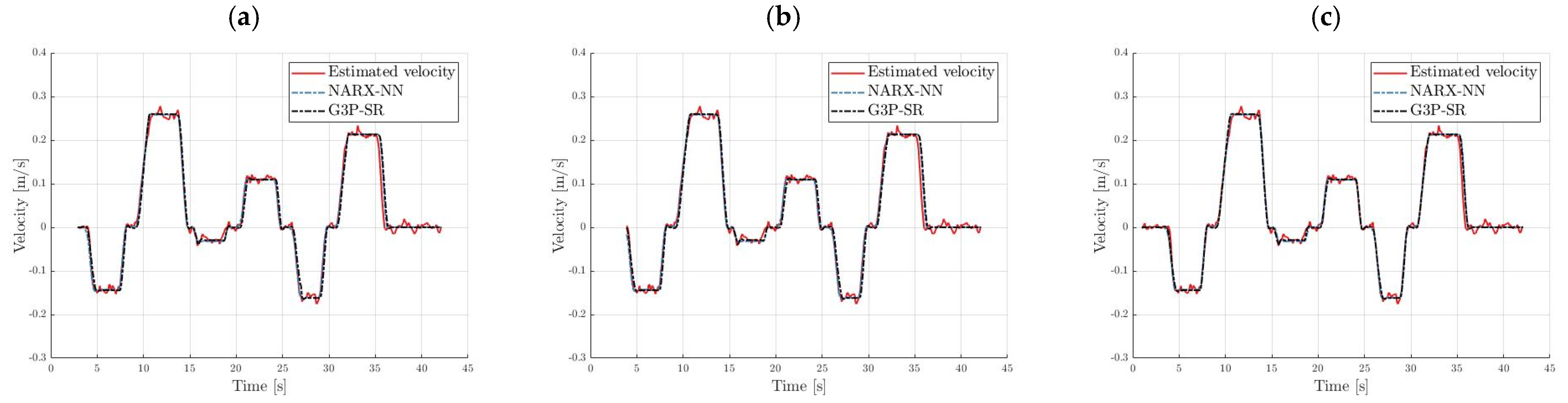
The crane velocity model obtained from the G3P-SR algorithm had the lowest complexity, with a total of 24 estimated non-zero parameters, as opposed to the 52, 69, and 86 for the NARX-NN with three, four, and five neurons in the hidden layer, respectively, and 30 for the TSF-ARX. The NARX-NN with five hidden neurons had the best 20-step-ahead prediction accuracy on both test sets at the expense of having 86 parameters in the model, while the G3P-SR algorithm produced the velocity model with the best simulation accuracy on both test sets while also having the least number of parameters in the model. 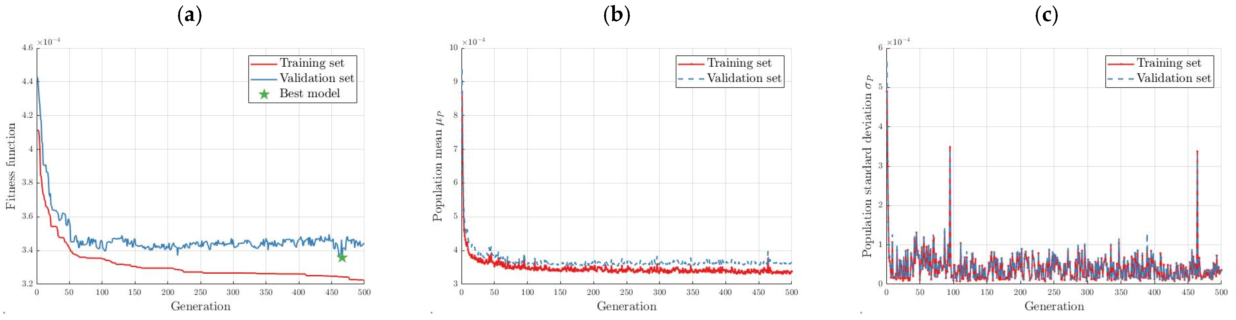The NARX-NN with five hidden neurons outperformed the TSF-ARX and the remaining NARX-NN models; therefore, it was the only model compared with the G3P-SR model output on the data from experiment 9 in Figure 13 and the data from experiment 10 in Figure 14. The fitness function for the training and validation data for the G3P-SR crane velocity model is shown in Figure 15a. The algorithm seemed to have plateaued at around 100 generations, but the best model was found in the 466th generation. The semantic diversity computed as the standard deviation of the population at a given generation is shown in Figure 15c.

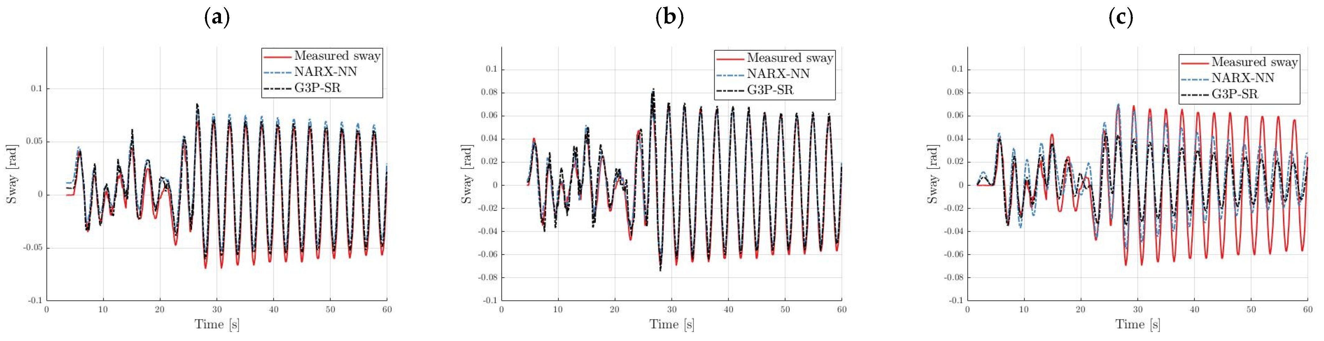
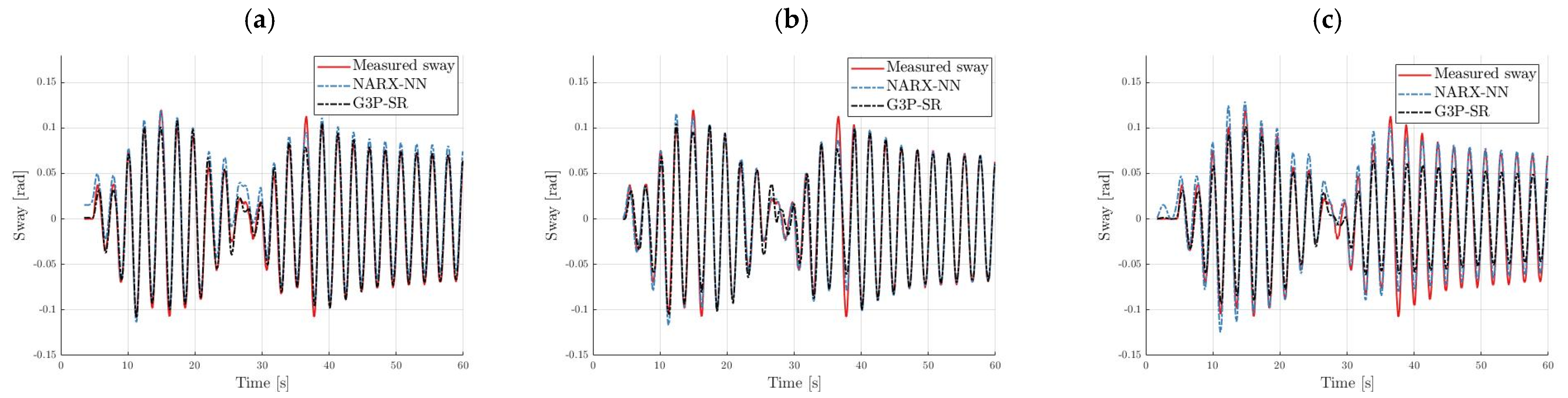
The G3P-SR and TSF-ARX sway models had 23 and 48 parameters, respectively, while the complexity of the NARX-NN model increased from 52 to 103 parameters with the increase in the number of hidden neurons from three to six. The TSF-ARX model performed poorly on the 20-step predictions and simulations on both testing sets but provided a comparable 1-step-ahead prediction accuracy to the G3P-SR model. The G3P-SR had a similar 20-step prediction accuracy to the neural network model with five hidden neurons but was more accurate during the simulations. The neural network model with six hidden neurons had the best 20-step-ahead prediction accuracy but had the highest complexity in terms of the number of parameters to be estimated; therefore, the slightly worse results of the G3P-SR model were compensated by the significant reduction in complexity, which made the model more feasible, e.g., for model-predictive control applications. 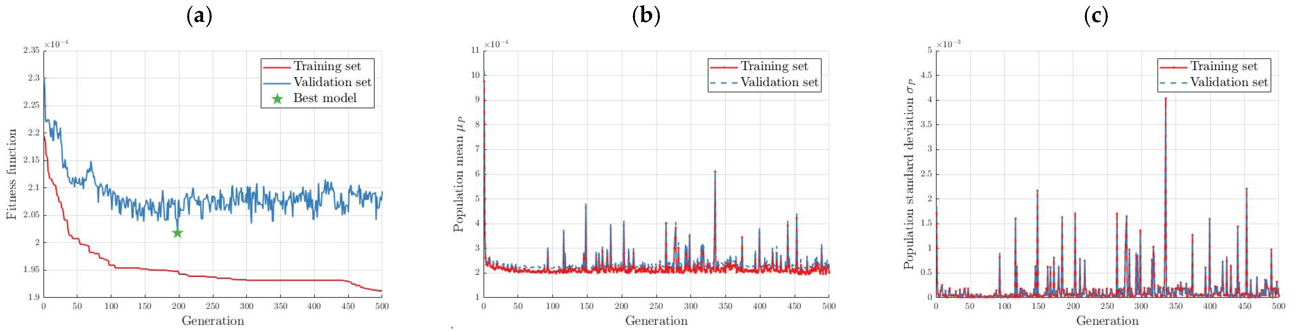Figure 16 and Figure 17 show the 10-step, 20-step, and simulation run for the NARX-NN with six hidden neurons and the G3P-SR models for the testing data. The values of the fitness function for both the normalized training and validation data sets are shown in Figure 18a. The best model was found in the 198th generation. The population mean and standard deviations are shown in Figure 18b and Figure 18c, respectively. The population experienced more semantic diversity than in the run with the velocity model, with the standard deviation being greater by about a factor of 10.

3.4. Sensitivity Analysis

A sensitivity analysis was used to determine the effect of the rope length and payload mass on the sway model output on for both the NARX-NN with six hidden neurons and the G3P-SR models. The elementary effect (EE) method was applied to perform a global sensitivity analysis. The EE method consists of generating a series of R trajectories, where each trajectory is composed of $k+1$ points, where k is the number of input variables to be varied. The inputs are then perturbed one factor at a time (OAT) by a step $\mathsf{\Delta }$, as shown in (12), and require a total of $R\left(k+1\right)$ model evaluations.

$$E{E}_i\left(x\right)=\frac{f\left(x_1^j,\dots ,x_{i-1}^j,x_i^j+\mathsf{\Delta },x_{i+1}^j,\dots ,x_k^j\right)-f\left(x_1^j,\dots ,x_{i-1}^j,x_i^j,x_{i+1}^j,\dots ,x_k^j\right)}{\mathsf{\Delta }}$$

(12)

The sample mean ${\mu }_i^{*}$ of the absolute value of the elementary effects as well as the standard deviation ${\sigma }_i$ are computed using (13) and (14), respectively, which gives us a measure of the contribution of each parameter and an estimate of the nonlinear effects of the parameter.

$${\mu }_i^{\mathrm{*}}=\frac{1}{R}{\sum }_{j=1}^R\left|E{E}_i\left(x^j\right)\right|$$

(13)

$${\sigma }_i=\sqrt{{\sum }_{j=1}^R\frac{{\left(E{E}_i\left(x^j\right)-{\mu }_i\right)}^2}{R}}$$

(14)

The mean and standard deviation of the elementary effects of the rope length and mass are displayed in Figure 19 and Figure 20, respectively. The mean of the elementary effect of the payload mass was greater in the NARX-NN model compared to the G3P-SR model, indicating that the G3P-SR model was more robust to changes in the payload mass. The mean of the elementary effect of the rope length was slightly larger in the G3P-SR model. In both cases, it was noticeable that the model was less sensitive during the transient state when the trolley was in motion and the residual oscillations were more sensitive to parameter changes. The mean of the elementary effect of both models was greater by about two orders of magnitude than that of the mean elementary effect of the payload mass; thus, we can conclude that both models are robust to changes in the payload mass. The standard deviation of the elementary effect of the rope length indicated there were more nonlinear effects in the G3P-SR model than in the NARX-NN model.

In industrial applications of overhead cranes, there is uncertainty involved in the measurement of both rope length and payload mass; therefore, it is necessary to analyze the effect of uncertainty in the operating point on the performance of the identified model, which is achieved by calculating the deviation from the sway trajectory using

$$S=\sqrt{\frac{{\left({\widehat{y}}_{nominal}-{\widehat{y}}_{perturbed}\right)}^2}{N}}$$

(15)

where ${\widehat{y}}_{nominal}$ is the trajectory at the nominal value $l_0,$ and $m_0$ and ${\widehat{y}}_{perturbed}$ are the trajectories generated with operating points $l_0+\delta l$ and $m_0+\delta m$. The rope length can be measured to a higher degree of accuracy than the payload mass; therefore, in our analysis, the payload mass was subjected to larger deviations from its nominal value. The uncertainty was determined for nominal operating points of {$l_0$ = 1.7 m, $m_0$ = 10 kg} and {$l_0$ = 1.1 m, $m_0$ = 50 kg} and deviated by $\pm 5\%$ and $\pm 10\%$ for the rope length, while the payload mass deviated from the nominal value by $\pm 10\%$ and $\pm 20\%$. The deviation from the nominal trajectory due to rope length and payload mass uncertainty is presented in

Table 10. Deviation from nominal trajectory due to rope length uncertainty.

		l = 1.7 [m], m = 10 [kg]				l = 1.1 [m], m = 50 [kg]
	k	δl = 0.085	δl = −0.085	δl = 0.17	δl = −0.17	δl = 0.055	δl = −0.055	δl = 0.11	δl = −0.11
G3P-SR	1	1.6511 × 10−4	1.8208 × 10−4	3.1579 × 10−4	3.8420 × 10−4	2.5687 × 10−4	2.8435 × 10−4	4.9001 × 10−4	6.0077 × 10−4
	10	0.0021	0.0023	0.0042	0.0047	0.0021	0.0022	0.0042	0.0046
	20	0.0033	0.0036	0.0062	0.0077	0.0044	0.0046	0.0085	0.0094
NARX-NN3	1	6.7951 × 10−4	6.8430 × 10−4	0.0014	0.0014	4.3978 × 10−4	4.3818 × 10−4	8.8091 × 10−4	8.7452 × 10−4
	10	0.0041	0.0039	0.0083	0.0075	0.0016	0.0016	0.0032	0.0031
	20	0.0062	0.0063	0.0121	0.0127	0.0031	0.0031	0.0064	0.0061
NARX-NN5	1	2.2168 × 10−4	3.1165 × 10−4	3.5197 × 10−4	7.1061 × 10−4	5.7628 × 10−4	5.9687 × 10−4	0.0011	0.0012
	10	0.0013	0.0018	0.0020	0.0040	0.0022	0.0022	0.0043	0.0044
	20	0.0021	0.0029	0.0033	0.0067	0.0044	0.0044	0.0088	0.0087
NARX-NN6	1	3.0830 × 10−4	3.1832 × 10−4	6.7634 × 10−4	7.2318 × 10−4	6.8912 × 10−4	7.3672 × 10−4	0.0013	0.0015
	10	0.0016	0.0016	0.0036	0.0037	0.0024	0.0024	0.0047	0.0048
	20	0.0025	0.0028	0.0052	0.0066	0.0049	0.0049	0.0096	0.0098
TSF-ARX	1	5.6238 × 10−4	5.6238 × 10−4	0.0011	0.0011	4.0111 × 10−4	4.0111 × 10−4	8.0222 × 10−4	8.0222 × 10−4
	10	0.0039	0.0039	0.0078	0.0079	0.0044	0.0042	0.0089	0.0082
	20	0.0052	0.0055	0.0100	0.0113	0.0081	0.0079	0.0163	0.0155

and

Table 11. Deviation from nominal trajectory due to payload mass uncertainty.

		l = 1.7 [m], m = 10 [kg]				l = 1.1 [m], m = 50 [kg]
	k	δm = 1	δm = −1	δm = 2	δm = −2	δm = 5	δm = −5	δm = 10	δm = −10
G3P-SR	1	1.8468 × 10−6	1.8461 × 10−6	3.6942 × 10−6	3.6915 × 10−6	9.2741 × 10−6	9.2717 × 10−6	1.8551 × 10−5	1.8541 × 10−5
	10	3.3327 × 10−5	3.6132 × 10−5	6.4497 × 10−5	7.6009 × 10−5	1.1207 × 10−4	1.0146 × 10−4	2.3843 × 10−4	1.9562 × 10−4
	20	7.1889 × 10−5	8.4979 × 10−5	1.3380 × 10−4	1.8763 × 10−4	1.5641 × 10−4	1.4241 × 10−4	3.3105 × 10−4	2.7461 × 10−4
NARX-NN3	1	4.2432 × 10−5	4.2454 × 10−5	8.4841 × 10−5	8.4930 × 10−5	2.0081 × 10−4	2.0173 × 10−4	4.0069 × 10−4	4.0437 × 10−4
	10	2.4581 × 10−4	2.4692 × 10−4	4.9052 × 10−4	4.9494 × 10−4	7.3082 × 10−4	7.3746 × 10−4	0.0015	0.0015
	20	3.8836 × 10−4	3.8834 × 10−4	7.7671 × 10−4	7.7664 × 10−4	0.0014	0.0014	0.0028	0.0029
NARX-NN5	1	1.8319 × 10−5	1.8593 × 10−5	3.6364 × 10−5	3.7457 × 10−5	1.7646 × 10−4	1.7558 × 10−4	3.5446 × 10−4	3.5109 × 10−4
	10	1.1347 × 10−4	1.1558 × 10−4	2.2484 × 10−4	2.3327 × 10−4	6.6789 × 10−4	6.6725 × 10−4	0.0013	0.0013
	20	1.5143 × 10−4	1.5246 × 10−4	3.0175 × 10−4	3.0586 × 10−4	0.0013	0.0013	0.0026	0.0026
NARX-NN6	1	3.7946 × 10−5	3.9408 × 10−5	7.4434 × 10−5	8.0284 × 10−5	1.1095 × 10−4	1.0305 × 10−4	2.3782 × 10−4	2.0470 × 10−4
	10	1.7452 × 10−4	1.8063 × 10−4	3.4288 × 10−4	3.6734 × 10−4	6.7990 × 10−4	5.7455 × 10−4	0.0015	0.0011
	20	2.9181 × 10−4	3.0245 × 10−4	5.7288 × 10−4	6.1542 × 10−4	0.0011	8.7958 × 10−4	0.0023	0.0016
TSF-ARX	1	6.1114 × 10−5	0	1.2223 × 10−4	0	0	2.3513 × 10−4	0	4.7027 × 10−4
	10	2.0502 × 10−4	0	4.1326 × 10−4	0	0	5.0586 × 10−4	0	9.6763 × 10−4
	20	3.1634 × 10−4	0	6.3708 × 10−4	0	0	9.8803 × 10−4	0	0.0019

, respectively.

Almost all the models developed in this study exhibited an increase in the deviation from the nominal trajectory when the rope length decreased from 1.7 m to 1.1 m, with the exception of the NARX-NN model with three neurons in the hidden layer, which experienced a decrease in the deviation from the nominal trajectory at 1.7 m compared to 1.1 m. The NARX-NN with six neurons in the hidden layer had a lower deviation from the nominal trajectory at the 1.7 m operating point but a higher deviation from the nominal trajectory at an operating point of 1.1 m compared to the G3P-SR model. The TSF-ARX model experienced the highest standard deviation from the nominal trajectory for both 1.7 m and 1.1 m nominal rope lengths. The deviation from the nominal mass had a significantly smaller effect on the standard deviation from the nominal trajectory for all the models compared with the deviation in the rope length, which was in agreement with the results obtained with the elementary effect method. The TSF-ARX model showed no change for deviations that resulted in the mass being outside the 10–50 kg range; this is because the fuzzy membership function for the corresponding local linear model has a value of 1 for all masses that are not within the 10–50 kg range. The G3P-SR model exhibited the least deviation from the nominal trajectory for deviations in the payload mass by approximately a factor of 10.

4. Conclusions

The G3P-SR and NARX-NN models performed similarly in terms of accuracy, but they both outperformed the TSF-ARX model, which was unable to capture the nonlinearities present in the system which were not due to changes in the rope length and mass of the payload. The resulting gray-box models obtained by G3P-SR only had 23 and 24 model terms for the sway and velocity submodels, respectively, as opposed to the best NARX-NN model, which required 103 and 86 parameters, respectively. The G3P-SR model was slightly more sensitive to parameter variations with regard to the rope length than NARX-NN, but it was notably less sensitive to variations in payload mass. This is an advantage as, usually, in practice the payload mass is subject to a higher uncertainty than the rope length and, therefore, can be used in practical applications such as model-predictive control of the overhead crane.

This study shows that the G3P-SR model was able to find data-driven parsimonious and more interpretable models that produced accurate predictions of the overhead crane dynamics and could be used as a substitute for other data-driven modeling approaches when parsimonious models offer an advantage over complex black-box models, such as easing the implementation of model-based controllers.

Future work includes an extension of this work by considering other working conditions and model structures to validate the universality of the method. Different types of models can be obtained by creating a new grammar to allow a specific type of model structure, such as, for example, polynomial models, rational models, or a combination of model types, and can be used in practical applications such as model-predictive control.