
A Method for Identifying the Wear State of Grinding Wheels Based on VMD Denoising and AO-CNN-LSTM


1
School of Mechatronics Engineering, Henan University of Science and Technology, Luoyang 471003, China
2
Longmen Laboratory, Luoyang 471000, China
3
Collaborative Innovation Center of Henan Province for High-End Bearing, Henan University of Science and Technology, Luoyang 471000, China
*
Author to whom correspondence should be addressed.
Appl. Sci. 2024, 14(9), 3554; https://doi.org/10.3390/app14093554
Submission received: 27 March 2024
/
Revised: 20 April 2024
/
Accepted: 21 April 2024
/
Published: 23 April 2024
Abstract
:Monitoring the condition of the grinding wheel in real-time during the grinding process is crucial as it directly impacts the precision and quality of the workpiece. Deep learning technology plays a vital role in analyzing the changes in sensor signals and identifying grinding wheel wear during the grinding process. Therefore, this paper innovatively proposes a grinding wheel wear recognition method based on Variational Mode Decomposition (VMD) denoising and Aquila Optimizer—Convolutional Neural Network—Long Short-Term Memory (AO-CNN-LSTM). The paper utilizes Acoustic Emission (AE) signals generated during grinding to identify the condition of the grinding wheel. To address noise interference, the study introduces the VMD algorithm for denoising the sample dataset, enhancing the effectiveness of neural network training. Subsequently, the dataset is fed into the designed Convolutional Neural Network—Long Short-Term Memory (CNN-LSTM) structure with AO-optimized parameters. Experimental results demonstrate that this method achieves high accuracy and performance.
1. Introduction
In industrial production settings, the wear of grinding wheels can lead to a decline in accuracy, diminished surface quality, and the production of non-compliant products. The failure to promptly detect significant wear in grinding wheels poses potential risks, including wheel cracking, breakage, or even explosions [1]. Timely identification of the wear status of grinding wheels is crucial for manufacturers to replace severely worn wheels promptly, mitigating the risk of machining quality issues caused by wear. This proactive approach ensures the production of high-quality products while minimizing downtime and costs associated with excessive wear and preventive measures [2].
Acoustic Emission (AE) is a non-destructive testing technique that has been in use for several decades. Compared to traditional sensors, AE exhibits higher sensitivity and a broader sampling frequency range. Advanced industrial grinding machines often employ this technology for state detection. Consequently, the effective online characterization of grinding wheel wear using AE has become a hot research topic [3]. Yu-Kun Lin et al. conducted a study on the frequency content of raw AE signals to identify features in frequency bands from three grinding wheels with different grades. Estimating the characteristics of the grinding wheel condition through AE is of significant assistance in the analysis and identification of the grinding process [4].
Zhensheng Yang and Zhonghua Yu proposed a grinding wheel wear monitoring system based on discrete wavelet decomposition and support vector machine. They utilized the root mean square and variance of each decomposition level as feature vectors. Subsequently, grinding experiments under different grinding conditions were conducted on a flat grinder to validate the accuracy of the monitoring and identification system [5]. Supriyo Mahata et al. introduced a method for accurate and timely identification of grinding wheel wear in external cylindrical grinding using the Hilbert Huang Transform (HHT) and support vector machine. Treating grinding signals as time series data, they optimized grinding wheel wear-related feature selection through machine learning algorithms [6]. González et al. presented an approach using pre-trained Convolutional Neural Networks (CNN) for automatic feature extraction. By extracting features tailored to different industrial grinding conditions, they tested the recognition of grinding wheel wear states using t-SNE and PCA clustering algorithms. The study confirmed the outstanding efficiency of the pre-trained CNN in automatically extracting features from frequency maps [7]. Guo Bi et al. employed long short-term memory (LSTM), a specialized type of Recurrent Neural Network (RNN), to construct a regression prediction model for wheel state, utilizing AE spectrums as the model input. The model demonstrated satisfactory prediction accuracy on the test set [8]. Additionally, Cheng-Hsiung Lee et al. devised an intelligent system for grinding wheel condition monitoring, leveraging machining sound and CNN [9].
Traditional signal processing methods heavily rely on frequency domain analysis, and they perform inadequately in handling the intricate time-series signals of grinding wheel wear, especially in noisy environments. Some machine learning methods have made progress in the recognition of grinding wheel wear, but they often require manual feature extraction and exhibit relatively weak modeling capabilities for complex time-series data [10]. While CNNs have achieved significant success in image recognition, they tend to overlook temporal information when dealing with time-series data, thereby limiting their effectiveness in grinding wheel wear recognition. LSTMs can handle time-series data, but when used alone, they may lack sufficient extraction of frequency domain information, especially in complex wear conditions. Therefore, this paper introduces an innovative method for recognizing the wear state of grinding wheels, employing Variational Mode Decomposition (VMD) for noise reduction and the Aquila Optimizer—Convolutional Neural Network—Long Short-Term Memory (AO-CNN-LSTM) architecture to process the AE signal in a noisy environment. Firstly, in actual industrial production, signals generated during grinding wheel abrasion are often subject to environmental noise interference. To address this issue, this paper introduces the VMD algorithm. By applying VMD denoising to the sample dataset, noise impact is effectively reduced, enhancing the effectiveness of neural network training. Secondly, conventional methods for recognizing grinding wheel wear states often exhibit low accuracy in distinguishing different wear conditions. To address this limitation, the paper innovatively adopts the comprehensive neural network structure known as AO-CNN-LSTM, thereby improving the accuracy of wear state recognition.
This paper bridges the research gap by addressing shortcomings in noise processing and neural network structures for grinding wheel wear state recognition. It provides a more reliable and efficient method for identifying grinding wheel wear states in industrial production.
2. Grinding Wheel Wear State Recognition Based on VMD Denoising and AO-CNN-LSTM
In Section 2.1, this paper first introduces the principle of the VMD algorithm and performs denoising on the AE dataset in experiments, successfully removing noise while retaining useful information. In Section 2.2, this paper introduces the AO-optimized CNN-LSTM model for recognizing the wear status of grinding wheels. It elaborates on the principle and superior performance of the Eagle Optimization algorithm, as well as the advantages of CNN and LSTM, and the combined predictive model CNN-LSTM used in this paper. Finally, a neural network model named AO-CNN-LSTM is proposed, demonstrating the flowchart of optimizing neural network parameters using the AO algorithm and the flowchart of the AO-CNN-LSTM neural network model.
2.1. VMD Algorithm for Denoising AE Signals
The VMD algorithm is employed for the purpose of non-recursively decomposing a set of signals into K Intrinsic Mode Functions (IMFs) characterized by quasi-orthogonality and specific sparsity, ensuring effective signal separation. Rooted in concepts such as Wiener filtering, Hilbert transformation, and frequency mixing [11], the VMD algorithm constructs a variational problem. The key constraint in this approach is that the sum of all components must be consistent with the original signal. The constrained variational expression is given by:
In Equation (1), represents the K IMFs obtained after VMD decomposition ; denotes the center frequencies of the K IMFs ; is the original signal; represents the gradient operator; is the Dirac delta function; * denotes the convolution operator; denotes the constraint term.
To resolve the variational constraint problem and convert it from a constrained problem to an unconstrained one, the augmented Lagrange function is introduced [12]. Through the incorporation of the augmented Lagrange function, the transformed expression is derived, namely,
In Equation (2), represents the Lagrange operator, ensuring the strictness of the constraint conditions. serves as a quadratic penalty factor to guarantee the accuracy of signal reconstruction.
To update the constraint parameters and find the saddle point of Equation (2), we first initialized and . Then, based on Equations (3)–(5), we iteratively updated it to obtain and until the iterative constraint conditions in Equation (6) were satisfied.
In the aforementioned equations, represents the iteration steps of the VMD algorithm. symbolizes the noise tolerance, while serves as the convergence criterion. The values assigned to VMD parameters and significantly influence the denoising and decomposition effectiveness of the algorithm. An excessively small may result in insufficient decomposition, whereas an overly large may lead to challenges like false components and frequency overlap.
Concerning , a diminutive value may not adequately denoise the signal, while an exaggerated value might inaccurately eliminate essential components. After empirical observations and iterative experiments, it was determined that setting to 6 yields a gradually stabilized central frequency. values of 5 or lower do not yield stable central frequencies in comparison to . When is set to 7, the central frequency mirrors that of . To prevent mode mixing, was ultimately chosen. For enhanced noise suppression, was set to 0.
An excessively small may introduce oscillations in the decomposition results, whereas an excessively large might result in overly smooth decomposition outcomes. Therefore, was configured to be approximately twice the length of the sample to strike a balance between noise suppression and signal fidelity [13,14].
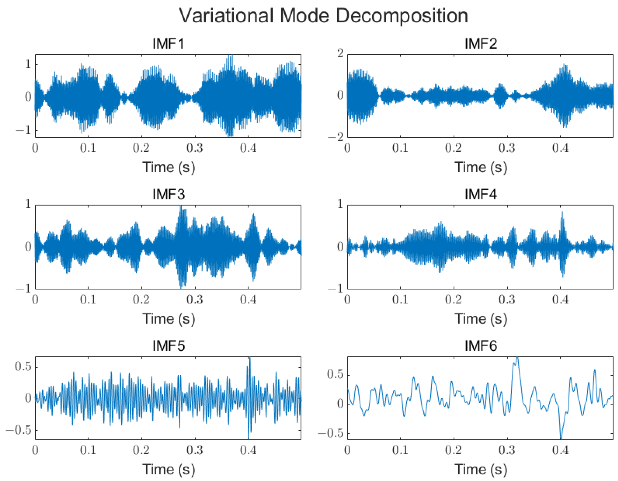
In the experimental phase, the VMD algorithm was applied to the AE signal dataset by substituting the optimal parameters and . The denoising process was executed, and Figure 1 illustrates the plot of intrinsic mode components obtained through the decomposition of a segment of experimentally collected AE signals using the VMD algorithm.
To address the mode components containing noise after decomposition, a comparative experiment was conducted, exploring various threshold functions and different levels of wavelet packet decomposition. After careful evaluation, a hard threshold function, which effectively preserves signal features, was chosen to undergo three-level wavelet packet decomposition on the noisy components, yielding denoised mode components [15]. Subsequently, the denoised mode components were synthesized and reconstructed alongside the retained noise-free mode components to generate the denoised signal. Figure 2 illustrates a comparison with the original AE waveform before and after the denoising process.
As depicted in Figure 2, the VMD algorithm employed in this study showcases remarkable denoising effects. The post-denoising signal waveform exhibits increased stability, effectively eliminating noise while preserving the essential information of the original signal, aligning it seamlessly.
Empirical Mode Decomposition (EMD) is a classic adaptive signal decomposition method that is simple and easy to use, but it may encounter mode mixing issues when dealing with certain complex signals. Improved Complete Ensemble Empirical Mode Decomposition with Adaptive Noise (ICEEMDAN) is an improved version of the Complete Ensemble Empirical Mode Decomposition with Adaptive Noise (CEEMDAN) method, also based on EMD. By introducing noise assistance, ICEEMDAN enhances the stability and reliability of EMD. However, compared to VMD, there may still be limitations in dealing with highly nonlinear and non-stationary signals during the grinding wheel wear process [16]. To quantitatively validate the superiority of the denoising effect of our method, this paper employs the Output Signal-to-Noise Ratio () and Mean Squared Error (MSE) of the denoised signal as metrics. The and MSE of the denoised signals using EMD, ICEEMDAN, and the method employed in this paper are shown in Table 1. Formulas (7) and (8) illustrate the calculation, where n represents the sample quantity, denotes the original signal, and represents the denoised signal.
The obtained by our method was higher than that of EMD and ICEEMDAN denoising, while the MSE was lower than that of EMD and ICEEMDAN. The experimental results indicate that using the VMD method for denoising the AE signals in the grinding wheel grinding process is superior to the denoising effects of EMD and ICEEMDAN, especially in handling highly nonlinear and non-stationary signals. In conclusion, the VMD algorithm utilized in this study was deemed effective in mitigating the noise level of the acoustic emission signal, laying a reliable foundation for subsequent processing by neural network models.
2.2. VMD Algorithm for Denoising AE Signals
2.2.1. Aquila Optimizer
The Aquila Optimizer (AO) algorithm is renowned for its high reliability and consistency, characterized by a robust capability to swiftly converge with strong stability during optimization. The optimization procedure of the Aquila algorithm unfolds through the following steps [17,18].
Step (1): Vertical Dive—Preliminary Determination of Exploration Range.
In this initial step, akin to an eagle soaring high in the sky, the algorithm performs a vertical dive to preliminarily identify the optimal hunting area globally. This step aims to determine the search space wherein the optimal solution is positioned. The corresponding equation is expressed as
In Equation (9), represents the solution for the t iteration of this method; is the best solution, indicating the nearest position of the target prey; t and T represent the current iteration and the maximum iteration times, respectively; represents the mean position of the current solution in the t iteration; ε is a random value between 0 and 1; and is the dimensionality of the problem. N represents the total number of solutions used when computing the mean position in the formula.
Step (2): Short Glide Attack—Narrowing the Exploration Range.
Following the initial identification of the prey area, akin to an eagle hovering above the target prey after soaring from a high altitude, this step involves narrowing down the hunting area. In other words, it aims to reduce the search space of the optimal solution. The corresponding equation is expressed as
In Equations (10)–(13), represents the solution for the t + 1 iteration of this method; is a random solution within [1, N] for the population; x, y are the spiral shapes during the search process; r is the radius during hovering, with taking values from [1, 20]; θ is the hovering angle; U, ω take fixed values 0.00565, 0.005, respectively; takes values from [1, D], where D is the dimension space; L(D) is the hunting flight distribution function; s, β take fixed values 0.01, 1.5, respectively; μ, v take random values within [0, 1]; and Γ is the gamma function. The values and their ranges mentioned above are based on the research method proposed by L. Abualigah et al. in “Aquila Optimizer: A novel meta-heuristic optimization Algorithm” [17].
Step (3): Low-Altitude Flight—Expanding the Exploration Range.
Following the accurate identification of the prey area and when the eagle is prepared to land and attack, this step involves the eagle probing the prey’s reaction in the designated target area through a slow descent and attack mode, gradually approaching the target. The corresponding equation is expressed as
In Equation (14), represents the solution for the t + 1 iteration of this method; α, δ are adjustment parameters, fixed at a small value of 0.1; and and represent the upper and lower bounds of the given problem, respectively.
Step (4): Walking Capture—Narrowing the Exploration Range.
As the eagle closes in on the target, it executes an attack from the air, leveraging the prey’s movement to achieve swift convergence. The corresponding equation is expressed as
In Equation (15), represents the solution for the t + 1 iteration of this method; is the quality function used to balance the search strategy; represents various movements of the eagle in chasing prey; represents the flight slope of the eagle in the hunting process; and X(t) is the current solution for the t iteration.
AO possesses robust global search capabilities, enabling comprehensive exploration of the neural network parameter space to identify the optimal model configuration. Its adaptability allows for adjustments based on the distinct characteristics of the search space, making it suitable for complex tasks related to neural network parameter optimization. AO demonstrates the ability to rapidly converge to a global optimum, proving crucial for enhancing model performance [19]. Whether in terms of model tuning or computational efficiency, AO exhibits favorable performance in the experiments conducted in this paper.
2.2.2. CNN-LSTM
CNN is a type of deep feedforward neural network that relies on convolutional operations, encompassing an input layer, convolutional layer, pooling layer, fully connected layer, and output layer [20]. In this study, the acoustic emission signal’s sample point data is segmented into a one-dimensional dataset, serving as the input data for CNN. Consequently, the convolutional layer utilizes one-dimensional convolution (Conv1D) for computation [21]. Feature extraction in CNN hinges on the convolutional kernels within the convolutional layer. These kernels scan the one-dimensional input data through stepwise translation, performing convolution operations as defined in Equation (16):
In Equation (16), x represents the input layer data; is the i-th convolutional kernel, is the bias of the i-th convolutional kernel; * denotes the convolution operation; and f() is the activation function. In this study, ReLU function was chosen as the activation function, as shown in Equation (17):
LSTM, a refinement of RNN in deep learning, proves to be effective in overcoming the challenge of vanishing gradients encountered in the training process of conventional models. Particularly suited for the analysis and prediction of long-time sequences, LSTM enhances the learning capacity of the network. In contrast to the standard RNN, LSTM introduces a memory state unit in the hidden layer neural nodes to retain past information. It employs three gating structures—namely, the input gate, forget gate, and output gate—to regulate the retention and updating of historical information [22]. Figure 3 illustrates the fundamental unit of LSTM.
The combined prediction model proposed in this paper, CNN-LSTM, is illustrated in Figure 4. In this architecture, CNN performs feature extraction on the aforementioned input layer of AE data, employing two alternating layers of convolutional and pooling layers. The resulting feature vector, denoted as , serves as the input for the LSTM layer. The state memory unit, , is responsible for preserving the motion state information from the preceding time step, while the hidden unit, , records the prediction of the grinding wheel wear state from the previous time step. These three components collectively influence the forget gate, determining which information is to be forgotten. The inputs and undergo transformations through the sigmoid function and tanh function, respectively, jointly influencing the state memory unit to decide which information should be retained. The output gate, , is determined by the updated state memory unit and the output . CNN-LSTM amalgamates the strengths of CNN in capturing local features and LSTM in handling sequential information, rendering it well-suited for processing acoustic emission data. In this study, MSE was selected as the loss function, which is represented as
where n denotes the number of samples, represents the ground truth, and denotes the corresponding predicted value.
In the recognition of grinding wheel wear states, AE signals typically exhibit temporal patterns, and conventional neural network structures struggle to capture this temporal information. CNN can assist in identifying frequency domain features associated with different states during the grinding wheel wear process, capturing detailed information related to wear. LSTM aids in analyzing the temporal aspects of acoustic emission signals. By combining CNN and LSTM, CNN-LSTM can better handle sequential data, possessing stronger spatiotemporal modeling capabilities [23]. Therefore, the combination of CNN-LSTM holds advantages in dealing with the recognition of grinding wheel wear states.
2.2.3. AO-CNN-LSTM Model Design
In this paper, the parameters of the proposed CNN-LSTM combined recognition model undergo optimization using the AO algorithm. Through iterative updates facilitated by the AO algorithm, the objective is to seek optimal network parameters characterized by high accuracy and stability, thereby achieving effective recognition of the grinding wheel wear state. Consequently, a neural network model named AO-CNN-LSTM is formulated.
The key principles governing this neural network model are outlined as follows:
- Define the parameters of the CNN-LSTM model as the optimization objective, specify the population size, and determine the maximum number of iterations for the AO algorithm. Initiate the iterative calculation process.
- Assess based on the iterative conditions, and update the positions of the eagles using the corresponding methods. With each increment in the number of iterations, the positions of individual eagles undergo continuous updates until the termination iteration condition is satisfied, at which point the optimal CNN-LSTM model parameters are output.
- Training the dataset using the optimized AO-CNN-LSTM neural network.
- During the training process, the weights of the CNN-LSTM are updated iteratively based on the trends in Loss and Accuracy using the principles of gradient descent. This strategy ensures the gradual convergence of the predictive model, prevents overfitting, and yields satisfactory accuracy.
- After the iterations cease, the performance of AO-CNN-LSTM is assessed using the test dataset to obtain the optimal model.
3. Experiment
In this section, the relevant instruments and equipment used in the grinding wheel grinding experiment will be introduced, along with the experimental conditions, followed by the calibration of the wear status of the grinding wheel. In Section 3.2, typical AE signals of wear states will be presented, along with the results of denoising the AE signals of typical wear states using VMD. Finally, the dataset collected under experimental conditions will be divided, and the AO-CNN-LSTM model will be used to identify the wear status of the grinding wheel. A comparison and analysis of the classification results and accuracy will be conducted.
3.1. Experimental Conditions
The grinding wheel experiment was conducted on the 3MK1440 high-precision external cylindrical automatic grinding machine, as depicted in Figure 7. The AE detection system employed in the experiment comprises an AE acquisition card, PXR15 AE sensor, PXPA3 preamplifier, and a PC computer. The material of the experimental grinding wheel is ceramic brown corundum, featuring a diameter of 550 mm and a width of 55 mm. The specific experimental grinding parameters encompass a grinding wheel linear velocity of 15 m/s and a grinding feed speed of 100 μm/min. Following the grinding process, a portable surface roughness measuring instrument is employed to assess the surface roughness of the workpiece.
During the grinding experiment, a node was designated for every 500 μm of cumulative grinding, resulting in a total of 10 nodes. Following the grinding completion at each node, the surface morphology of both the grinding wheel and workpiece was carefully observed. The surface roughness of the workpiece after grinding was measured using a portable surface roughness gauge. The wear status of the grinding wheel after completing the grinding at each node was comprehensively analyzed and evaluated by referencing the alterations in the time-domain waveform of the acoustic emission signal.
3.2. Classification and Calibration of Grinding Wheel Wear States
The extent of wear on the grinding wheel has a direct impact on the quality of the workpiece surface grinding. Consequently, surface roughness serves as an indirect indicator reflecting the sharpness and wear condition of the grinding wheel. Throughout the grinding process, abrasive grains continually cut and scrape the workpiece surface, removing material and leaving scratches. As abrasive grains lack a strict arrangement pattern and exhibit a random distribution on the grinding wheel’s surface, grains with varying exposed heights interact with the workpiece simultaneously, resulting in diverse material removal amounts across different regions of the workpiece surface. This randomness leads to the formation of random roughness on the processed workpiece’s surface [24].
Blunted abrasive grains possess weakened cutting performance, unable to effectively remove material to form cutting but instead causing material squeezing on the workpiece surface, resulting in localized elevations. The grinding process induces stress and frictional heat, leading to elastic, plastic deformation, and thermal deformation. This, in turn, contributes to unevenness in height across different regions of the workpiece surface [25].
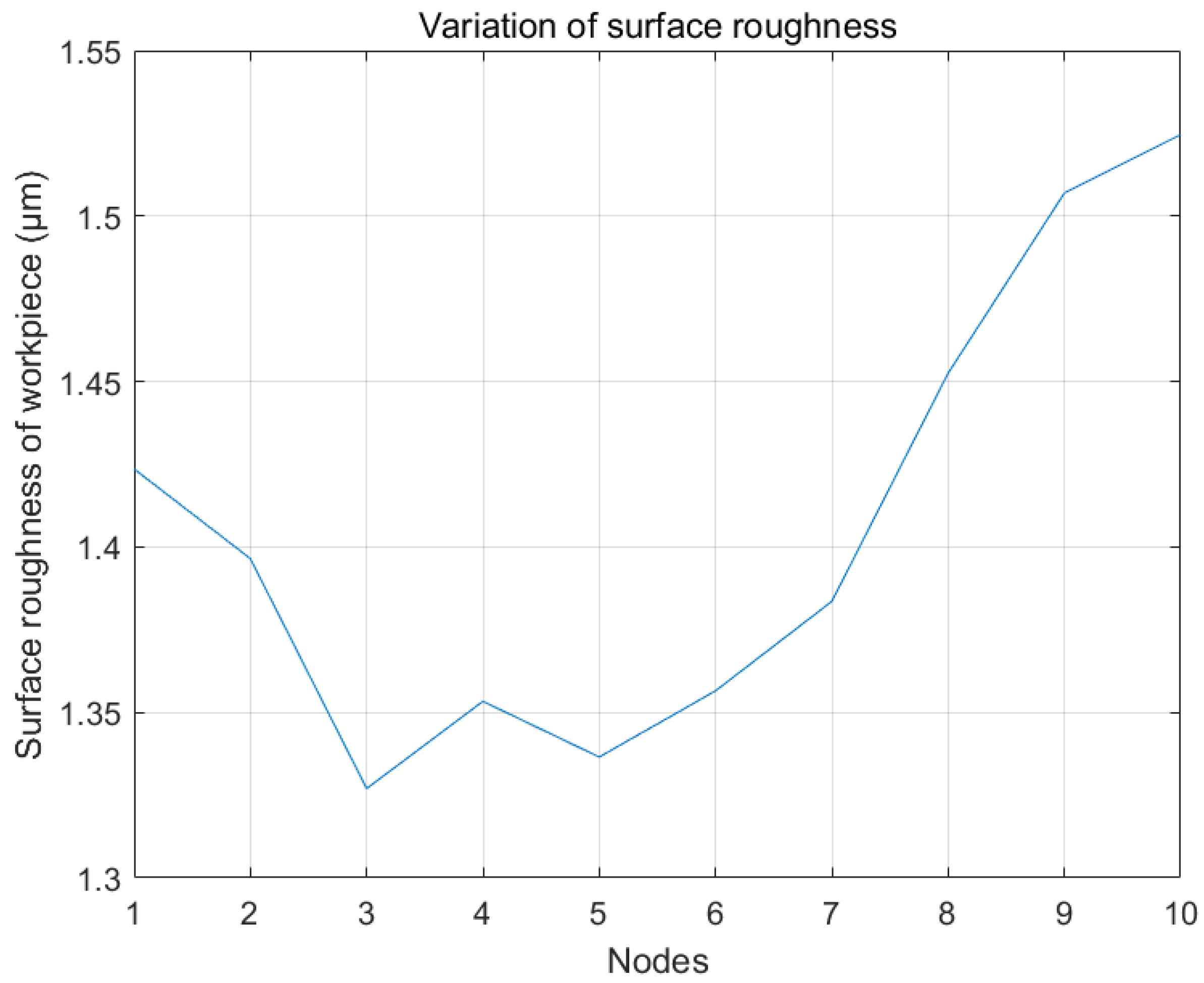
In the grinding experiment conducted in this paper, the variation in surface roughness of the workpiece at each node is illustrated in Figure 8.
The first wear stage corresponds to nodes 1–2, where the surface roughness of the workpiece is relatively low and exhibits a slight decrease. During this stage, the new grinding wheel undergoes initial grinding, and the friction and compression between abrasive grains and the material lead to rapid micro-fracture of these abrasive grains. Additionally, the wear area at the top of some abrasive grains increases. Consequently, the grinding wheel experiences rapid wear in this stage, and the distribution of abrasive grains on the grinding wheel gradually becomes more uniform. Therefore, the removal of material from the workpiece surface is relatively even, resulting in lower surface roughness.
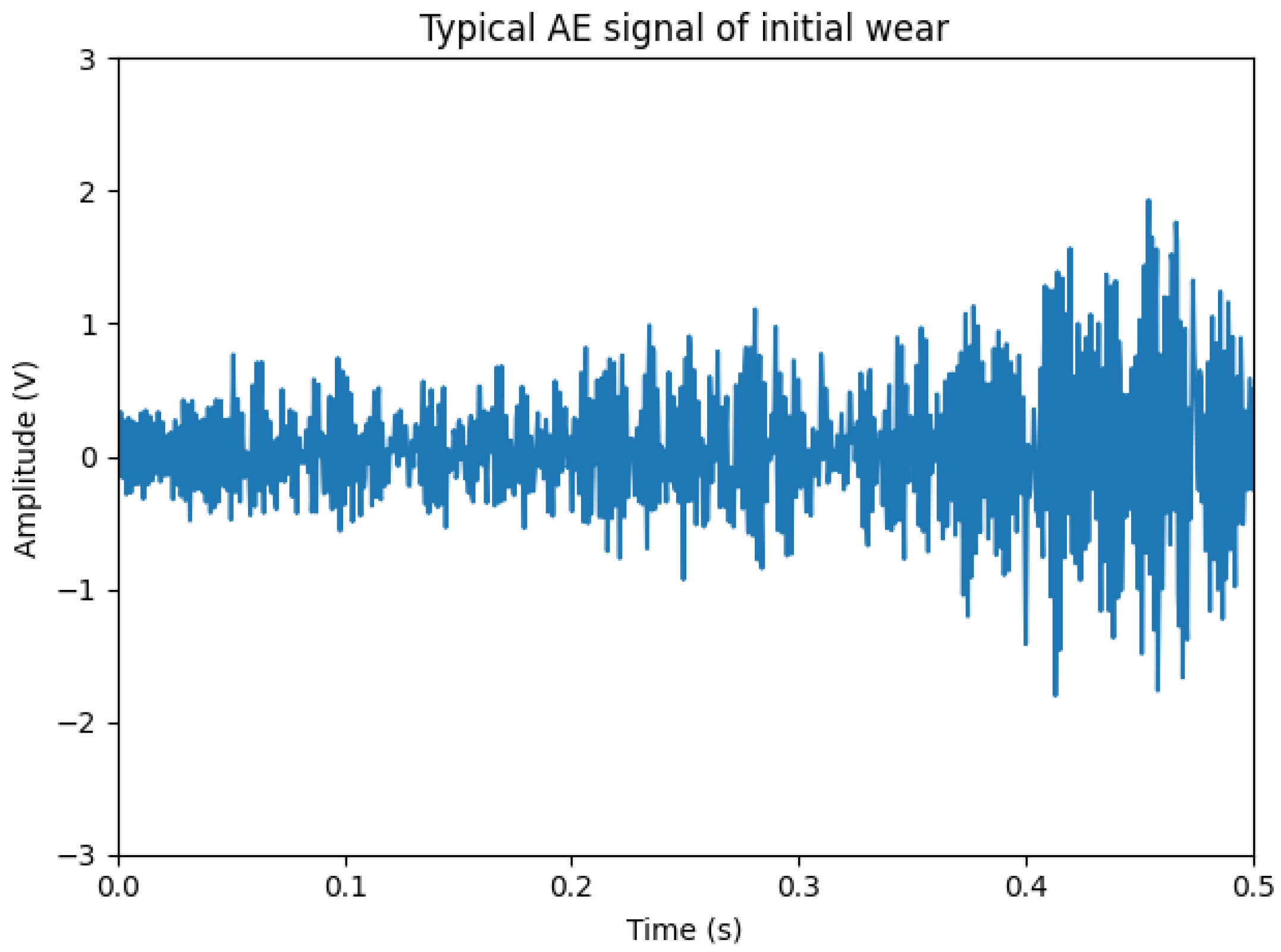
The time-domain waveform of the acoustic emission signal during this stage is depicted in Figure 9, characterized by a relatively small amplitude. Thus, this stage is identified as the initial wear state of the grinding wheel. The result of applying VMD denoising to this typical signal is shown in Figure 10.
The second wear stage corresponds to nodes 3–7, where the surface roughness of the workpiece is relatively low and exhibits a gradual increase. During this wear stage, the wear area at the top of the abrasive grains further expands, and a small portion of the abrasive grains shows signs of fracture or even detachment. Due to the relatively stable condition of the abrasive grains on the grinding wheel during this stage, the amount of wear on the grinding wheel is relatively modest. The grinding performance of the wheel experiences a slight weakening, resulting in a gradual increase in the surface roughness of the workpiece.
The time-domain waveform of the acoustic emission signal during this stage is depicted in Figure 11, featuring a noticeable increase in amplitude that tends to stabilize. Thus, this stage is identified as the intermediate wear state of the grinding wheel. The result of applying VMD denoising to this typical signal is shown in Figure 12.
The third wear stage corresponds to nodes 8–10, where the surface roughness of the workpiece is significantly higher and undergoes a rapid increase. In this wear stage, the wear area at the top of some abrasive grains has become very large, leading to a sharp increase in grinding force and the substantial breakage, fracture, and detachment of numerous abrasive grains. At this juncture, the grinding capability of the wheel severely diminishes, and the contour accuracy of the surface is drastically compromised. The wear rate increases sharply, making it unsuitable for normal grinding, and it should be promptly dressed. During this stage, the grinding performance of the wheel experiences a significant decline, resulting in a rapid increase in the surface roughness of the workpiece.
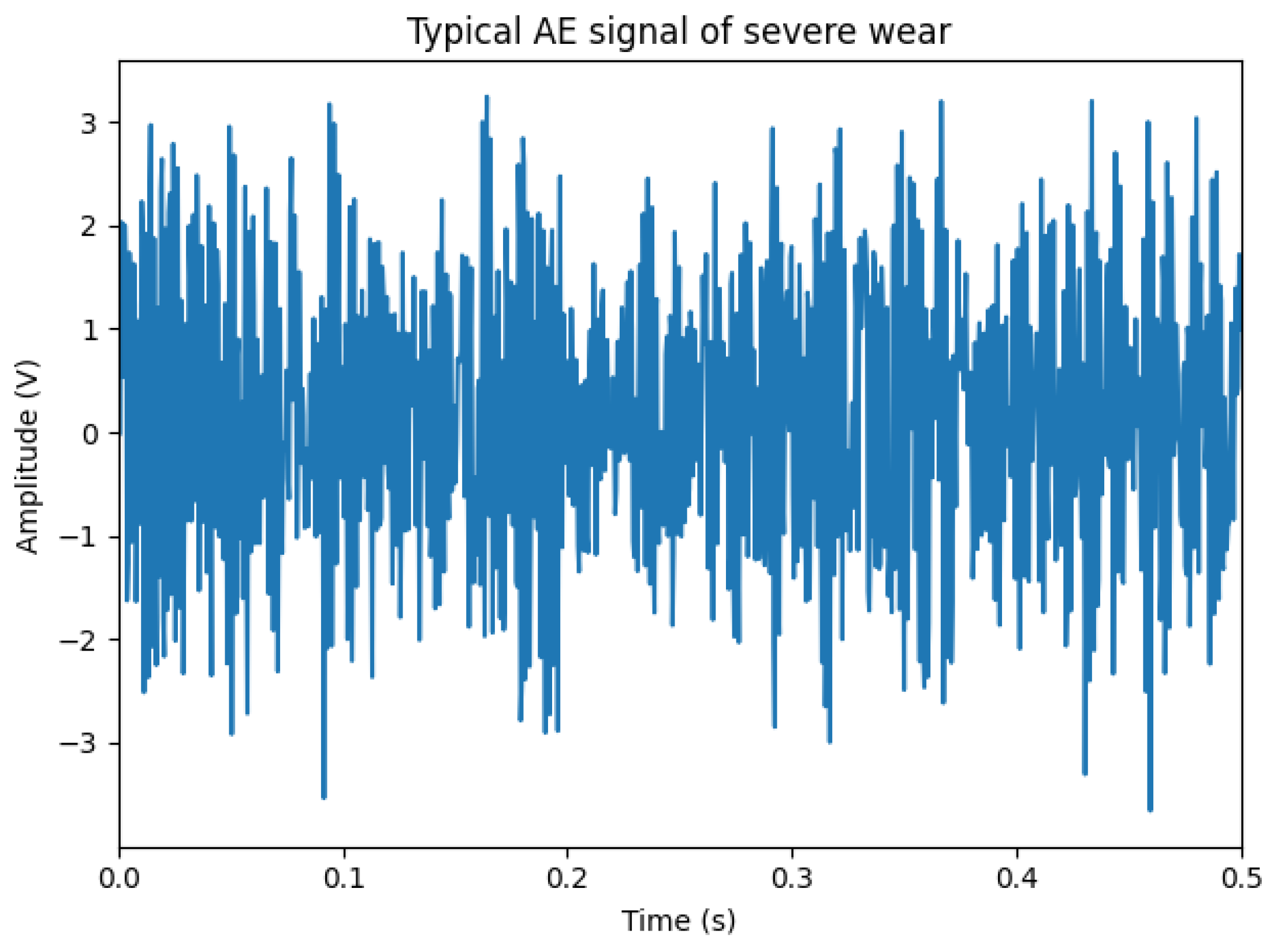
In this stage, the time-domain waveform of the acoustic emission signal is depicted in Figure 13, characterized by an increase in amplitude and significant fluctuations, indicating extreme instability. Therefore, this stage is identified as the severe wear state of the grinding wheel. The result of applying VMD denoising to this typical signal is shown in Figure 14.
3.3. Analysis of VMD Denoising and AO-CNN-LSTM Neural Network Model Recognition Results
Under the experimental conditions outlined in Section 3.1, a total of 8 sets of grinding wheel experiments were conducted in this study. Each experiment involved the collection of 40 segments of AE signals. After initial preprocessing with the PXPA3 preamplifier filter, the signals underwent VMD denoising, resulting in a sample set consisting of 320 segments of AE signals. The grinding wheel wear experiments in this paper are segmented into 10 nodes, and noise-containing datasets are curated by selecting acoustic emission signals from each node. Initially, the Variational Mode Decomposition (VMD) algorithm is employed to denoise the dataset, yielding a sample set. Subsequently, the sample set is partitioned into training, testing, and validation sets. The training and validation sets are harnessed for model training, constituting 70% and 10% of the total sample set, respectively. The testing set is deployed to assess the recognition accuracy of the neural network model for new sample data corresponding to the grinding wheel wear states, constituting 20% of the total sample set. Throughout the experiment, the grinding wheel undergoes three wear states, and one-hot encoding is implemented to assign three sample labels corresponding to the wear states: Initial Wear [1, 0, 0], Intermediate Wear [0, 1, 0], Severe Wear [0, 0, 1] [26]. The labeling and partitioning results of the sample set are presented in Table 2.
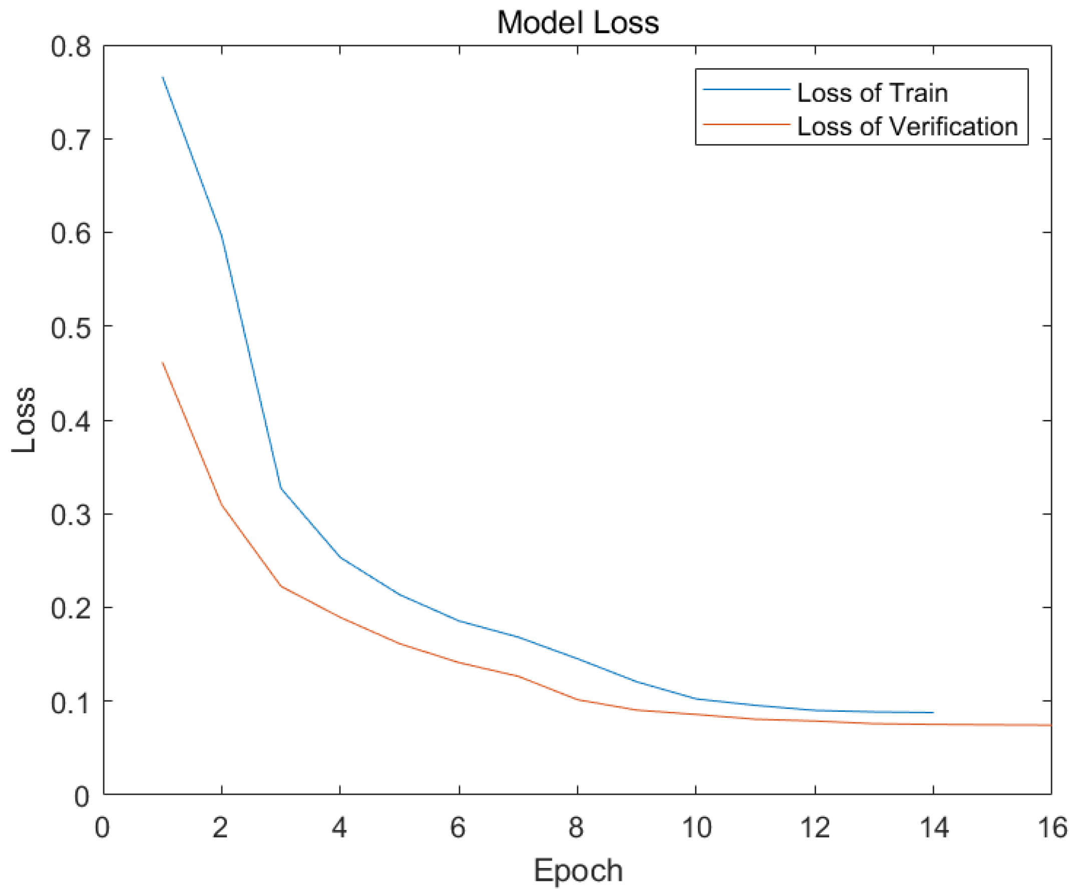
To intuitively assess the overall performance of the proposed grinding wheel wear recognition model in this study, three metrics were employed: the loss curve, and the accuracy by using the confusion matrix to compare the true category and the predicted category.
The loss function during training is illustrated in Figure 15. It can be observed that the loss function rapidly decreases in the early stages of training, and as the number of training iterations increases, the rate of decline gradually slows down, ultimately reaching a stable state. The trend indicates that the model training converges, demonstrating effective training results.
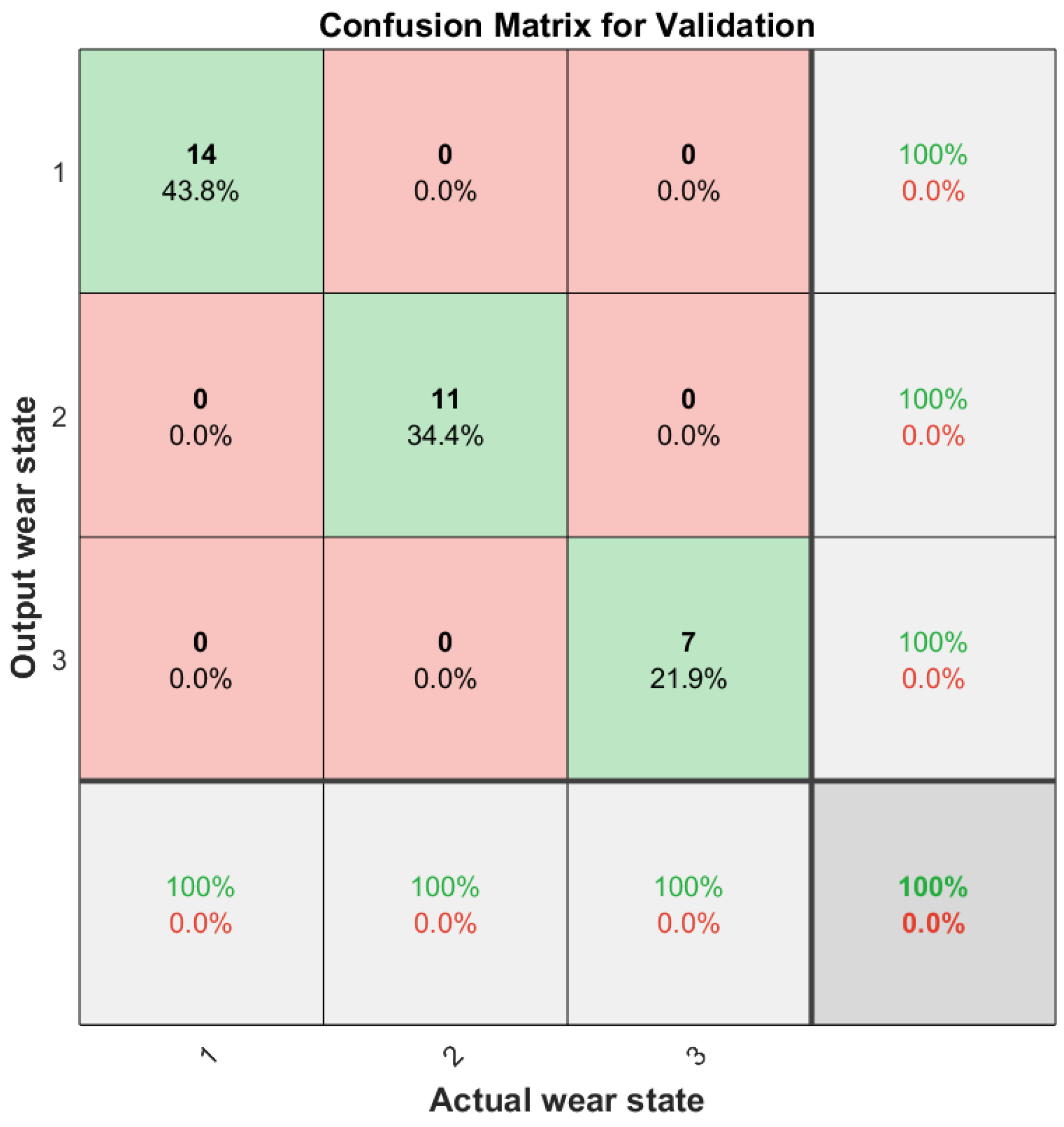
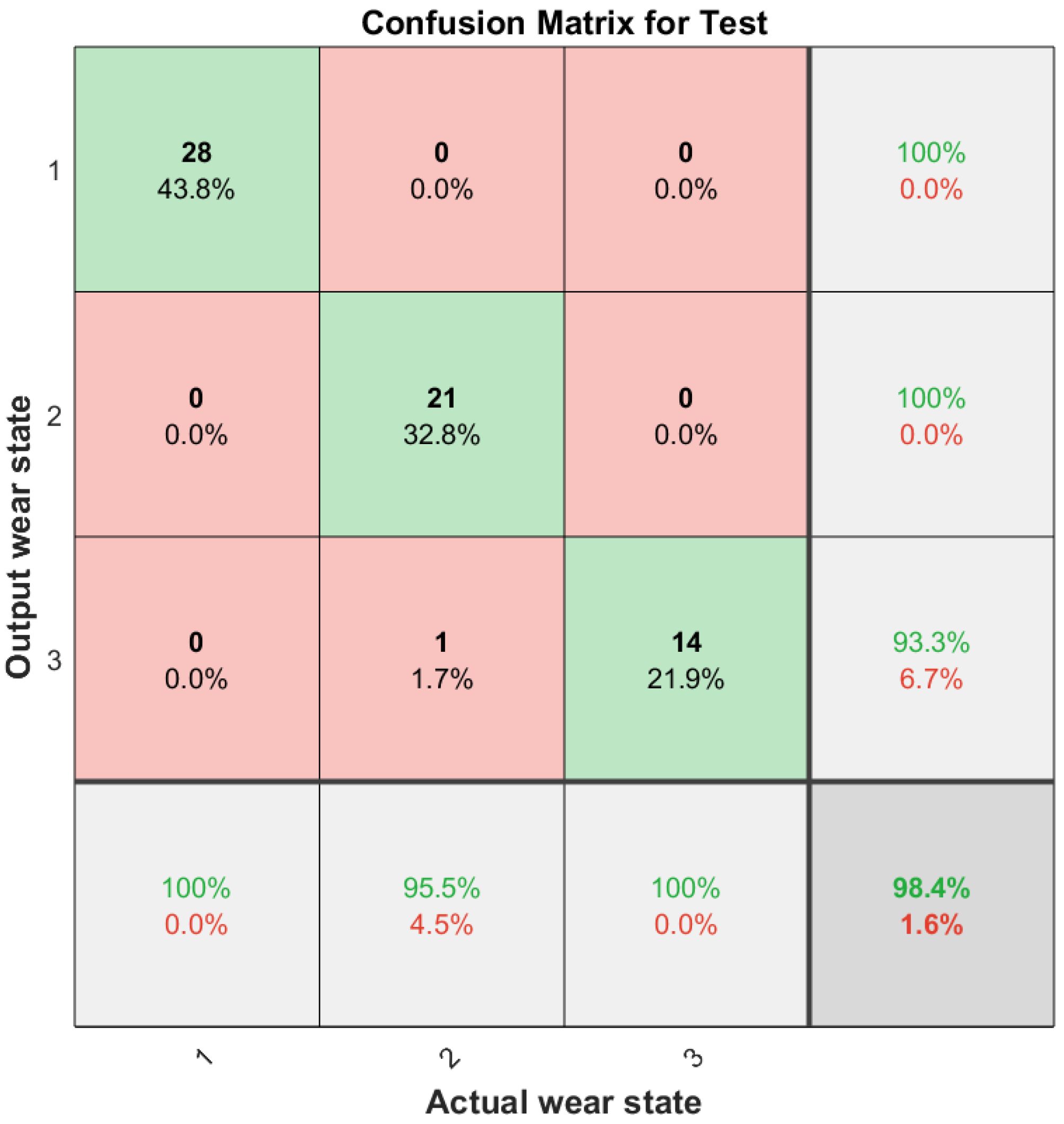
Accuracy refers to the proportion of correctly classified samples among the total number of samples. The confusion matrix summarizes dataset records in a matrix form based on two criteria: the true category and the predicted category by the classification model. The rows of the matrix represent the true values, while the columns represent the predicted values [27]. The classification accuracy on the training set, validation set, and test set, along with the overall classification confusion matrix, is illustrated in Figure 16, Figure 17, Figure 18 and Figure 19, where 1 represents Initial Wear, 2 represents Intermediate Wear, and 3 represents Severe Wear. In the confusion matrix, green represents correct classification, while red represents misclassification.
The confusion matrix clearly demonstrates the classification performance of the model proposed in this paper on the grinding wheel wear dataset. The overall precision and recall of the model are both above 95%, showing high comprehensive performance. The precision of the model for all three categories exceeds 95%, with the precision of initial wear and intermediate wear both exceeding 99%, resulting in an overall recognition accuracy of 98.8%. The recall rate of the model for severe wear is 100%, indicating that the model successfully captures and identifies all samples truly belonging to this category without missing any. Observing the off-diagonal areas of the confusion matrix, it can be noted that the values in these areas are small, indicating a low probability of misclassification by the model proposed in this paper. These characteristics demonstrate that the proposed model exhibits good discriminative ability in processing the acoustic emission signals during the grinding wheel wear process, enabling better capture of grinding wheel wear characteristics.
Furthermore, for comparison, this paper also employs a CNN neural network model for classifying grinding wheel wear states, with the confusion matrix shown in Figure 20. As can be seen from the figure, the recognition accuracy of CNN is lower, at 89%. This indicates that a single CNN tends to overlook temporal information when processing time-series data, limiting its effectiveness in grinding wheel wear identification. This also serves as evidence highlighting the superiority of the algorithm proposed in this paper in the field of grinding wheel wear state recognition.
4. Conclusions
This paper proposes a novel approach for grinding wheel wear recognition based on VMD denoising and the AO-CNN-LSTM algorithm, aiming to improve the recognition rate of different wear states of grinding wheels in noisy environments. Drawing on previous research experience, the variation in AE signals is crucial for determining the grinding wheel wear state. Therefore, this study employs the method of VMD decomposition combined with wavelet denoising reconstruction, which proves effective in handling AE in noisy environments, making the dataset more reliable. For feature extraction and processing, this paper utilizes the CNN-LSTM architecture based on AO-optimized parameters. The experimental results indicate that the method achieves an overall recognition accuracy of 98.8%, with precision rates exceeding 99% for both initial wear and intermediate wear classifications, and a recall rate of 100% for severe wear. In future research, we will continue to collect more wear data from different grinding conditions and different types of grinding wheels, aiming to enhance the efficiency of AE signal processing and improve the universality of the grinding wheel wear recognition model. The main contributions of this study are highlighted as follows:
- The paper successfully introduces a new method based on AE, signal processing, and deep learning, effectively identifying grinding wheel wear states.
- The VMD denoising method in this paper significantly reduces the impact of noise on AE, enhancing the effectiveness of the sample dataset.
- The comprehensive neural network AO-CNN-LSTM, combining CNN and LSTM, with the introduction of AO-optimized parameters. This neural network, when processing AE signals during grinding wheel abrasion, is more adept at capturing temporal information than traditional neural networks, exhibiting stronger spatiotemporal modeling capabilities.
- AO enhances the global search capabilities of neural network parameter optimization, aiding in finding optimal model configurations. Its robust adaptability and convergence speed further enhance recognition accuracy. This study provides valuable insights into the combination of AO with various deep learning architectures.
Author Contributions
Conceptualization, K.X.; methodology, K.X. and D.F.; software, D.F.; validation, K.X.; formal analysis, K.X. and D.F.; investigation, D.F.; resources, K.X.; data curation, K.X.; writing—original draft preparation, D.F.; writing—review and editing, K.X. and D.F.; visualization, D.F.; supervision, K.X.; project administration, K.X.; funding acquisition, K.X. All authors have read and agreed to the published version of the manuscript.
Funding
This research was funded by the National Natural Science Foundation of China, grant number 52275054, 51205108 and 51575161.
Institutional Review Board Statement
Not applicable.
Informed Consent Statement
Not applicable.
Data Availability Statement
The datasets presented in this article are not readily available because the data are part of an ongoing study.
Acknowledgments
The authors wish to thank Henan University of Science and Technology for their assistance and support with this research.
Conflicts of Interest
The authors declare no conflicts of interest.
References
- Novoselov, Y.; Bratan, S.; Bogutsky, V. Analysis of Relation between Grinding Wheel Wear and Abrasive Grains Wear. Procedia Eng. 2016, 150, 809–814. [Google Scholar] [CrossRef]
- Lezanski, P. An intelligent system for grinding wheel condition monitoring. J. Am. Acad. Dermatol. 2001, 109, 258–263. [Google Scholar] [CrossRef]
- Huang, W.; Li, Y.; Wu, X.; Shen, J. The wear detection of mill-grinding tool based on acoustic emission sensor. Int. J. Adv. Manuf. Technol. 2023, 124, 4121–4130. [Google Scholar] [CrossRef]
- Lin, Y.-K.; Wu, B.-F.; Chen, C.-M. Characterization of Grinding Wheel Condition by Acoustic Emission Signals’. In Proceedings of the 2018 International Conference on System Science and Engineering (ICSSE), New Taipei City, Taiwan, 28–30 June 2018; pp. 1–6. [Google Scholar]
- Yang, Z.; Yu, Z. Grinding wheel wear monitoring based on wavelet analysis and support vector machine. Int. J. Adv. Manuf. Technol. 2012, 62, 107–121. [Google Scholar] [CrossRef]
- Mahata, S.; Shakya, P.; Babu, N.R. A robust condition monitoring methodology for grinding wheel wear identification using Hilbert Huang transform. Precis. Eng. 2021, 70, 77–91. [Google Scholar] [CrossRef]
- González, D.; Alvarez, J.; Sánchez, J.A.; Godino, L.; Pombo, I. Deep Learning-Based Feature Extraction of Acoustic Emission Signals for Monitoring Wear of Grinding Wheels. Sensors 2022, 22, 6911. [Google Scholar] [CrossRef] [PubMed]
- Bi, G.; Liu, S.; Su, S.; Wang, Z. Diamond Grinding Wheel Condition Monitoring Based on Acoustic Emission Signals. Sensors 2021, 21, 1054. [Google Scholar] [CrossRef]
- Lee, C.-H.; Jwo, J.-S.; Hsieh, H.-Y.; Lin, C.-S. An Intelligent System for Grinding Wheel Condition Monitoring Based on Machining Sound and Deep Learning. IEEE Access 2020, 8, 58279–58289. [Google Scholar] [CrossRef]
- Avci, O.; Abdeljaber, O.; Kiranyaz, S.; Hussein, M.; Gabbouj, M.; Inman, D.J. A review of vibration-based damage detection in civil structures: From traditional methods to Machine Learning and Deep Learning applications. Mech. Syst. Signal Process. 2021, 147, 107077. [Google Scholar] [CrossRef]
- Li, H.; Liu, T.; Wu, X.; Chen, Q. An optimized VMD method and its applications in bearing fault diagnosis. Measurement 2020, 166, 108185. [Google Scholar] [CrossRef]
- Rout, S.K.; Biswal, P.K. An efficient error-minimized random vector functional link network for epileptic seizure classification using VMD. Biomed. Signal Process. Control. 2020, 57, 101787. [Google Scholar] [CrossRef]
- Dragomiretskiy, K.; Zosso, D. Variational Mode Decomposition. IEEE Trans. Signal Process. 2014, 62, 531–544. [Google Scholar] [CrossRef]
- Wang, Y.; Liu, F.; Jiang, Z.; He, S.; Mo, Q. Complex variational mode decomposition for signal processing applications. Mech. Syst. Signal Process. 2017, 86, 75–85. [Google Scholar] [CrossRef]
- Lorraine, K.J.S.; Ramarakula, M. An efficient interference mitigation approach for NavIC receivers using improved variational mode decomposition and wavelet packet decomposition. Trans. Emerg. Telecommun. Technol. 2021, 32, e4242. [Google Scholar] [CrossRef]
- Elouaham, S.; Dliou, A.; Elkamoun, N.; Latif, R.; Said, S.; Zougagh, H.; Khadiri, K. Denoising electromyogram and electroencephalogram signals using improved complete ensemble empirical mode decomposition with adaptive noise. Indones. J. Electr. Eng. Comput. Sci. 2021, 23, 829–836. [Google Scholar] [CrossRef]
- Abualigah, L.; Yousri, D.; Elaziz, M.A.; Ewees, A.A.; Al-Qaness, M.A.; Gandomi, A.H. Aquila Optimizer: A novel meta-heuristic optimization algorithm. Comput. Ind. Eng. 2021, 157, 107250. [Google Scholar] [CrossRef]
- Fatani, A.; Dahou, A.; Al-Qaness, M.A.A.; Lu, S.; Elaziz, M.A. Advanced Feature Extraction and Selection Approach Using Deep Learning and Aquila Optimizer for IoT Intrusion Detection System. Sensors 2022, 22, 140. [Google Scholar] [CrossRef]
- Verma, M.; Sreejeth, M.; Singh, M.; Babu, T.S.; Alhelou, H.H. Chaotic Mapping Based Advanced Aquila Optimizer With Single Stage Evolutionary Algorithm. IEEE Access 2022, 10, 89153–89169. [Google Scholar] [CrossRef]
- Bhatt, D.; Patel, C.; Talsania, H.; Patel, J.; Vaghela, R.; Pandya, S.; Modi, K.; Ghayvat, H. CNN Variants for Computer Vision: History, Architecture, Application, Challenges and Future Scope. Electronics 2021, 10, 2470. [Google Scholar] [CrossRef]
- Surinta, O. Deep feature extraction technique based on Conv1D and LSTM network for food image recognition. Eng. Appl. Sci. Res. 2021, 48, 581592. [Google Scholar] [CrossRef]
- DiPietro, R.; Hager, G.D. Chapter 21—Deep learning: RNNs and LSTM. In Handbook of Medical Image Computing and Computer Assisted Intervention; Zhou, S.K., Rueckert, D., Fichtinger, G., Eds.; The Elsevier and MICCAI Society Book Series; Academic Press: Cambridge, MA, USA, 2020; pp. 503–519. [Google Scholar] [CrossRef]
- Ozcanli, A.K.; Baysal, M. Islanding detection in microgrid using deep learning based on 1D CNN and CNN-LSTM networks. Sustain. Energy Grids Netw. 2022, 32, 100839. [Google Scholar] [CrossRef]
- Yin, G.; Guan, Y.; Wang, J.; Zhou, Y.; Chen, Y. Multi-information fusion recognition model and experimental study of grinding wheel wear status. Int. J. Adv. Manuf. Technol. 2022, 121, 3477–3498. [Google Scholar] [CrossRef]
- Yin, G.; Wang, J.; Guan, Y.; Wang, D.; Sun, Y. The prediction model and experimental research of grinding surface roughness based on AE signal. Int. J. Adv. Manuf. Technol. 2022, 120, 6693–6705. [Google Scholar] [CrossRef]
- Seger, C. An Investigation of Categorical Variable Encoding Techniques in Machine Learning: Binary versus One-Hot and Feature Hashing. 2018. Available online: https://urn.kb.se/resolve?urn=urn:nbn:se:kth:diva-237426 (accessed on 28 January 2024).
- Zeng, G. On the confusion matrix in credit scoring and its analytical properties. Commun. Stat.-Theory Methods 2019, 49, 2080–2093. [Google Scholar] [CrossRef]
Figure 1.
IMFs after VMD.

Figure 2.
Waveform comparison before and after VMD-wavelet denoising.

Figure 3.
Basic unit of LSTM.

Figure 4.
The structure of the CNN-LSTM model.

Figure 5.
Flowchart of optimizing neural network parameters using AO.

Figure 6.
Flowchart of the AO-CNN-LSTM.

Figure 7.
Grinding Wheel Experiment Workbench.

Figure 8.
Surface roughness variation of the workpiece at each node.

Figure 9.
Typical AE signal of initial wear.

Figure 10.
Typical AE signal of initial wear after VMD denoising.

Figure 11.
Typical AE signal of intermediate wear.

Figure 12.
Typical AE signal of intermediate wear after VMD denoising.

Figure 13.
Typical AE signal of severe wear.

Figure 14.
Typical AE signal of severe wear after VMD denoising.

Figure 15.
The Loss function of Train set and Validation set during training.

Figure 16.
Confusion Matrix for Train.

Figure 17.
Confusion Matrix for Validation.

Figure 18.
Confusion Matrix for Test.

Figure 19.
Confusion Matrix for Sample.

Figure 20.
Confusion Matrix for CNN.


Table 1.
The signal denoising indicators of different denoising methods.
| Denoising Methods | MSE | |
|---|---|---|
| EMD | 7.69 | 0.0723 |
| ICEEMDAN | 9.15 | 0.0092 |
| Our method | 10.34 | 0.0081 |
Table 2.
Labeling and Partitioning of the Sample Set.
| Sample Correspondences with Grinding Wheel Wear States | Initial Wear | Intermediate Wear | Severe Wear | |
|---|---|---|---|---|
| Sample labels | [1, 0, 0] | [0, 1, 0] | [0, 0, 1] | |
| Sample quantities | Training set | 99 | 75 | 50 |
| Validation set | 14 | 11 | 7 | |
| Test set | 28 | 22 | 14 | |
Disclaimer/Publisher’s Note: The statements, opinions and data contained in all publications are solely those of the individual author(s) and contributor(s) and not of MDPI and/or the editor(s). MDPI and/or the editor(s) disclaim responsibility for any injury to people or property resulting from any ideas, methods, instructions or products referred to in the content. |
© 2024 by the authors. Licensee MDPI, Basel, Switzerland. This article is an open access article distributed under the terms and conditions of the Creative Commons Attribution (CC BY) license (https://creativecommons.org/licenses/by/4.0/).
Share and Cite
MDPI and ACS Style
Xu, K.; Feng, D. A Method for Identifying the Wear State of Grinding Wheels Based on VMD Denoising and AO-CNN-LSTM. Appl. Sci. 2024, 14, 3554. https://doi.org/10.3390/app14093554
AMA Style
Xu K, Feng D. A Method for Identifying the Wear State of Grinding Wheels Based on VMD Denoising and AO-CNN-LSTM. Applied Sciences. 2024; 14(9):3554. https://doi.org/10.3390/app14093554
Chicago/Turabian StyleXu, Kai, and Dinglu Feng. 2024. "A Method for Identifying the Wear State of Grinding Wheels Based on VMD Denoising and AO-CNN-LSTM" Applied Sciences 14, no. 9: 3554. https://doi.org/10.3390/app14093554
Note that from the first issue of 2016, this journal uses article numbers instead of page numbers. See further details here.