
Numerical Simulation of a Submerged Floating Tunnel: Validation and Analysis
1
Institute of Geophysics, China Earthquake Administration, Beijing 100081, China
2
Department of Civil Engineering, Tsinghua University, Beijing 100084, China
*
Author to whom correspondence should be addressed.
Appl. Sci. 2024, 14(9), 3589; https://doi.org/10.3390/app14093589
Submission received: 1 March 2024
/
Revised: 8 April 2024
/
Accepted: 22 April 2024
/
Published: 24 April 2024
(This article belongs to the Special Issue Seismic Analysis and Design of Ocean and Underground Structures)
Abstract
:The dynamic response analysis of submerged floating tunnels (SFTs) under seismic action is a complex two-way fluid–structure coupling problem that requires expertise in structural dynamics, fluid mechanics, and advanced computational methods. The coupled Eulerian–Lagrangian (CEL) method is a promising method for solving fluid–structure interaction problems, but its application to SFTs is not well established. Therefore, it is crucial to verify the accuracy and reliability of the CEL method in fluid–structure coupling simulations. This study verified the applicability of the CEL method for simulating one-way and two-way fluid–structure coupling cylindrical flow problems, and then applied the CEL method for the analysis of a shaking table test of a model SFT. A comparison of results obtained with the CEL method with those obtained in a previous indoor model test of an SFT demonstrates the agreement between the results of the CEL method and the overall trend of the experimental results, indicating the reliability of the method for the seismic analysis of SFTs. Moreover, the analysis of the dynamic response characteristics of SFTs under seismic conditions provides data support and a technological means for the seismic design of SFTs.
1. Introduction
Submerged floating tunnels (SFTs), which consist of a tubular structure supported by its buoyancy and anchored to two banks via anchor cables and foundations, offer outstanding environmental and economic prospects as transportation structures. However, despite the increasing research attention paid to SFTs, none have been built anywhere in the world. Moreover, SFTs were listed as one of the 60 major engineering technology problems at the 2018 Annual Meeting of the Chinese Association of Science and Technology [1].
Scholars in China and other countries have extensively studied the dynamic responses of SFT structures under seismic action, the vibration characteristics of tethered anchor structures, and the worst-affected response areas of SFT structures. For instance, Wu et al. [2] analyzed the dynamic response of SFTs under combined wave flow–earthquake action through scaled-down model tests and numerical simulations. They concluded that the dynamic response of SFTs under the action of waves and flow alone is relatively small, but that the effect of seismic loading dominates under the combined action of earthquakes and wave flow, and that the flow can attenuate the effects of high-frequency earthquake motions on SFTs. Li et al. [3] used the finite-element method to analyze the static and dynamic responses of a tension-leg SFT. They found that the seismic dynamic response of the SFT could be approximated as the superposition of the two following parts: the dynamic water pressure generated by a seismic wave propagating through seawater, and the additional external force induced by the offset of the submarine support. Their calculation results showed that the weak links were the two ends of the tube body, which were embedded in the rock layer and at the cable location, respectively. Therefore, special attention needs to be paid to these areas during the design process. Xiang et al. [4] believes that, due to the absence of comprehensive analysis methods and calculation procedures for SFTs under seismic and wave forces, it is crucial to establish a multi-scale theoretical model and conduct the corresponding experimental studies. This will facilitate obtaining more precise analysis results and verifying the effectiveness of various seismic protection measures. Wu et al. [5] believes that the ratio of parametric frequency to natural frequency, the direction and magnitude of earthquake excitation, the initial tension in the cable, and the damping ratio all have significant influences on the hydrodynamic and seismic responses of the cable. Therefore, these effects must be considered rigorously during the design of anchor systems for submerged floating tunnels. Fogazzi [6] devised a calculation method that considers the mutual coupling between a fluid, a structure, an anchor foundation, and soil, and an anchor’s geometric nonlinearity when determining the seismic response of anchored SFTs. Martinelli et al. [7,8] have devised a new method for obtaining a response spectrum based on the median pseudo-acceleration spectrum and demonstrated its suitability for SFT engineering design calculations. Brancaleoni et al. [9] derived an equation for calculating the dynamic response of an SFT under seismic and wave effects that can be applied to both short-span SFTs with anchorages and long-span SFTs with underwater piers. Martire et al. [10] examined the seismic response characteristics of SFTs under multi-point support excitation, and they found that it excites more vibration modes in SFTs with longer spans than in SFTs with shorter spans. Xiao et al. [11] considered various simple boundary conditions (such as hinged, solid, and elastic supports) for the SFT with a channel barge structure and showed that a support with the appropriate elastic stiffness can significantly reduce seismic effects on an SFT structure. Chen et al. [12] found that the dynamic response of SFTs to seismic traveling waves is significant, with the most unfavorable response site being the connection between an SFT and its bank foundation. Chao and Xiang [13,14] proposed an anchor-displacement calculation method that integrates along the height of the SFT by parts, which demonstrated the advantages of simplicity and feasibility. Sun and Chen [15,16,17,18] have conducted the first experimental studies of a scaled-down model of an SFT under seismic conditions using an underwater shaking table, which revealed that horizontal seismic excitation could cause the horizontal rotation of an SFT tube. Additionally, the seismic response under an anchor cable inclination angle of 45° was less than that under an anchor cable inclination angle of 60°.
As described above, there have been detailed studies of SFTs under seismic conditions, based on the models and numerical calculations of coupling between SFTs’ tubes and support systems, and the fluids in which they are submerged. These studies have focused on various aspects of SFTs, such as their dynamic responses, how they are affected by fluid forces, and the dynamic characteristics of anchor cables. The calculation methods and research results generated from these studies have significantly contributed to the successful implementation and completion of future SFT projects.
Scaled-down model tests of SFTs serve as a crucial means for understanding the force characteristics of SFTs’ structural systems. However, due to the complex water environment surrounding SFTs, it is challenging to model prototypical structures with perfect fidelity, so satisfactory test results often cannot be obtained. There are three primary challenges. First, SFT model testing is performed on a model consisting of a tunnel body, an anchor cable, and a soil body, and therefore requires the use of multiple materials, and it is difficult to maintain physical similarity between model materials and a prototype. Second, it is challenging to accurately replicate a prototype structure’s detailed characteristics in a large-scale model, which hinders large-scale model testing. Third, calculating the dynamic boundary effects of the scaled-down model system requires the refinement of the model test results via fast and efficient numerical simulation techniques.
The application of the CEL method in the calculation of hydrodynamic loads significantly overcomes some limitations of traditional methods. Conventional methods Huaqing Zhang and Zhiwen Yang [19] for calculating hydrodynamic loads typically assume that underwater structures are fixed to obtain external hydrodynamic loads. Then, using the known hydrodynamic loads, they calculate the structural response. For instance, the Morrison equation [20] assumes that the structure is stationary, while, in reality, the submerged floating tunnel undergoes certain relative displacements under the influence of hydrodynamic loads. This phenomenon is often challenging to accurately simulate using traditional methods.
In the case of employing the CEL method, we can more precisely consider the interaction between the submerged floating tunnels and the surrounding water, achieving bidirectional fluid–structure coupling calculations. Compared to traditional methods like the Morrison equation, the CEL method is more in line with reality because it thoroughly considers the potential relative displacements of underwater structures under hydrodynamic loads. This characteristic enables the CEL method to provide more accurate and realistic numerical results, offering a more reliable basis for engineering designs and structural response analysis.
Therefore, by adopting the CEL method, we not only address the limitations of traditional methods in considering structural displacements, but we also simulate hydrodynamic loads in conditions closer to real-world scenarios. This advantage highlights the significant innovation and practicality of the CEL method in underwater structure research.
In recent years, new numerical calculation methods (such as the smoothed particle hydrodynamics method, the arbitrary Lagrangian–Eulerian method, and the volume of fluid method) have provided powerful technical support for solving complex fluid–structure coupling problems relevant to SFTs. At present, few scholars have used the CEL method for the seismic response analysis of SFT. This paper reports the first attempt to adopt the coupled Eulerian–Lagrangian (CEL) method to conduct the seismic response analysis of an SFT.
2. CEL Method for One- and Two-Way Fluid–Structure Coupling Validation
2.1. CEL Method
Lagrangian methods are widely used for static analysis in geotechnical and structural engineering. Matsui and San [21] simulated slope stability problems, and Shiau et al. [22] analyzed the ultimate bearing capacity of sandy soil foundations based on the limit analysis method. In the Lagrangian method, the cell grid is unified with the object to be analyzed. Thus, during calculation, the shape of the analyzed object remains the same, while that of the finite element mesh changes, and the material does not flow from cell to cell.
In contrast, the Eulerian method is characterized by a fixed finite element mesh in terms of shape, size, and spatial location throughout the numerical computation. Material can flow between the mesh and the grid, so the method is ideal for dealing with material distortion and certain large deformation problems [23]. However, the Eulerian method struggles to accurately capture boundary information about the objects and materials, and so is typically used in the computational analysis of fluid dynamics.
Pure Lagrangian and pure Eulerian methods each have strengths and weaknesses, and by combining these methods, it is possible to take advantage of their strengths while overcoming their weaknesses. The CEL method was devised by Noh [24] for this purpose, and has since been used in fluid–solid coupling analysis, where the Lagrangian mesh is used to discretize the solid, whereas the Eulerian mesh is used to discretize the fluid domain. The Lagrangian mesh can pass through the fluid domain formed by the Eulerian mesh, thereby defining the contact between the fluid and solid materials. The CEL method has also been used to numerically simulate a variety of phenomena, including the scouring of vertical breakwaters [25] and a steel water-storage tank under blast loading [26], and has been employed for the development of a Reynolds-averaged Eulerian–Lagrangian model of vortex interaction that simulates the turbulent suspension of flow in a thin plate [27].
Specifically, the basic idea of the CEL method is to divide the computational domain into small Eulerian regions, with the physical quantities within each Eulerian region being described by a Lagrangian function. During the time-stepping process, the physical quantities within the Eulerian regions are first calculated, and then these quantities are transferred to the adjacent Eulerian regions through interpolation, forming a complete Lagrangian description of the computational domain. Therefore, the CEL method can control the accuracy of different spatial scales through multi-level grids, and can adapt to different physical processes via the use of different time steps.
The calculation process of the CEL method includes the following steps:
- (1)
- Partitioning Eulerian regions: Divide the computational domain into several small Eulerian regions.
- (2)
- Constructing Lagrangian functions: For each physical quantity within each Eulerian region, construct a corresponding Lagrangian function.
- (3)
- Solving Euler equations: For each physical quantity within each Eulerian region, use the Euler method to solve its corresponding Euler equation.
- (4)
- Interpolation transfer: Use interpolation methods to transfer physical quantities within Eulerian regions to adjacent Eulerian regions, forming a complete Lagrangian description of the computational domain.
- (5)
- Time stepping: Repeat steps 3 and 4 to perform time-stepping calculations.
2.1.1. Fluid Motion Equations (Eulerian Equations)
The Eulerian equations describe the motion of the fluid, typically in the form of the Navier–Stokes equations. For incompressible fluids, the Navier–Stokes equations [24] can be written as
Momentum conservation equation:
Here, is the density, is the velocity vector, is the dynamic viscosity coefficient, is the velocity gradient, represents the static pressure, and is the gravitational acceleration vector.
2.1.2. Solid Motion Equations (Lagrangian Equations)
In the Lagrangian coordinate system, the motion of the solid is typically described using elastic mechanics or other solid dynamics models (Noh, 1964). The basic equation for solid motion can be written as
Motion equation:
Here, is the density of the solid, is the displacement vector of the solid, is the elastic modulus, and is the gravitational vector.
2.1.3. Coupling
As mentioned above, in the CEL (coupled Eulerian-Lagrangian) method, there exist motion equations in two different coordinate systems (Eulerian and Lagrangian). A common strategy to tackle this issue in coupling methods involves introducing interface coupling conditions to coordinate the exchange of information between the two systems. These interface conditions may encompass characterizing the forces exerted by the fluid on the solid and the influence of the solid on the fluid in terms of forces and displacements. By using the CEL method, the contact between the Eulerian domain and Lagrangian domain is discretized using the general contact algorithm, which is based on the penalty contact method [28]. The penalty contact method is less stringent when compared to the kinematic contact method. Seeds are created on the Lagrangian element edges and faces, while the anchor points are created on the Eulerian material surface. The penalty method approximates hard pressure-overclosure behavior. This method allows the small penetration of the Eulerian material into the Lagrangian domain. The contact force , which is enforced between seeds and anchor points, is proportional to the penetration distance .
The factor is the penalty stiffness which depends on the Lagrangian and Eulerian material properties.
The detailed principles of the CEL method are described in Section S5 of Supplementary Materials. So far, the CEL method is mainly used to address significant object displacement problems, such as pile infill, landslides, collisions, and fluid dynamics, and has not been used in the field of SFTs. Therefore, careful verification is needed to determine whether the CEL method can be applied in fluid–solid coupling simulations. Accordingly, in this study, the CEL method was employed to simulate the classical hydrodynamic problem of circular cylinder flow to validate the accuracy of the CEL method in this context and provide data to support subsequent research.
2.2. Numerical Simulation of Circular Cylinder Flow
The circular cylinder flow problem is an obtuse-body winding problem and thus exhibits the unique phenomenon of vortex shedding into its wake. This phenomenon was first formally proposed by von Karman in 1912, and forms a vortex array known as the “Karman vortex street”. Numerous researchers, including Roshko [29], Taneda [30], and Zhu [20], have studied this phenomenon experimentally, and Zhu [20] found that it is related to the Reynolds number, which is defined in Equation (4) as follows:
where ρ, V, and η represent the density, velocity, and viscosity of the fluid, respectively; D is the diameter of the cylinder; and Re is the Reynolds number. As shown in Table 1, when 15 < Re < 40, two Föppl vortices were produced in the flow field upstream and downstream of the rear sides of a cylinder, and, as Re increased, the tail vortex gradually became longer but remained attached to the rear side of the cylinder. When 150 < Re < 300,000, the two tail vortices were shed alternately, influenced by the downstream fluid propagation, and propagated at a slightly lower speed than the fluid flow, thereby forming the Karman vortex street. As Re increased, the shedding frequency of the tail vortices increased.
The calculation parameters of the hypothetical model [32] used in the current study are as follows. The circular rod diameter was 0.02 m and the length of the part of the rod submerged in the water body was 0.14 m. The water body was simulated using Eulerian elements, with a density of 1000 kg/m3, a viscosity of 0.001 Pa·s, and a speed of sound of 1480 m/s2. The upper surface of the water body was a free boundary, and the initial inflow velocity was set for the fluid. An Euler inflow boundary was applied on one side and an Euler outflow boundary on the other side. The inflow boundary had an initial velocity of Vx, while the outflow boundary allowed the material to flow freely (Figure 1). A smooth boundary was used at the bottom and on both sides, where Vz (the velocity in the z direction) and Vy (the velocity in the y direction) were set to zero. The contact between the cylinder and the fluid was defined as a smooth hard contact, where no mutual intrusion was allowed in the normal direction and the tangential friction was zero.
Figure 2 shows the results of a CEL-based simulation of the circular cylinder flow experiment. When Re = 20, a long vortex area was generated downstream of the cylinder. When Re was increased to 200, a Karman vortex street formed, and the volume of the detached vortex increased. When Re was increased to 2000, the Karman vortex street intensified, and the volume of the detached vortex decreases. When Re was again increased to 20,000, the Karman vortex street became even more intense and formed a periodic alternating turbulent vortex discharge. These results indicate that the CEL-based simulation method accurately models the Karman vortex street in the circular cylinder flow problem.
The above simulation of the Karman vortex street was based on a one-way fluid–structure coupling calculation. However, as SFTs involve two-way fluid–structure coupling, it is important to verify the accuracy of the CEL method for simulating two-way fluid–structure coupling.
2.3. Verification of Round-Rod Dragging Results
The CEL method was applied in a two-way fluid–structure coupling analysis to verify that it can be applied for studying SFTs. To achieve this, a circular rod was given an initial velocity in a body of water that remained stationary. To validate the CEL method in a two-way fluid–structure coupling calculation, the drag force obtained from the numerical simulation was compared with the drag force calculated using the Morison equation (Equation (5)) as follows:
where CD is the drag force coefficient and F is the drag force. In the hypothetical model [32], the circular rod had a diameter of 0.02 m, and 0.14 m of its length was submerged in the water body. The water body was simulated using Eulerian elements, with a density of 1000 kg/m3, a viscosity of 0.001 Pa·s, and a speed of sound of 1480 m/s. The upper surface of the water body was a free boundary, while the bottom and the four sides were smooth boundaries, with the velocity set to zero. The horizontal degree of freedom was relaxed at the top of the circular rod, while the degrees of freedom in the other directions were constrained. The contact between the cylinder and the fluid was defined as a smooth hard contact, allowing no mutual intrusion in the normal direction and setting the tangential friction to zero. Vx was set to the top of the cylinder for calculation, with different horizontal velocities.
Figure 3 illustrates the velocity field clouds of the circular rod at different stages during its motion through the fluid. The results demonstrate that when the circular rod moved through the fluid at a certain speed, the velocity fields of both the rod and its surrounding fluid underwent significant changes. During the motion, a bulge formed in front of the circular rod, which led to the separation of the boundary layer at the maximum point of the column section width. This resulted in the formation of a free shear layer that extended to the back of both sides of the column. Within this shear layer, the outer part had a lower flow rate than the inner part, leading to a rotational tendency in the fluid and the formation of a vortex.
In this study, the drag force on a circular rod was simulated at various Re values by changing the horizontal velocity of the rod. The empirical values of the drag force, F, were calculated using Equations (4) and (5), with the joint calculation of the motion velocity, V. The simulated drag force was calculated as the drag force in the horizontal direction between the contact surface of the circular rod and the fluid, consisting primarily of frictional resistance and differential pressure resistance. The drag force under each velocity condition was plotted as a fluctuating temporal curve, and the average value was taken as the simulated solution for the drag force on the circular rod. Table 2 shows the simulated and empirical solutions for the drag force of the cylinder at various Re values. At low Re values, the effect of fluid viscosity was prominent, resulting in vortex dissipation. The gradual dissipation of the momentum and energy of the fluid resulted in a relatively stable flow. However, at high Re values, complex turbulence phenomena occurred. Generally, Re values needed to be controlled within the range of 104 to 105, such that the fluid formed a complex flow field on the surface of the structure, generating nonlinear effects such as vortices and turbulence, which caused significant friction and drag. Due to the large inertial force of the fluid, its vibration response was also significant at high Re values, causing noticeable dynamic responses within the structure.
As shown in Table 2, when Re values were between 103 and 105, the simulated drag force using the CEL method was close to the empirical solution, with a relative error of less than 10%. This indicates the reliability of the CEL method for simulating two-way fluid–solid coupling problems.
The two examples presented above demonstrate the reliability of the CEL method in calculating both one-way and two-way fluid–structure coupling problems. Next, the CEL method was used to simulate the dynamic responses of SFTs under seismic action.
3. Numerical Study of Shaking Table Model for Scaled-Down SFT
The CEL method was utilized to simulate the dynamic response problem of an SFT under seismic action, and the accuracy of the CEL-calculated results was verified. The simplified model was established as follows: (1) the fluid was simulated by incompressible Eulerian elements; (2) the SFT tube body was simulated as a rigid body; and (3) the anchor cable was simulated using spring elements, which were subject to tension but not pressure, whereas the anchor cable mass was ignored. The accuracy of the model was verified by comparison with the results of underwater shaking table model tests reported by Sun and Chen (2008, 2012). Despite the referenced literature being from 2008, it represents a milestone, being the first study to conduct a shaking table test of a model for submerged floating tunnel vibrations, holding significant historical significance. On this basis, multiple sets of seismic wave conditions were simulated to analyze the coupled dynamic response of the SFT fluid–cable system under seismic action.
3.1. Experimental Overview
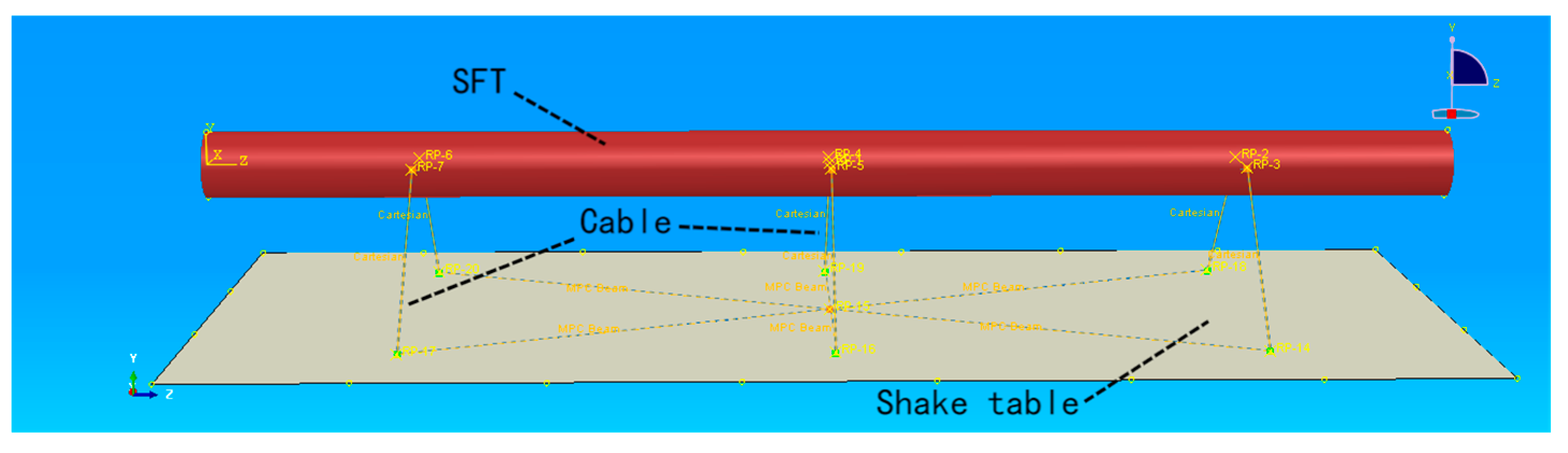
The entire SFT model had a length of 3 m, an outer diameter of 0.16 m, a wall thickness of 4 mm, and a modulus of elasticity of 8.7537 GPa. The model included a 1.5 mm-diameter anchor cable, which contained steel strands spaced 100 cm apart and had a modulus of elasticity of 210 GPa. The anchor cable had a tilt angle of 45°, and the model was placed at a water depth of 80 cm, with a tunnel placement depth of 35 cm. A schematic of the model test is presented in Figure 5.
The seismic excitation waveform applied to the model was a horizontal sine wave with a frequency of 4 Hz, an acceleration amplitude of 0.01× g, and a vibration time of 1 s, as depicted in Figure 7d. Table 3 shows the relationship between the magnitudes of the main physical parameters involved in the actual tests and the similarity constants, i.e., the ratios of the model physical indicators to the prototype’s physical indicators.
3.2. Numerical Modelling
Using the CEL method, a numerical simulation analysis was conducted based on the aforementioned model test. The SFT tube body was set as a rigid body and was simulated using Lagrangian solid elements. The water body was simulated using Eulerian elements, with a density of 1000 kg/m3, a viscosity of 0.001 Pa·s, and a speed of sound of 1480 m/s. The ground containing the shaking table was simulated using rigid shell elements, and the anchor cable system was simulated using simplified spring elements. The anchor cable and the shaking table surface were hinged, as was the submerged floating tunnel section. To simulate the relaxation of the anchor cable, bilinear stiffness was introduced.
The anchor cable tensile stiffness, denoted as Ln, is a constant which is determined using the anchor cable modulus of elasticity (E) and its cross-sectional area (A). When the instantaneous length (Li) of the anchor cable was greater than the unstretched length (original length), Ln remained constant. However, when the transient length was less than the original length, the anchor cable relaxed, and Ln became zero.
The contact between the SFT tube and the fluid was defined as a smooth hard contact, which meant that no mutual intrusion was allowed in the normal direction. The tangential friction coefficient was set to 0.1. A fluid-free surface boundary was used on the surface of the water body, and the fluid velocity on all four sides of the water body was set to zero, ensuring that the fluid flowed only within the grid. An energy dissipation treatment was applied around the water body, and a fixed boundary was applied at the bottom of the water tank. The model dimensions and other physical parameters were the same as those reported by Sun and Chen [17,18]. The model comprised 158,006 elements and 169,020 nodes, and is shown in Figure 6.
3.3. Results Analysis
The numerical simulation was conducted in two steps, the first being a static equilibrium calculation, and the second being a dynamic seismic response calculation. In the latter, a sinusoidal seismic wave was applied horizontally to the bottom of the model, and a seismic time course analysis was conducted. Figure 7 shows comparisons of the time curve of the horizontal acceleration at the center of the SFT body, the horizontal hydrodynamic load–time curve on the outer surface of the tube body, and the time curve of the axial force of the anchor cable, with the experimental results reported by Sun and Chen [17,18]. The hydrodynamic load on the outer surface of the tube body mainly comprised frictional resistance and differential pressure resistance. The former represented the frictional force generated by the water body tangentially on the surface of the tube body and was a direct manifestation of the viscosity of the water body. The latter was an indirect manifestation of the viscosity of the water body, and it was largely caused by the reciprocal vibration of the tube body in the horizontal direction, which led to the water body alternately horizontally separating to the left and right of the surface of the tube body, thus producing pressure differences in the horizontal direction. The calculation results showed that the hydrodynamic load in the vertical direction at this time was much smaller than that in the horizontal direction, and was therefore not chosen as the hydrodynamic load in the vertical direction.
4. SFT Dynamic Frequency Response Analysis
To investigate the frequency response characteristics of the submerged floating tunnel in water, a series of sinusoidal seismic waves, with frequencies ranging from 1 Hz to 15 Hz and an amplitude of 0.01× g, was applied to the bottom of the aforementioned numerical model. The dynamic response of the SFT model under each seismic wave frequency was analyzed, and the peak values of each response indicator were recorded and statistically analyzed. The results are presented in Figure 8.
It is evident from the figure that, when the seismic wave frequency was 11 Hz, the horizontal hydrodynamic load, horizontal acceleration, and cable force of the tube body reached their maximum values (51.7 Pa, 0.777 m/s2, and 36 N, respectively). This indicates that the horizontal self-oscillation frequency of the SFT model was approximately 11 Hz. According to the corresponding similarity constant, this implies that the horizontal self-oscillation frequency of the prototype of the tunnel model was approximately 1.5 Hz.
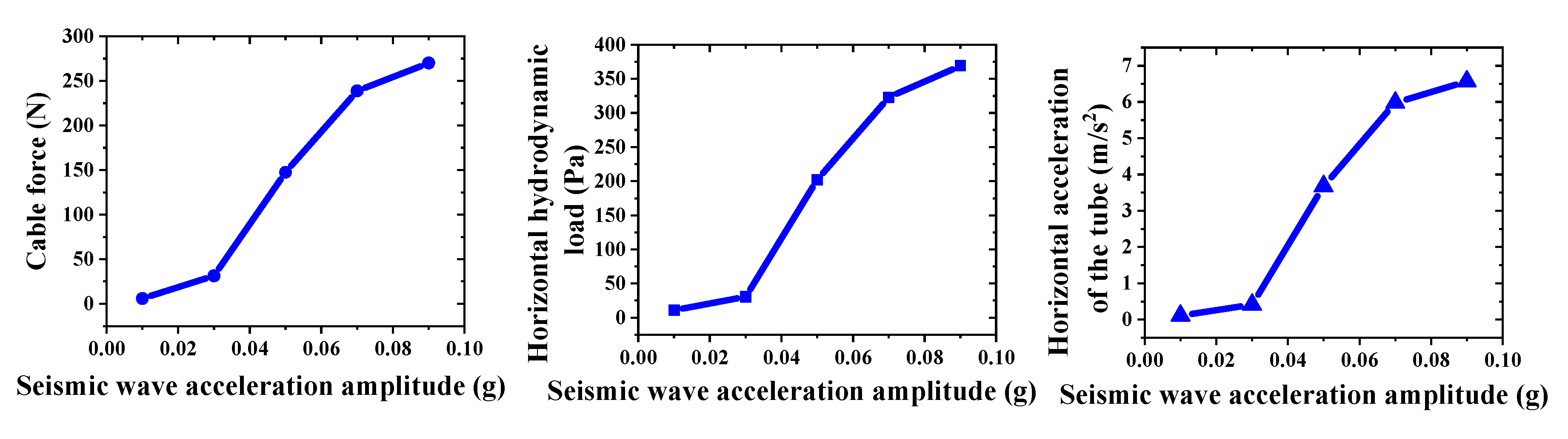
Next, the seismic response of the SFT under the same horizontal sinusoidal seismic wave, with a frequency of 4 Hz and a vibration time of 1 s, was investigated. The acceleration amplitude was adjusted to 0.03× g, 0.05× g, 0.07× g, and 0.09× g, and the peak horizontal hydrodynamic load, horizontal acceleration, and cable force were recorded and analyzed. The results are presented in Figure 9. We provide the tension time history curves of the cable under various conditions in Supplementary Materials Figures S8 and S9, further illustrating the dynamic changes in the tension.
It can be observed that the dynamic response indices of the SFT exhibited a gradual increase when the seismic acceleration amplitude ranged from 0.01× g to 0.03× g. However, a noticeable inflection point and a sharp increase in the dynamic response indices occurred when the seismic acceleration amplitude was between 0.05× g and 0.08× g. When the seismic acceleration amplitude reached between 0.08× g and 0.09× g, the dynamic response indices of the SFT continued to increase, but did so more slowly than before. Based on the similarity constants between the simulation and the model test provided in Table 3, the following dynamic response indices of the prototype SFT were obtained.
where σm is the tensile stress of the model anchor cable, σp is the tensile stress of the prototype anchor cable, Fm is the model cable force, Am is the cross-sectional area of the model cable, Pp is the seismic horizontal water pressure load of the prototype, Pm is the seismic horizontal water pressure load of the model, ap is the acceleration of the prototype tunnel tube body, am is the acceleration of the model tunnel tube body, and N is the prototype/model similarity ratio.
σm = Fm/Am
σp = Nσm
Pp = NPm
ap = am
Table 4 summarizes the tensile stress of the anchor cable in the prototype SFT under the influence of seismic waves of varying intensities, the horizontal ground-vibration water pressure load on the tube body, and the horizontal acceleration of the tube body, as calculated using Equations (7)–(10).
As shown in Table 4, the maximum tensile stress of the anchor cable in the prototype SFT was 535.03 MPa when the seismic wave acceleration strength was 0.03× g, which is within the ultimate tensile strength of the steel strand (1960 MPa; Li et al., 2022 [3]). However, the tensile stress of the anchor cable in the prototype SFT was 4175 MPa when the seismic wave acceleration strength was 0.05× g, which far exceeds the ultimate tensile strength of the steel strand. Therefore, the calculation shows that the cable tension component of this SFT was the most affected parameter under seismic action. Thus, in real-life applications of this SFT, the tensile strength of the cable would need to be appropriately increased to ensure that the cable had a sufficient level of safety redundancy. Additionally, based on the tensile strength performance of the steel strands during seismic activity, it was found that the seismic warning threshold for the SFT was 0.03× g. Therefore, in real-life applications of this SFT, an earthquake early warning alarm would be needed when the motion acceleration reached this level, allowing the operating company to have ample time to implement earthquake response measures.
The horizontal acceleration of the tube body significantly increased as the seismic wave strength increased, and the peak acceleration of the prototype SFT tube body was much larger than the peak acceleration of the corresponding seismic wave, resulting in an amplification effect. This might have been due to the interaction between the tube body and the anchor cable vibration under seismic action, causing an increase in the acceleration response of the tube body. Additionally, the interaction between a seabed-anchored cable and the seabed itself under the action of seismic waves would further increase the acceleration response of the tube body of an SFT. Therefore, the seismic design of an SFT should include measures to suppress this interaction, such as dampers applied to the anchor cables.
5. Conclusions
Few scholars have employed the CEL method to numerically simulate the dynamic response of SFTs. In this study, two simulated examples were explored to demonstrate the reliability of the CEL method for calculating both one-way and two-way fluid–structure coupling problems. Based on this, a CEL numerical model of an SFT was established, and its results agree well with those of previously published shaking table experiments, indicating that the CEL method can effectively simulate the dynamic response of SFTs under seismic effects. Finally, the dynamic response of an SFT under an earthquake was analyzed, and the following conclusions were drawn.
- (1)
- The verification of the CEL method in two hypothetical cylindrical flow calculations and a comparison of the results with those of experimental model SFT tests demonstrated that the CEL method is capable of effectively simulating the seismic dynamic response of SFTs.
- (2)
- The natural frequency of an SFT prototype in a water environment was found to be 1.5 Hz. Thus, when conducting the seismic design of the SFT, the response of the structure under earthquake action should be evaluated. In the analysis, it is necessary to consider the matching relationship between the natural frequency of the structure and the frequency of the earthquake wave motion in order to determine the resonance condition of the structure and its corresponding seismic response characteristics.
- (3)
- The seismic warning threshold for the prototype SFT was 0.03× g. Thus, if an SFT based on this prototype is applied in a real-life setting, an earthquake early warning alarm would need to be issued once the ground motion acceleration reached this level. This would ensure that the anchor cable had a sufficient level of safety redundancy, and it would allow the operating company ample time to implement earthquake response measures.
- (4)
- Under seismic conditions, the peak acceleration of the prototype SFT tube body significantly increased, leading to amplification effects. Therefore, in the seismic design of SFTs, the interaction between the tube body, anchor cable, and seabed should be the foremost consideration.
Overall, our findings reveal that the CEL method’s potential applications in fluid–structure interaction analysis transcend traditional boundaries, demonstrating its remarkable adaptability in simulating the responses of intricate underwater structures under seismic conditions. This discovery not only expands the realm of CEL method applications, but also introduces a novel and promising numerical simulation approach for seismic research on submerged floating tunnels. However, it is worth emphasizing that our research results are preliminary and require further investigation and improvements. While the successful application of the CEL method in simulating seismic responses of submerged floating tunnels provides robust initial support for its reliability and effectiveness in engineering applications, further refinement and validation are crucial to ensure its widespread adoption and optimal performance.
The seismic analysis of SFTs is complex due to the vibration of their structures being affected not only by hydrostatic pressure, but also by dynamic water pressure. A water body can cause changes in the frequency, vibration pattern, and damping of SFT structures, resulting in coupling between structural vibration and the water body’s seismic response. Additionally, the seismic effect of submarine soil deformation would directly affect the anchorage foundation of an SFT and its tunnel section. This research provides a strong technological foundation and data support for further studies of the dynamic interaction mechanisms between a water body, an SFT, its anchored foundations, and soil bodies under seismic conditions.
Supplementary Materials
The following supporting information can be downloaded at: https://www.mdpi.com/article/10.3390/app14093589/s1, Figure S1: Schematic Diagram of the Experimental [16,18]; Figure S2: Schematic Diagram of Numerical Models; Figure S3: Schematic Diagram of the Experimental and Numerical Models; Figure S4: Velocity field cloud images at different stages of bidirectional fluid-structure coupling of the model; Figure S5: Comparison of numerical and empirical drag force solutions; Figure S6: The schematic diagram of operator splitting for the Euler equations; Figure S7: The Volume of Fluid method involves the representation of material volume fraction and the schematic diagram of material boundaries; Figure S8: Variation curve of cable tension under the action of sinusoidal waves with different peak accelerations; Figure S9: Variation curve of cable tension under the action of sinusoidal waves with different frequencies; Table S1: Comparison of the empirical and simulated drag force calculation results (where V represents the horizontal velocity of the column).
Author Contributions
Conceptualization, X.C.; methodology, H.L.; software, H.L.; validation, X.C., H.L. and H.P.; formal analysis, H.L.; investigation, H.L.; resources, H.L.; data curation, H.L.; writing—original draft preparation, H.L.; writing—review and editing, X.C.; visualization, H.L.; supervision, X.C.; project administration, H.L.; funding acquisition, X.C., H.L. and H.P. All authors have read and agreed to the published version of the manuscript.
Funding
This research was funded by the Basic Research Business Special Fund of Central Public Welfare Research Institutes, with the project number DQJB23K41.
Institutional Review Board Statement
Not applicable.
Informed Consent Statement
Not applicable.
Data Availability Statement
The data that support the findings of this study are available from the corresponding author, upon reasonable request.
Conflicts of Interest
The authors declare no conflict of interest.
References
- China Association for Science and Technology publishes 60 major scientific problems and engineering and technical problems in 12 fields. J. China Railw. Soc. 2018, 40, 24, 53, 87, 135.
- Wu, Z.; Wang, D.; Ke, W. Experimental investigation for the dynamic behavior of submerged floating tunnel subjected to the combined action of earthquake, wave, and current. Ocean Eng. 2021, 239, 109911. [Google Scholar] [CrossRef]
- Li, H.; Cheng, X.; Yu, H.; Fu, D. Seismic response simulation of submerged floating tunnel with tension legs: A case study on the Qiongzhou Strait Crossing Tunnel Project. Mod. Tunnel. Technol. 2022, 59, 146–154. [Google Scholar]
- Xiang, Y.; Yang, Y.; Bai, B. Methods for Analyzing Seismic Response of Submerged Floating Tunnel and Research Development. In Proceedings of the 14th International Conference on Vibration Problems, Crete, Greece, 1–4 September 2019; Springer Nature: Singapore, 2019. [Google Scholar]
- Wu, Z.; Ni, P.; Mei, G. Vibration response of cable for submerged floating tunnel under simultaneous hydrodynamic force and earthquake excitations. Adv. Struct. Eng. 2018, 21, 1761–1773. [Google Scholar] [CrossRef]
- Fogazzi, P.; Perotti, F. The dynamic response of seabed anchored floating tunnels under seismic excitation. Earthq. Eng. Struct. Dyn. 2000, 29, 273–295. [Google Scholar] [CrossRef]
- Martinelli, L.; Barbella, G.; Feriani, A. Modeling of Qiandao Lake submerged floating tunnel subject to multi-support seismic input. Procedia Eng. 2010, 4, 311–318. [Google Scholar] [CrossRef]
- Martinelli, L.; Barbella, G.; Feriani, A. A numerical procedure for simulating the muti-support seismic response of SFT anchored by cables. Eng. Struct. 2011, 33, 2850–2860. [Google Scholar] [CrossRef]
- Brancaleoni, F.; Castellani, A.; D’Asdia, P. The response of submerged tunnels to their environment. Eng. Struct. 1989, 11, 47–56. [Google Scholar] [CrossRef]
- Martire, G.; Faggianoa, B.; Mazzolani, F.M.; Zollo, A.; Stabile, T. Seismic analysis of an SFT solution for the Messina Strait crossing. Procedia Eng. 2010, 4, 303–310. [Google Scholar] [CrossRef]
- Xiao, J.; Huang, G. Transverse earthquake response and design analysis of SFT with various shore connections. Procedia Eng. 2010, 4, 233–242. [Google Scholar] [CrossRef]
- Chen, W.; Huang, G. Seismic wave passage effect on the dynamic response of SFT. Procedia Eng. 2010, 4, 217–224. [Google Scholar] [CrossRef]
- Chao, C.F.; Xiang, Y.Q.; Lin, J.P. Patterns of cable VIV suppression based on the fluid-structure interaction. Mech. Eng. 2015, 37, 725–730. (In Chinese) [Google Scholar]
- Chao, C.F.; Xiang, Y.Q.; Yang, C. Experiments on dynamic fluid-structure coupled responses of anchor cables of submerged floating tunnel. J. Vib. Shock 2016, 3, 158–163. (In Chinese) [Google Scholar]
- Sun, S.; Chen, J. Study on hydrodynamic pressure of SFT under earthquake-SV wave. J. Disast. Prev. Mitig. Eng. 2006, 4, 425–430. (In Chinese) [Google Scholar]
- Sun, S.; Chen, J. Study on dynamic water pressure of undersea anchorage SFT-P wave. J. Harbin Inst. Technol. 2008, 8, 1292–1296. (In Chinese) [Google Scholar]
- Chen, J.; Li, J.; Sun, S. Experimental and numerical analysis of submerged floating tunnel. J. Cent. South Univ. 2012, 19, 2949–2957. [Google Scholar] [CrossRef]
- Sun, S.; Chen, J. Dynamic Response Analysis of SFT. Ph.D. Thesis, Dalian University of Technology, Dalian, China, 2008. (In Chinese). [Google Scholar]
- Zhang, H.; Yang, Z. A global review for the hydrodynamic response investigation method of submerged foating tunnels. Ocean Eng. 2021, 225, 108825. [Google Scholar] [CrossRef]
- Zhu, Y. Wave Mechanics in Ocean Engineering; Tianjin University Press: Tianjin, China, 1991. [Google Scholar]
- Matsui, T.; San, K.C. Finite element slope stability analysis by shear strength reduction technique. Soils Found. 1992, 32, 59–70. [Google Scholar] [CrossRef]
- Shiau, J.S.; Lyamin, A.V.; Sloan, S.W. Bearing capacity of a sand layer on clay by finite element limit analysis. Can. Geotech. J. 2003, 40, 900–915. [Google Scholar] [CrossRef]
- Hirt, C.W.; Nichols, B.D. Volume of fluid (VOF) method for the dynamics of free boundaries. J. Comput. Phys. 1981, 39, 201–225. [Google Scholar] [CrossRef]
- Noh, W.F. CEL: A Time-Dependent Two Space-Dimensional, Coupled Eulerian-Lagrangian Code; Lawrence Radiation Laboratory: Livermore, CA, USA, 1964. [Google Scholar]
- Hajivalie, F.; Yeganeh-Bakhtiary, A.; Houshanghi, H.; Gotoh, H. Euler–Lagrange model for scour in front of vertical breakwater. Appl. Ocean Res. 2012, 34, 96–106. [Google Scholar] [CrossRef]
- Mittal, V.; Chakraborty, T.; Matsagar, V. Dynamic analysis of liquid storage tank under blast using coupled Euler–Lagrange formulation. Thin-Walled Struct. 2014, 84, 91–111. [Google Scholar] [CrossRef]
- Cheng, Z.; Chauchat, J.; Hsu, T.J.; Calantoni, J. Eddy interaction model for turbulent suspension in Reynolds-averaged Euler–Lagrange simulations of steady sheet flow. Adv. Water Resour. 2017, 111, 435–451. [Google Scholar] [CrossRef]
- ABAQUS, Version 2016. EF Documentation. Dassault Systèmes: Vélizy-Villacoublay, France, 2016.
- Roshko, A. On the Development of Turbulent Wakes from Vortex Streets; NASA: Washington, DC, USA, 1953. [Google Scholar]
- Taneda, S. Downstream development of the wakes behind cylinders. J. Phys. Soc. Jpn. 1959, 14, 843–848. [Google Scholar] [CrossRef]
- Sarpkaya, T. Vortex-induced oscillations: A selective review. J. Appl. Mech. 1979, 46, 241–258. [Google Scholar] [CrossRef]
- Xiao, S. Research on Constitutive Model and Numerical Simulation of Sand Rheology under Low Effective Stress; Tsinghua University: Beijing, China, 2020. (In Chinese) [Google Scholar]
Figure 1.
Simplified modeling diagram of cylindrical flow.

Figure 2.
Velocity clouds and vector diagrams of simulated circular cylinder flow at various Reynolds numbers (Re) (the left and right figures correspond to the same time).
Figure 2.
Velocity clouds and vector diagrams of simulated circular cylinder flow at various Reynolds numbers (Re) (the left and right figures correspond to the same time).


Figure 3.
Velocity field clouds at different stages in a model of two-way fluid–solid coupling.

Figure 4.
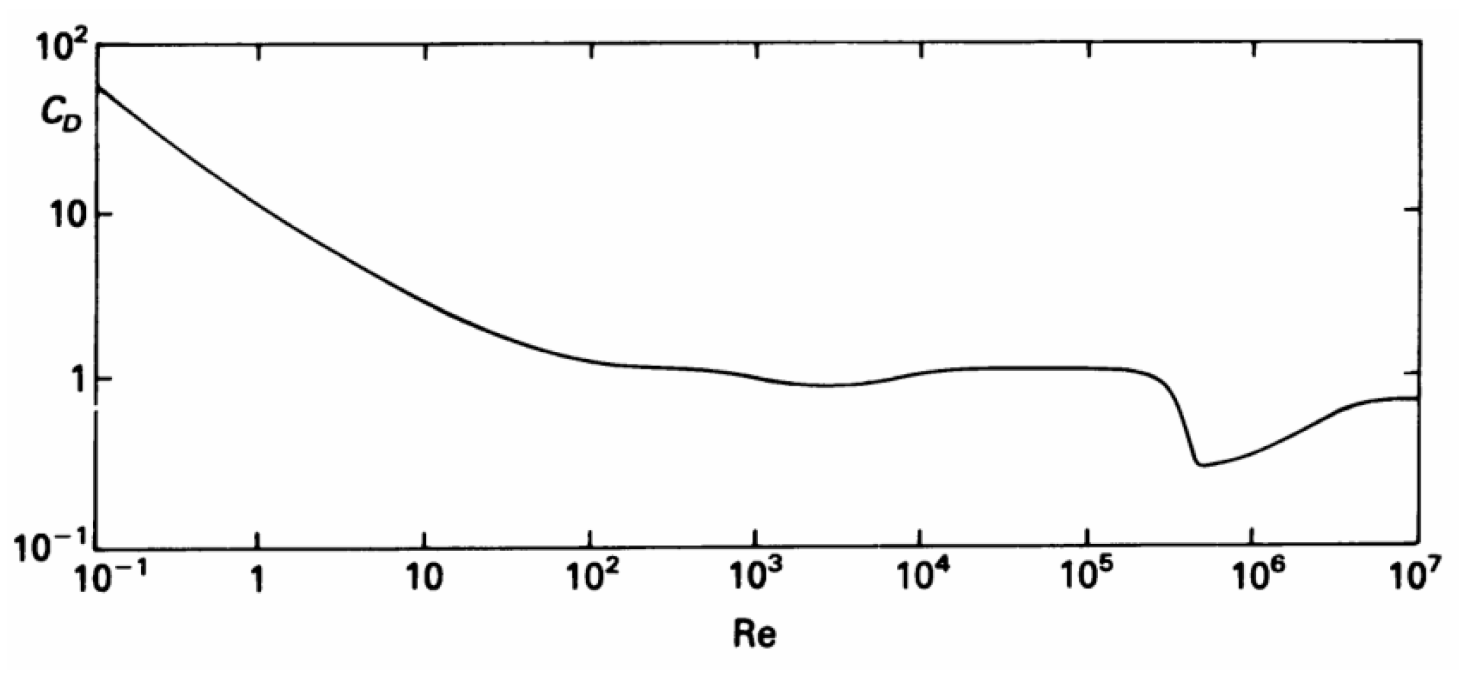
Empirical curve of the drag force coefficient of circular cylinder flow vs. Reynolds number (Re) [20].
Figure 4.
Empirical curve of the drag force coefficient of circular cylinder flow vs. Reynolds number (Re) [20].

Figure 5.
Experimental diagram of the submerged floating tunnel (SFT) model.

Figure 6.
Numerical model diagram of SFTs. (a) Numerical model diagram of a submerged floating tunnel (SFT) simulated using the coupled Eulerian–Lagrangian method. (b) SFT model (numbers are anchor cable numbers).
Figure 6.
Numerical model diagram of SFTs. (a) Numerical model diagram of a submerged floating tunnel (SFT) simulated using the coupled Eulerian–Lagrangian method. (b) SFT model (numbers are anchor cable numbers).

Figure 7.
Comparison of numerical and experiment solutions.

Figure 8.
Peak value of each dynamic response index at different frequencies.

Figure 9.
Peak value of each dynamic response index under different seismic wave intensities.


Table 1.
Relationship between vortex shedding and Reynolds number (Re) [31].
Table 1.
Relationship between vortex shedding and Reynolds number (Re) [31].
 | 15 < Re < 40: A group of small, fixed vortices appeared after a cylinder |
 | 150 < Re < 300,000 Periodic alternating turbulent vortex discharge occurred |
Table 2.
Comparison of empirically calculated and simulated values of drag force at various Reynolds numbers (Re).
Table 2.
Comparison of empirically calculated and simulated values of drag force at various Reynolds numbers (Re).
| V (m/s) | CD | Re | Drag Force: Empirical Value (N) | Drag Force: Simulated Value (N) | Relative Error % |
|---|---|---|---|---|---|
| 0.5 | 1.08 | 10,000 | 2.7 | 2.9 | 7.4 |
| 1 | 1.12 | 20,000 | 11.2 | 10.5 | 6.3 |
| 2 | 1.13 | 40,000 | 45.2 | 44.4 | 1.77 |
| 5 | 1.1 | 100,000 | 275 | 256.2 | 6.8 |
Relative error = ABS (|simulated solution − empirical solution|/empirical solution), CD is the drag force coefficient and was taken from Figure 4, and V is the horizontal velocity of the column.
Table 3.
Model test similarity constants.
| Physical Indicators | Dimensional System [L][ρ][ε][g] | Similarity Constant (N = 50) | |
|---|---|---|---|
| Geometric features | Geometric dimension | [L] | 1/N |
| Area | [L]2 | 1/N2 | |
| Inertia moment | [L]4 | 1/N4 | |
| Material behavior | Density | [ρ] | 1 |
| Elasticity modulus | [L][ρ][g][ε]−1 | 1 | |
| Mass | [ρ][L]3 | 1/N3 | |
| Dynamic characteristics | Input vibration acceleration | [g] | 1 |
| Field acceleration | [g] | 1 | |
| Force | [ρ][L]3[g] | 1/N3 | |
| Input vibration time | [L]0.5[ε]0.5[g]−0.5 | 1/N0.5 | |
| Vibrational frequency | [L]−0.5[ε]−0.5[g]0.5 | N0.5 | |
| Dynamic response acceleration | [g] | 1 | |
| Dynamic response stress | [ρ][L][g] | 1/N | |
| Dynamic response strain | [ε] | 1 |
Table 4.
Peak values of the dynamic response indices of the prototype and model under various seismic wave intensities.
Table 4.
Peak values of the dynamic response indices of the prototype and model under various seismic wave intensities.
| Seismic Wave Acceleration (× g) | Cable Force (MPa) | Horizontal Hydrodynamic Load (Pa) | Horizontal Acceleration of the Tube (m/s2) | |||
|---|---|---|---|---|---|---|
| σm | σp | Pm | Pp | ap | am | |
| 0.01 | 3.40 | 169.85 | 11 | 550 | 0.11 | 0.11 |
| 0.03 | 10.70 | 535.03 | 30.5 | 1525 | 0.41 | 0.41 |
| 0.05 | 83.51 | 4175.51 | 202 | 10,100 | 3.68 | 3.68 |
| 0.07 | 135.20 | 6760.08 | 322.8 | 16,140 | 5.98 | 5.98 |
| 0.09 | 152.92 | 7646.14 | 369.2 | 18,460 | 6.57 | 6.57 |
Disclaimer/Publisher’s Note: The statements, opinions and data contained in all publications are solely those of the individual author(s) and contributor(s) and not of MDPI and/or the editor(s). MDPI and/or the editor(s) disclaim responsibility for any injury to people or property resulting from any ideas, methods, instructions or products referred to in the content. |
© 2024 by the authors. Licensee MDPI, Basel, Switzerland. This article is an open access article distributed under the terms and conditions of the Creative Commons Attribution (CC BY) license (https://creativecommons.org/licenses/by/4.0/).
Share and Cite
MDPI and ACS Style
Li, H.; Cheng, X.; Pan, H. Numerical Simulation of a Submerged Floating Tunnel: Validation and Analysis. Appl. Sci. 2024, 14, 3589. https://doi.org/10.3390/app14093589
AMA Style
Li H, Cheng X, Pan H. Numerical Simulation of a Submerged Floating Tunnel: Validation and Analysis. Applied Sciences. 2024; 14(9):3589. https://doi.org/10.3390/app14093589
Chicago/Turabian StyleLi, Hao, Xiaohui Cheng, and Hua Pan. 2024. "Numerical Simulation of a Submerged Floating Tunnel: Validation and Analysis" Applied Sciences 14, no. 9: 3589. https://doi.org/10.3390/app14093589
Note that from the first issue of 2016, this journal uses article numbers instead of page numbers. See further details here.