Effect of Data Augmentation Using Deep Learning on Predictive Models for Geopolymer Compressive Strength

Abstract

In recent years, machine learning models have become a potential approach in accurately predicting the concrete compressive strength, which is essential for the real-world application of geopolymer concrete. However, the precursor system of geopolymer concrete is known to be more heterogeneous compared to Ordinary Portland Cement (OPC) concrete, adversely affecting the data generated and the performance of the models. To its advantage, data enrichment through deep learning can effectively enhance the performance of prediction models. Therefore, this study investigates the capability of tabular generative adversarial networks (TGANs) to generate data on mixtures and compressive strength of geopolymer concrete. It assesses the impact of using synthetic data with various models, including tree-based, support vector machines, and neural networks. For this purpose, 930 instances with 11 variables were collected from the open literature. In particular, 10 variables including content of fly ash, slag, sodium silicate, sodium hydroxide, superplasticizer, fine aggregate, coarse aggregate, added water, curing temperature, and specimen age are considered as inputs, while compressive strength is the output of the models. A TGAN was employed to generate an additional 1000 data points based on the original dataset for training new predictive models. These models were evaluated on real data test sets and compared with models trained on the original data. The results indicate that the developed models significantly improve performance, particularly neural networks, followed by tree-based models and support vector machines. Moreover, data characteristics greatly influence model performance, both before and after data augmentation.

1. Introduction

Concrete stands as the most extensively utilized man-made material worldwide [1]. The incessantly rising demand for concrete translates into a parallel surge in the need for cement, evidenced by a reported 12% increase in 2019 and an anticipated doubling by 2050 [2]. Nonetheless, the production of cement imposes diverse environmental repercussions [2]. Each ton of cement manufactured emits 0.6–1 ton of CO₂, contingent upon production methods, contributing 5–7% to global CO₂ emissions [1]. Additionally, limestone exploitation for cement production triggers water and land pollution, disturbing local ecosystems and biodiversity [3]. Therefore, numerous studies have been conducted to explore alternative materials to replace cement. In recent years, alkali-activated materials, such as geopolymers, have emerged as a promising alternative to OPC-based materials due to their lower carbon footprint and utilization of industrial by-products [4]. Geopolymers are polymeric aluminosilicate cementitious materials that involve industrial wastes (i.e., fly ash, slag, and silica fume) as the precursors under the action of alkaline chemicals such as sodium hydroxide and sodium silicate [5].

Similar to OPC concrete, the strength of geopolymer concrete is influenced by various parameters, including both external and internal factors. External factors such as temperature, duration, curing types, humidity, and air containment play significant roles in determining the strength of geopolymer concrete [6]. On the other hand, internal factors, such as material quality and mixture compositions, also have a substantial impact. Because of the intricate relationships and inconsistencies in precursors and alkaline activators, a mixture proportion can yield a wide range of compressive strengths [7]. Therefore, calculating the distribution and predicting the intensity using empirical and theoretical methods pose significant challenges.

With the growth in ML applications, researchers are increasingly turning to ML to address the problem of compressive strength prediction for geopolymer concrete [8]. ML models heavily rely on large, high-quality datasets and models trained on datasets containing fewer than 1000 data points are prone to overfitting problems [9]. However, according to the research of Li et al. (2022) [9], only 11% of the studies on applying ML to concrete science utilize datasets containing more than 1000 samples. Also, the average sample size is estimated to be 174 [9]. To mitigate the challenge of data scarcity in concrete science, several studies have adopted generative models such as Generative Adversarial Networks (GANs) [10], Conditional Generative Adversarial Networks (CGANs) [11], Cycle-Consistent Deep Generative Adversarial Networks (CDGANs) [11], and TGANs [12,13] to generate synthetic data for ML models. The use of synthetic data has shown significant improvements in model performance, particularly noticeable with TGAN and CDGAN models [11,13]. However, existing research predominantly focuses on generating data for OPC concrete with less emphasis on geopolymer concrete. Meanwhile, geopolymer mixtures involve a more intricate ingredient system including alumino-silicate precursors and alkali activators, which are more complex than the cement–water system of OPC concrete [5]. Moreover, geopolymer precursors exhibit significant variations in chemical composition and reactivity across different factories, regions, and time periods [5]. Conversely, cement exhibits greater standardization in these aspects, resulting in more consistent data collection and synthesis. Consequently, the impact on generating and utilizing synthetic data on geopolymer strength prediction models may differ from that of OPC concrete. However, research focusing on the effectiveness of data augmentation specifically for geopolymer concrete remains limited.

Therefore, this study aims to investigate the ability of TGANs to generate data for geopolymers and the impacts of synthetic data on various algorithms with different mathematical principles and assumptions, including tree-based models, SVM, and neural networks. To achieve this objective, this study uses datasets collected from the open literature to ensure diversity in sources and the chemical composite of precursors. The dataset collected for this study consists of 930 instances. Specifically, 10 variables are considered as inputs, including the content of fly ash (FA), slag (S), sodium silicate (SS), sodium hydroxide (SH), superplasticizer (SP), fine aggregate (Fag), coarse aggregate (Cag), added water (W), curing temperature (CT), and specimen age (Age). The output of the models is the compressive strength (CS). Subsequently, a TGAN was employed to generate data pertaining to fly ash- and slag-based geopolymer concrete mixtures and their corresponding strengths based on the collected dataset. The generated data was then utilized to train different models, including LightGBM, SVM, and cascade forward neural networks (CFNNs). Next, models using synthetic data will be compared with models using original data with evaluation metrics such as R-squared (R²), Mean Absolute Error (MAE), Root Mean Squared Error (RMSE), Mean Absolute Percentage Error (MAPE), Root Mean Square Residual (RSR), and Weighted Mean Absolute Percentage Error (WMAPE). Additionally, SHAP analysis was performed to facilitate the interpretation of model performance and data influence.

2. Literature Review

2.1. Machine Learning Models for Prediction

In recent years, there has been an increasing number of studies using ML to predict the strength of geopolymers. Among these, artificial neural networks (ANNs) have emerged as the most prominent, with numerous studies demonstrating promising prediction capabilities [14,15,16]. Alongside ANNs, convolutional neural networks (CNNs) [17] and deep neural networks (DNNs) [18] are also utilized. Additionally, tree-based algorithms including decision tree (DT) [19], random forest (RF) [20], LightGBM [20], and MP5-tree [21] are employed, showing advantages in model interpretation and handling skewed data. Similarly, recently emerged algorithms known as gene expression programming (GEP) [22] and its variants exhibit superior model interpretation capabilities compared to neural network models. SVM [15] is another popular algorithm that yields results comparable to ANN. To further enhance model performance, various optimization algorithms such as grey wolf optimizer (GWO) [23] and particle swarm optimization (PSO) [23] are employed. Additionally, stacked and ensemble models are utilized in several studies, demonstrating improved performance compared to individual models.

The input variables in these studies typically include mixture proportions, chemical compositions of precursors, specimen age, and external factors such as curing temperature and curing regimes.

Table 1. Statistical description for the features in the dataset.

Refs.	ML Technology	Dataset	Inputs
[24]	LR, EL, SVMR, GPR, optimized EL, optimized SVMR, optimized GPR	275	Fly ash, coarse aggregate, fine aggregate, Na2SiO3, NaOH, SiO2, molarity of NaOH and Na2O
[19]	DT, AdaBoost, RF	363	Water/solids ratio, molarity of NaOH, gravel 4/10 mm, gravel 10/20 mm, Na2SiO3, NaOH, fly ash, GGBS, fag
[20]	RF, GB, AdaBoost, DT, lightGBM, XGB, kNN, MVR, GPR, CatB	158	Fly ash, superplasticizer, extra water added, Na2SiO3, NaOH, coarse aggregate, fine aggregate, slag, specimen age, rest period, curing temperature, molarity, alkali/binder, and Na2SiO3/NaOH
[14]	ANN, MLR, MNLR	289	Fly ash, slag, rest period, curing temperature, age, NaOH/Na2SiO3, superplasticizer, extra water, molarity of NaOH, alkali/binder, coarse aggregate, fine aggregate
[15]	SVM, DT, RFR	75	Molarity of NaOH, curing temperature, age, % of Na2SiO3, NaOH, fly ash, coarse aggregate, fine aggregate, Na2SiO3, NaOH
[25]	ANN, M5P, LR, MLR	220	Alkali/binder, fly ash, Si/Al of fly ash, GGBS, Si/Ca of GGBS, coarse aggregate, fine aggregate, Na2SiO3, NaOH, Na2SiO3/NaOH, molarity of NaOH
[26]	ANN, MARS	208	Water/solid ratio, alkali/binder, Na-Silicate/NaOH, fly ash/slag ratio, NaOH molarity
[27]	RF, GBR, AdaBoost	321	GGBS, Na2SiO3 + NaOH (total alkali), coarse aggregate, fine aggregate, water, water/binder, age
[23]	LR, GA, PSO, SVR, GWO, Differential Evolution	268	Water, curing temperature, water/binder, GGBFS/ binder, coarse aggregate, fine aggregate, superplasticizer
[28]	ANN	81	GGBS, silica fume
[16]	ANN, BLR	625	Na2O:SiO2, Na2O:H2O, GGBFS:H2O, molarity of NaOH, Na2SiO3/NaOH, AS/GGBS, GGBS/water
[29]	DT, Bagging, LightGBM	351	Specimen age, molarity of NaOH, natural zeolite, silica fume, GGBFS
[22]	ANFIS, ANNs, GEP	245	Chemical composition of fly ash, mixing procedures, curing regime, activator content, fine aggregate, coarse aggregate, water, activator/fly ash, and molarity of NaOH

LR: Linear Regression, EL: Elastic Net, SVM: Support Vector Machine, GPR: Gaussian Process Regression, DT: Decision Tree, AdaBoost: Adaptive Boosting, RF: Random Forest, GB: Gradient Boosting, lightGBM: Light Gradient Boosting Machine, XGB: XGBoost, kNN: k-Nearest Neighbors, MVR: Multivariate Regression, CatB: CatBoost, ANN: Artificial Neural Network, MLR: Multinomial Logistic Regression, MNLR: Multinomial Naive Bayes Logistic Regression, M5P: M5’ Model Tree, MARS: Multivariate Adaptive Regression Splines, GA: Genetic Algorithm, PSO: Particle Swarm Optimization, GWO: GreyWolf Optimizer, BLR: Bayesian Linear Regression, Bagging: Bootstrap Aggregating, LSBoost: Least Squares Boosting, ANFIS: Adaptive Neuro-Fuzzy Inference System, GEP: Gene Expression Programming.

presents the inputs, dataset sizes, and algorithms used in some related studies.

Table 1 indicates that neural network algorithms, tree-based models, and support vector algorithms are of significant interest. Furthermore, it is observed that the sample size in the majority of studies is insufficient for ML models, particularly when utilizing neural networks and deep learning. This scarcity of data, coupled with data complexity, can lead to high-dimensionality and data-bias problems [30]. Hence, data augmentation becomes essential in scenarios of limited experimental data availability.

2.2. Data Augmentation

In the field of concrete science, GANs are employed as powerful tools for data generation in conjunction with ML models. One notable application is the generation of images. For example, Yasuno et al. (2020) [10] utilized GANs to generate damaged images by mapping tri-categorical labels to real damaged images through image-to-image translation. In another study, Dunphi et al. (2022) [31] investigated the performance of a CNN architecture for multiclass damage detection on concrete surfaces.

Recently, several variants of GANs have been used for generating tabular data for concrete strength prediction problems. The study of Marani et al. (2020) [13] used TGAN to generate 6513 plausible synthetic data for RF, extra trees (ETR), and GBR models from 810 experimental instances. The results indicate that the developed models achieved outstanding predictive performance. GAN, DCGAN, and WGAN were used to generate data in the study by Chen et al., 2022 [11]. DCGAN performed better than the remaining models and helped improve the performance of deep learning models. In another study, TGAN was used in generating synthetic data on the shear capacity of FRP-reinforced concrete beams [13]. The study demonstrates that the TGAN technique could address the lack of availability of experimental datasets in engineering problems by synthesizing numerous probable data points.

The previous studies evidence that TGANs are a powerful tool for generating tabular data, particularly in the case of concrete gradation and strength. In light of this, the present study employs a TGAN for data generation to examine the effects of the synthetic data on the performance of various models.

3. Methodology

3.1. Tabular Generative Adversarial Networks

To address the scarcity of available data, GANs have been proposed as a solution for generating synthetic data from original data [32]. GANs draw inspiration from the concept of zero-sum games in game theory. In this framework, there exist two networks: a generator network (G) and a discriminator network (D). The GAN leverages the independent and adversarial relationship between G and D to train and produce specified data samples. G receives a random noise vector as input, from which it generates new relevant data. D, on the other hand, receives both the actual data and the data generated by G as input. These two networks engage in continuous competition, each pursuing its own objectives independently. As the distribution of the generated data gradually converges to that of the real data, it becomes increasingly challenging for D to differentiate between them, signaling the completion of the GAN model training. Remarkably, various GAN variations have emerged for generating synthetic data, spanning images, text, and numerical data, among others. One notable advancement is the TGAN, which excels in generating both discrete and continuous tabular data simultaneously, showcasing promising efficiency [12].

TGANs employ the Adam optimizer for training, with a long short-term memory (LSTM) network acting as the generator and a multi-layer perceptron (MLP) functioning as the discriminator. One interesting feature of a TGAN is its capability to transform non-Gaussian distributions into continuous columns using a clever mode-specific normalization method. This enables it to capture the inherent distribution of the original data and effectively model the relationships between features. In the optimization phase, the loss function incorporates both KL divergence and cluster vector terms to enhance model stability. The formulation of the loss function is provided in Equations (1) and (2).

Generator:

$$Los{s}_G=-E_{zN(0,1)}logD\left(G\left(z\right)\right)+\sum _{i=1}^{n_c}KL(u_i^{\prime },u_i)+\sum _{i=1}^{n_c}KL(d_i^{\prime },d_i)$$

(1)

Discriminator:

$$Los{s}_D=-E_{v_{1:n_c},u_{1:n_c},d_{1:n_d}P\left(T\right)}logD\left(v_{1:n_c,u1:n_c,d1:n_d}\right)+E_{zN(0,1)}logD\left(G\left(z\right)\right)$$

(2)

where $u_i^{\prime }$ and $d_i^{\prime }$ are synthetic data, $u_i$ and $d_i$ are original data, and $n_c$ and $n_d$ are the numbers of continuous and discrete variables, respectively.

Figure 1 illustrates the architecture of a TGAN. In this investigation, a TGAN was trained utilizing the TGAN package implemented in Python.

3.2. Machine Learning Predictive Models

Based on a preliminary literature review, this study recognizes tree-based algorithms, support vector algorithms, and neural networks as prominent choices for intensity prediction tasks in geopolymers. Consequently, the study intends to evaluate how the utilization of synthetic data impacts the performance of these models. Specifically, LightGBM, SVM, and CFNN were investigated to represent the aforementioned three algorithm groups. The advantages and disadvantages of these algorithms in compressive strength prediction scenarios are summarized in

Table 2. Comparison of the three models.

Algorithms	Advantages	Disadvantages
LightGBM [33]	- Efficient and faster training compared to traditional gradient boosting algorithms - Handles large-scale data and high-dimensional features effectively - Automatically handles missing values - Resistant to overfitting and provides good accuracy and generalization performance	- Limited support for certain data types, such as text or images (requires feature engineering) - Can be sensitive to noise or outliers in the data - Model complexity can increase with the number of trees
SVM [34]	- Effective for high-dimensional data and can handle large feature spaces - Provides good generalization performance, even with limited training data - Robust to overfitting and works well with non-linear data by using kernel tricks	- Training time can be slow for large datasets - Not well-suited for large datasets with noise or outliers - Limited interpretability compared to some other models
CFNN [35,36]	- Highly versatile and can model complex non-linear relationships - Capable of automatic feature extraction and learning hierarchical representations - Scalable to large datasets with the availability of computational resources	- Require large amounts of training data to achieve good performance - Can be computationally expensive, especially for deep architectures - Limited interpretability and often considered as “black boxes”

. In the context of this study, these ML techniques do not require the data to follow a normal distribution, making them suitable for the collected dataset in this study.

3.3. LightGBM

Light GBM, developed by Microsoft Research [37], is a variant of Gradient Boosting Decision Trees based on a decision-tree technique. LightGBM constructs trees leaf by leaf, employing a histogram-based technique to partition leaf nodes. This approach yields notable efficiency and memory savings [38]. Although the leaf-wise tree growth enhances model complexity, LightGBM can achieve greater accuracy improvements with each iteration of the algorithm. However, this method poses a significant risk of overfitting, which is addressed through regularization terms. To render LightGBM a swift, effective, and dependable ensemble method, two strategies are employed: gradient-based one-side sampling (GOSS) and exclusive feature bundling (EFB) [38]. GOSS selectively retains samples with higher gradients during the training phase, as they contribute more to information gain, discarding those with lower gradients. Consequently, compared to traditional methods like DT, RF, and gradient boosted decision trees (GBDT) that examine all data for information gain calculation, LightGBM with GOSS significantly reduces computation time. On the other hand, EFB clusters exclusive features together in a sparse feature space, reducing dimensionality and enhancing efficiency. Particularly in scenarios involving high feature dimensions, LightGBM combined with EFB substantially enhances model efficiency and scalability compared to standard approaches (e.g., RF, DT, and GBDT). Consequently, this adaptation markedly accelerates the computation process and minimizes memory usage while preserving prediction accuracy.

To enhance the performance of the LightGBM in this study, grid search cross-validation was employed to explore various hyperparameter combinations for LightGBM, resulting in the selection of optimal values: n_estimators = 300, learning_rate = 0.3, max_depth = 10, num_leaves = 30, and min_child_samples = 20.

3.4. Support Vector Machine (SVM)

The SVM method employs non-linear decision boundaries to carry out regression and classification tasks, offering significant flexibility within the feature space where these boundaries reside. It relies on principles of statistical learning and structural risk reduction. However, SVM parameters are not predetermined, and there is no prior knowledge about the distribution of inputs and outputs. During training, input and output values are aligned in training sets, enabling the derivation of decision functions to classify new datasets based on these alignments. The equation representing the SVM-derived plane is expressed as Equation (4) [39].

$$f\left(x\right)=(w,x)+b$$

(3)

In this context, the weight vector w and the scalar constant b play crucial roles. The training data is denoted by n-dimensional vector x. By computing the dot product of w and x, and adding the scalar b, the function’s result is obtained. Each training datum is represented by an n-dimensional vector. The dataset, comprising m data points, assigns each data point to one of the elements in the set $y\in \{+1,-1\}$. The SVM model illustrates class samples as points in space, aiming to separate instances of different classes with an open vector, maximizing the space between them [39].

In this work, SVM hyperparameters were fine-tuned, leading to optimal parameters: C = 133, epsilon = 0.02, and gamma = 0.7.

3.5. Cascade forward Neural Networks (CFNNs)

CFNN is a specialized form of the MLP with a unique network structure. Generally, CFNN includes an input layer, one or more hidden layers, and an output layer, mirroring the architecture of the MLP model. However, unlike the MLP, which employs a feedforward network structure to transmit data from the input to output layers via hidden layers, CFNN introduces additional direct connections between the input and output layers [40]. This difference results in CFNN having a denser interconnection of weights and biases compared to the traditional MLP. The CFNN architecture in this study is depicted in Figure 2.

The CFNN model constructs its cascade architecture within the network by incorporating newly added neurons and their connections. The additional connections between the input layer and subsequent layers potentially enhance the learning rate of the network by adjusting the weights of the newly formed neurons exclusively [40]. The total inputs of the $j\mathrm{th}$ hidden node from the $i\mathrm{th}$ input node are described as Equation (5):

$$n_{inputs,j}=\sum _{i=1}^N{w}_{ij}{u}_{i}1\le j\le N$$

(4)

where N represents the count of input variables; $w_{ij}$ signifies the weight connecting the $i\mathrm{th}$ input node to the $j\mathrm{th}$ hidden node; and $u_i$ is the $i\mathrm{th}$ input.

The output of the $j\mathrm{th}$ hidden node is determined as Equation (6).

$$O_{hidden,j}=f\left(n_{\mathrm{input},j}\right)$$

(5)

Ultimately, the output of the CFNN model is calculated as Equation (7).

$$Y_n=g(\sum _{j=1}^M{w}_{jn}^2{O}_j+\sum _{i=1}^N{w}_{i,n}^3{u}_i)\mathrm{for}1\le n\le N$$

(6)

where M is the number of hidden nodes.

To improve the CFNN, the architecture and training parameters of the model were optimized using the GWO, specifying the number of neurons, learning rate, batch size, and epochs for two networks. The parameter bounds were set to [(0.0001, 0.01), (8, 128), (8, 128), (8, 128)] with 50 iterations and 20 wolves. After tuning, the model commences with an input layer that matches the dimensionality of the feature space (10 neurons), followed by the first hidden layer comprising 26 neurons. Subsequently, two additional hidden layers are introduced in a cascaded fashion, with 128 and 21 neurons, respectively. Each of these hidden layers is connected to the input layer and all the preceding hidden layers. The activation function employed for the hidden layers is the Rectified Linear Unit (ReLU), which introduces non-linearity into the model and enables it to learn complex patterns present in the data. The output layer consists of a single neuron, aiming to predict the compressive strength of the geopolymer concrete. During the training process, the Adam optimizer is utilized. The MSE serves as the loss function, optimizing the model to minimize the squared differences between the predicted and actual compressive strength values.

To measure the performance of the predictive models, six types of indicators are utilized, namely, $R^2$, MAE, RMSE, MAPE, RSR, and WMAPE. The chosen evaluation metrics offer specific benefits in comparing the models. $R^2$ elucidates how well each model captures the variance in the target variable, crucial for assessing predictive capability and overall model fit. MAE and RMSE provide tangible measures of prediction accuracy, enabling direct comparison of error magnitudes and helping identify which model yields predictions closer to actual values. RSR normalizes errors by dataset variability, facilitating assessment of model fit relative to inherent data characteristics, which is particularly valuable when dealing with datasets of varying scales or levels of variability. WMAPE, by considering the weighted average of absolute percentage errors, offers a nuanced evaluation that accounts for the relative importance of different observations and scales of data, thus providing insight into model performance across diverse subsets. These metrics collectively provide a comprehensive understanding of the strengths and weaknesses of models trained on both authentic and synthetic data. These metrics are presented in the following equations:

$$R^2=1-\frac{{\sum }_{i=1}^n{(y_i-{\widehat{y}}_i)}^2}{{\sum }_{i=1}^n{(y_i-\overline{y})}^2}$$

(7)

$$MAE=\frac{1}{n}\sum _{i=1}^n|y_i-{\widehat{y}}_i|$$

(8)

$$RMSE=\sqrt{\frac{1}{n}\sum _{i=1}^n{(y_i-{\widehat{y}}_i)}^2}$$

(9)

$$MAPE=\frac{1}{n}\sum _{i=1}^n\left|\frac{y_i-{\widehat{y}}_i}{y_i}\right|\times 100\%$$

(10)

$$RSR=\frac{{\sum }_{i=1}^n{(y_i-{\widehat{y}}_i)}^2}{{\sum }_{i=1}^n{(y_i-\overline{y})}^2}$$

(11)

$$WMAPE=\frac{{\sum }_{i=1}^n{w}_i|y_i-{\widehat{y}}_i|}{{\sum }_{i=1}^n{w}_i}\times 100\%$$

(12)

wherein $y_i$ and ${\widehat{y}}_i$ are observed and predicted value of the dependent variable for the $i\mathrm{th}$ observation; $\overline{y}$ presents the mean of the observed values of the dependent variable y; and $w_i$ in WMAPE equation is weight assigned to observation i.

3.6. Study Framework

This study investigates the effect of synthetic data on various ML models. Figure 3 illustrates the process of developing and assessing TGAN, as well as ML models for predicting geopolymer compressive strength. Initially, the data is partitioned into training (80%) and testing (20%) sets. Models including LightGBM, SVR, and CFNNs are constructed in Python and trained with the training set and evaluated using metrics such as $R^2$, MAE, RMSE, MAPE, RSR, and WMAPE. Concurrently, the training set is used to train a tabular GAN model to generate synthetic data. This dataset, including the original training set and 1000 newly generated data points, is utilized to train LightGBM, SVR, and CFNNs models. Subsequently, these models are evaluated on the original test set using the same metrics. By analyzing the obtained results, this study derives and presents insights into the impact of employing synthetic data across various algorithmic forms in the following section.

4. Results and Discussion

4.1. Data Collection and Preparation

This study utilized 930 data points derived from laboratory experiments to develop and test prediction models. The data, extracted from peer-reviewed articles [41,42,43,44,45,46,47,48,49,50,51,52,53,54,55,56,57,58,59], pertained to mixtures and compressive strength of alkali-activated concrete using fly ash and slag. The data were manually curated from text, tables, and figures within the publications. The dataset comprises 10 input variables and 1 output as depicted in

Table 3. Statistical description for the features in the dataset.

Feature Name	Symbol	Unit	Mean	STD	Min	Max	Skewness
Fly ash	FA	kg/m3	246.72	159.99	0.00	620.00	−0.3385
GGBS	GGBS	kg/m3	176.27	177.38	0.00	560.00	0.4777
Sodium silicate	SS	kg/m3	117.56	36.08	32.00	205.50	0.2317
Sodium hydroxide	SH	kg/m3	44.78	22.51	0.00	108.00	0.1219
Superplasticizer	SP	kg/m3	1.52	2.57	0.00	9.00	1.3455
Fine aggregate	fag	kg/m3	656.26	81.65	495.00	887.00	0.3134
Coarse aggregate	cag	kg/m3	1082.58	239.87	525.40	1381.35	−1.3052
Added water	w	kg/m3	64.72	62.10	0.00	216.00	0.4727
Curing temperature	CT	°C	48.16	28.21	19	100	0.4981
Curing period	CP	days	21.76	14.99	1	56	0.6225
Compressive strength	CS	MPa	38.45	14.95	1.25	80.51	0.1296

. Notably, natural aggregates served as both coarse and fine aggregates for the model. Additionally, the concrete specimen sizes varied across articles according to adopted standards, namely cube size (150 mm) and cylinder size (150 mm × 300 mm, 100 mm × 200 mm). Since the size of the testing sample influences compressive strength, all data points were standardized to a consistent size (150 mm × 300 mm cylinder) using the Elwel table [60].

To understand the details of the variables in the collected dataset, a statistical analysis was performed with IBM SPSS Statistics 27.0. Based on the initial analysis, the distributions of the SP and CP were skewed and contained significant numbers of outliers, which could severely reduce the performance of ML models. To address this issue, the interquartile range (IQR) method was employed to identify and remove outliers from these two parameters. The interquartile range is a robust measure of scale that is not influenced by outliers [61]. It is calculated as the difference between the 75th percentile (Q3) and the 25th percentile (Q1) of the data:

$$IQR=Q3-Q1$$

(13)

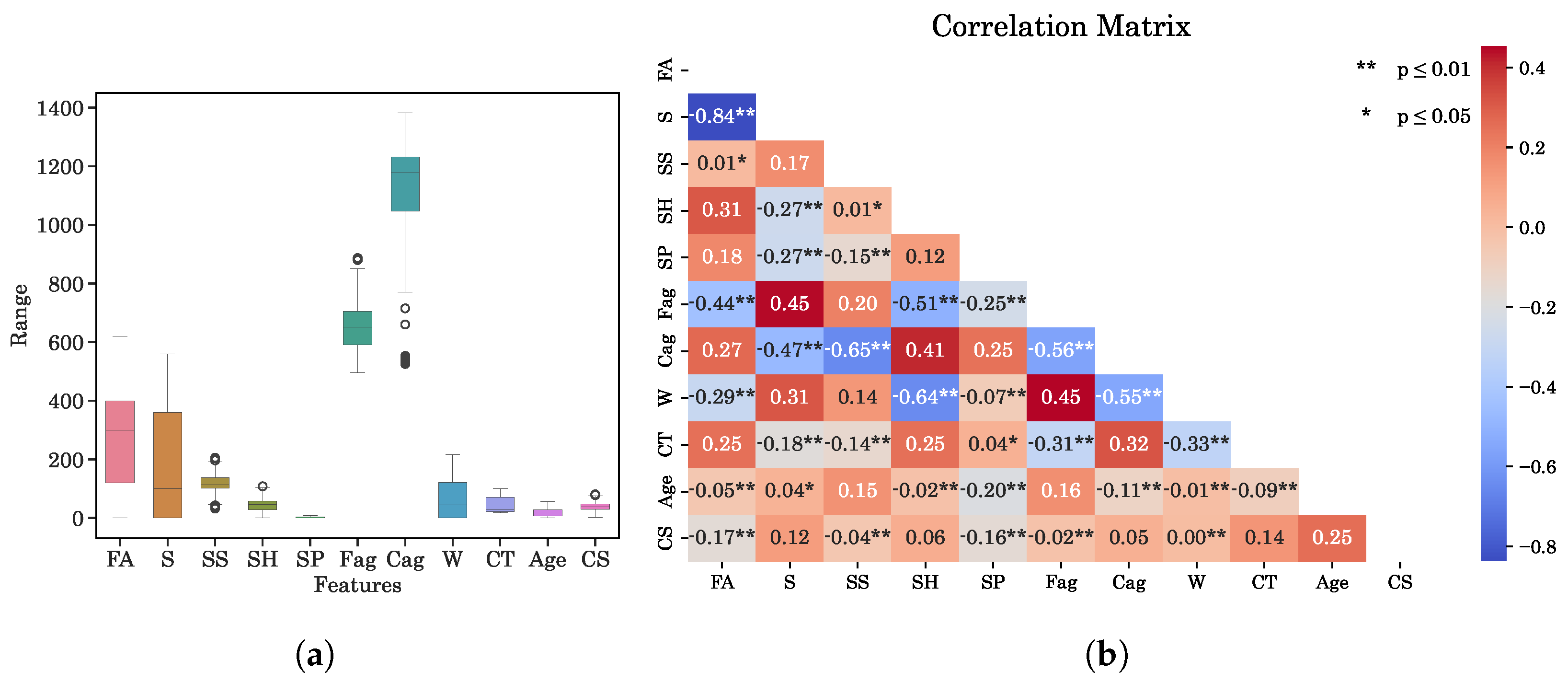
For the SP and CP parameters, the IQR was calculated, and any data point that fell outside the range of [Q1 − 1.5 × (IQR), Q3 + 1.5 × (IQR)] was identified as an outlier and removed from the dataset [61]. After removing the outliers from the SP and CP, the remaining data points in the dataset were used for further analysis and modeling. Figure 4a depicts the box plot of the dataset after outlier removal.

The Pearson correlation coefficients between all pairs of input parameters were calculated and illustrated in the correlation matrix shown in Figure 4b. The heatmap indicates that there are no parameters having strong linear relationship with each other. So, all the parameters are kept to construct the train and test datasets.

The statistical description of the dataset after outlier removal is presented in Table 3. The content of fly ash and GGBS varied significantly, with values ranging from 0 to 620 kg/m³ and 560 kg/m³, respectively. This wide range is attributed to the dataset including mixtures utilizing solely FA or GGBS, as well as combinations of both materials. The age of the concrete ranged from 1 to 56 days and the compressive strength ranged from 1.25 to 80.51 MPa.

In summary, the analysis of box plots, correlation heatmaps, and various statistical parameters reveals that the dataset contains few outliers and can accommodate all 10 input variables without multicollinearity issues. However, certain variables exhibit high skewness, indicating non-normal data distribution. This deviation from normality contradicts the assumptions of classical ML algorithms [62] like linear regression and Gaussian Naive Bayes. Therefore, the algorithms applied should be non-parameter algorithms or neural networks which do not explicitly assume that the input features (independent variables) are normally distributed or have a symmetric distribution [62].

4.2. Performance of Models before Data Augmentation

Figure 5 show the results of the three models (LightGBM, SVM, and CFNN) before data augmentation. The scatter plots in Figure 5a–c visually depict the models’ performance by comparing the predicted and observed values for both the training and test sets. Figure 5a demonstrates that LightGBM provides a moderate fit to the data. Figure 5b, which represents the SVM model, exhibits more scattered points that deviate further from the ideal line, indicating a poorer performance compared to LightGBM. Figure 5c, corresponding to the CFNN model, reveals that the data points are more tightly clustered around the ideal line, suggesting the best fit among the three models.

The time series plots in Figure 5d–f depict the tendency of the models in the test set. In Figure 5d, corresponding to the LightGBM model, the predicted values show some deviations from the observed values, indicating over- or underestimation tendencies for certain samples. Figure 5e, representing the SVM model, exhibits more pronounced deviations between the predicted and observed values, with noticeable over- or underestimation for some samples. Figure 5f, corresponding to the CFNN model, shows that the predicted values closely follow the observed values, suggesting minimal over- or underestimation tendencies across the test set samples.

Table 4. Model performance before data augmentation.

Model	Dataset	R2	MEA	RMSE	MAPE	RSR	WMAPE
LightGBM	Train	0.819	4.357	6.287	17.50%	0.409	11.067%
	Test	0.805	5.593	7.24	20.10%	0.600	14.921%
SVM	Train	0.893	3.945	5.277	26.00%	0.333	11.276%
	Test	0.783	4.918	7.309	22.00%	0.496	13.749%
CFNN	Train	0.902	2.973	3.348	6.00%	0.227	3.444%
	Test	0.842	3.940	6.442	18.00%	0.411	10.758%

provides an overview of the performance of models trained on the original dataset in predicting the compressive strength of geopolymer concrete. Accordingly, the CFNN model exhibited superior performance across all evaluation metrics. It achieved the highest $R^2$ values of 0.902 and 0.842 for the training and test sets, respectively. Additionally, the CFNN model had the lowest error values, with an MAE of 2.973 and 3.940, and an RMSE of 3.348 and 6.442 for the training and test sets, respectively. The CFNN model also demonstrated low percentage errors, with a MAPE of 6.00% for the training set and 18.00% for the test set. Furthermore, the RSR value of 0.411 for the test set suggests a relatively low standardized RMSE compared to the standard deviation of the measured data. The LightGBM model showed a reasonably good fit with $R^2$ values of 0.819 and 0.805 for the training and test sets, respectively. However, it exhibited higher error values, with an MAE of 4.357 and 5.593, and an RMSE of 6.287 and 7.24 for the training and test sets, respectively. The MAPE was 17.50% for the training set and 20.10% for the test set, suggesting relatively low percentage errors. The RSR value of 0.600 for the test set indicates a moderate standardized RMSE compared to the standard deviation of the measured data. Similarly, the SVM model displayed signs of overfitting, with a high $R^2$ of 0.893 on the training set but a lower value of 0.783 on the test set. Despite the lower $R^2$ on the test set, the model had lower MAE and RMSE values compared to LightGBM, with an MAE of 3.945 and 4.918, and an RMSE of 5.277 and 7.309 for the training and test sets, respectively. The MAPE was 26.00% for the training set and 22.00% for the test set, indicating low percentage errors. The RSR value of 0.496 for the test set suggests a relatively low standardized RMSE. Overall, the CFNN model demonstrated the most promising performance in predicting the compressive strength of geopolymer concrete among the models evaluated.

4.3. Synthetic Dataset

Table 5. Comparison of original and synthetic datasets.

Symbol	Unit	Mean		STD		Min		Max		Skewness
		Original	Synthetic	Original	Synthetic	Original	Synthetic	Original	Synthetic	Original	Synthetic
FA	kg/m3	246.72	238.01	159.99	150.28	0.00	0.00	620.00	546.91	−0.34	−0.20
GGBS	kg/m3	176.27	188.92	177.38	172.51	0.00	0.00	560.00	560.00	0.48	0.40
SS	kg/m3	117.56	119.44	36.08	36.01	32.00	33.11	205.50	203.66	0.23	0.23
SH	kg/m3	44.78	48.60	22.51	23.93	0.00	3.26	108.00	108.00	0.12	0.09
SP	kg/m3	1.52	1.69	2.57	2.54	0.00	0.00	9.00	8.33	1.35	1.13
fag	kg/m3	656.26	656.37	81.65	80.66	495.00	496.07	887.00	859.69	0.31	0.18
cag	kg/m3	1082.58	1063.82	239.87	246.23	525.40	528.40	1381.35	1351.08	−1.31	−1.08
w	kg/m3	64.72	70.93	62.10	60.39	0.00	0.00	216.00	212.41	0.47	0.29
CT	°C	48.16	49.90	28.21	28.09	19.00	19.00	100	100.00	0.50	0.41
CP	days	21.76	22.54	14.99	14.44	1.00	1.00	56	56.00	0.62	0.63
CS	MPa	38.45	35.05	14.95	16.48	1.25	0.00	80.51	80.51	0.13	0.12

demonstrates a statistical description of the synthetic compared to original data. The mean values of the features in the synthesized data closely approximated those of the original dataset, indicating that the TGAN model effectively captured the central tendencies inherent in the data. Additionally, the standard deviations exuded by the generalized data were compatible with those of the original data, subsuming that the TGAN model successfully replicated the disposition or variability present in the dataset. The examination of the minimum and maximum values of each feature further revealed that the range spread by the synthetic data aligned well with that of the original data, ensuring that the synthetic data does not contain any unrealistic outliers or values outside the valid range. Furthermore, skewness, a measure of asymmetry in the distributions, was highly similar between the two datasets, indicating that the TGAN model retained the shape characteristics of the original data distributions. The fact that the mean, standard deviation, minimum, maximum, and skewness values of the features in the synthetic data are effectively the same as those of the original data suggests that the generated data points capture the key statistical properties and patterns present in the real dataset.

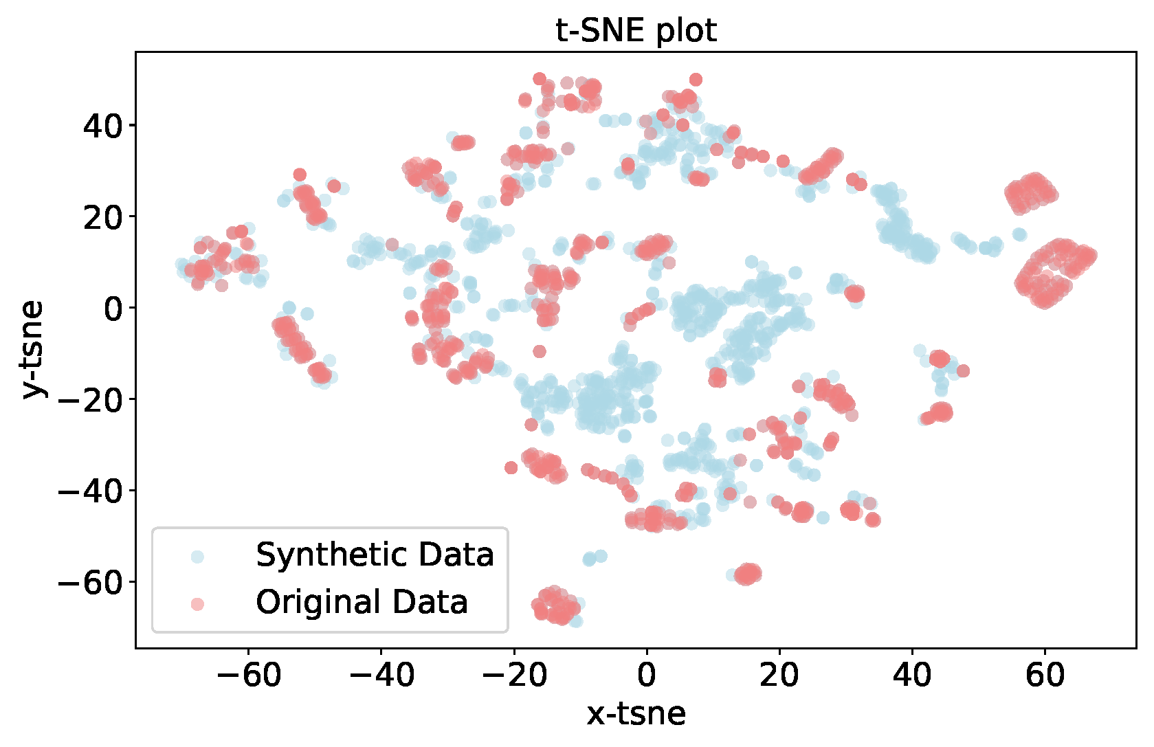
Figure 6 presents a t-SNE plot comparing the original data and the synthetic data generated by the TGAN model. The t-SNE algorithm is a dimensionality reduction technique that projects high-dimensional data into a lower-dimensional space (in this case, a 2D plane) while preserving the local structure and relationships between data points [11]. In the t-SNE plot, each data point is represented as a colored dot, with the original data points shown in one color (e.g., blue) and the synthetic data points generated by the TGAN model shown in another color (e.g., orange). The proximity of the data points in the plot indicates their similarity in the high-dimensional feature space. The t-SNE plot shows that the synthetic data points generated by the TGAN model are well-distributed and intermixed with the original data points. This suggests that the TGAN model has successfully captured the underlying patterns and distributions present in the original data, and the generated synthetic data points share similar characteristics and relationships with the real data points.

The ability of the TGAN model to generate high-quality synthetic data is crucial for data augmentation techniques, as it can help increase the size and diversity of the training dataset without introducing unrealistic or inconsistent data points. By generating 1000 additional data points using the TGAN model, the total training dataset size has been increased, potentially improving the performance and generalization capabilities of the ML models trained on this augmented dataset.

4.4. Performance of Models after Data Augmentation

The data augmentation approach using the tabular GAN to generate synthetic samples led to substantial improvements in the predictive performance of all three models, as evidenced by Figure 7. The scatter plots show that the data points representing the predicted versus observed compressive strength values lie much closer to the ideal line after augmentation, indicating a stronger agreement between predictions and observations across the entire data range. The LightGBM and SVM models also exhibit improved performance with reduced scatter compared to their pre-augmentation results; their predictions still deviate more from the ideal line, particularly for higher strength values. For the CFNN model, the augmented data enabled the model to learn more robust patterns. This suggests that the CFNN model benefited more from the augmented data in capturing the underlying complexities and nuances of the problem.

The tendency plots in Figure 7d–f further corroborate these observations. For the CFNN, the predicted values closely track the actual observed values across the entire test set, with minimal discrepancies on a sample-by-sample basis. In contrast, the LightGBM and SVM models, while improved, still exhibit noticeable fluctuations and deviations from the observed values, indicating a higher propensity for over- or underestimation on certain test samples.

Also, the performance of the models is demonstrated in more detail in

Table 6. Model performance.

Model	Dataset	R2	MAE	RMSE	MAPE	RSR	WMAPE
LightGBM	Train	0.913	3.004	4.676	10.00%	0.282	7.679%
	Test	0.877	3.366	4.657	10.32%	0.413	9.413%
SVM	Train	0.922	2.373	4.256	12.00%	0.281	4.323%
	Test	0.863	2.897	4.61	21.00%	0.399	5.757%
CFNN	Train	0.956	1.037	2.982	18.10%	0.181	2.717%
	Test	0.942	1.546	3.836	22.83%	0.194	3.265%

. Overall, the models achieved better performance after data augmentation. The CFNN model exhibited substantial improvements across all metrics after data augmentation. The $R^2$ increased from 0.902 to 0.956 on the training set and 0.842 to 0.942 on the test set, indicating better explained variance and goodness of fit. The MAE decreased from 2.973 to 1.037 MPa on the training set and 3.940 to 1.546 MPa on the test set, representing reductions of 65.12% and 60.74% respectively. Similarly, the RMSE dropped from 3.348 to 2.982 MPa on the training set (10.9% reduction) and 6.442 to 3.836 MPa on the test set (40.5% reduction). The MAPE saw a notable decrease from 6.00% to 18.10% on the training set, though it improved from 18.00% to 5.283% on the test set. The RSR also reduced from 0.227 to 0.181 on the training set and 0.411 to 0.194 on the test set, indicating smaller errors relative to data variability. Overall, the CFNN demonstrated consistent and substantial improvements across all metrics after augmentation.

For LightGBM, the $R^2$ increased from 0.819 to 0.913 on the training set and 0.805 to 0.877 on the test set after augmentation. The MAE decreased from 4.357 to 3.004 MPa (31.1% reduction) on the training set and 5.593 to 3.366 MPa (39.9% reduction) on the test set. The RMSE also saw improvements, dropping from 6.287 to 4.676 MPa (25.7% reduction) on the training set and 7.240 to 4.657 MPa (35.6% reduction) on the test set. The MAPE decreased from 0.175% to 0.1% on the training set and 0.201% to 0.10% on the test set. Lastly, the RSR improved from 0.409 to 0.282 on the training set and 0.600 to 0.413 on the test set. While LightGBM showed improvements across all metrics, the magnitude of improvement was generally smaller compared to the CFNN model.

The SVM model also benefited from data augmentation, with the $R^2$ increasing from 0.893 to 0.922 on the training set and 0.783 to 0.863 on the test set. The MAE improved from 3.945 to 1.373 MPa (39.9% reduction) on the training set and 4.918 to 2.897 MPa (41.1% reduction) on the test set. The RMSE decreased from 5.277 to 3.256 MPa (38.2% reduction) on the training set and 7.309 to 5.61 MPa (23.2% reduction) on the test set. The MAPE remained relatively unchanged at 0.06% on the training set but improved from 0.18% to 0.21% on the test set. Finally, the RSR saw improvements, decreasing from 0.333 to 0.281 on the training set and 0.411 to 0.399 on the test set.

4.5. Discussion and Limitations

The comparison of model performance before and after data augmentation is visualized in Figure 8. The findings align with relevant studies that have utilized synthetic data for ML models in predicting the compressive strength of concrete [11,13]. Research conducted by Chen et al. (2022) [11] highlights the effectiveness of integrating synthetic data, showcasing a significant improvement in the accuracy of deep learning models (i.e., CNNs), compared to traditional ML models. Similarly, this study underscores the efficacy of data augmentation methods in enhancing model predictive capabilities, particularly for CFNNs, despite the inherent variability in precursor chemicals. Additionally, the results suggest that the implementation of data augmentation techniques for SVMs leads to more substantial improvements compared to tree-based models, although the distinction may not be immediately apparent. While the use of synthetic data has proven effective in enhancing the performance of the LightGBM and CFNN models, as evidenced by the improvements in metrics such as MAE, RMSE, RSR, and WMAPE, its impact on the MAPE of the SVM model remains limited. This can be attributed to the inherent sensitivity of SVM models to the presence of outliers in the dataset [63]. Consequently, the outliers observed in the coarse aggregate and fine aggregate features may have adversely influenced the SVM model’s performance relative to the LightGBM and CFNN models.

Notwithstanding the observed enhancements in model performance, it is crucial to acknowledge that the generation of synthetic data in this study does not necessarily augment the generalizability of the models. As demonstrated in Table 5, the minimum, maximum, and skewness values of the synthetic data are either reduced or maintained at the same level as the original dataset. However, it is worth noting that generating data with broader coverage may potentially introduce model uncertainty due to extrapolation, thus necessitating further investigation to assess the trade-offs between model performance and generalizability.

Despite the high performance in the test set, it should be noted that the test set and training set in this study are constructed using the same dataset obtained from open literature. This can cause overoptimistic performance estimates because the data distribution in both sets is identical. Additionally, it is important to consider that data sourced from previous studies may not always be reliable and the presence of measurement biases among multiple studies further adds to the uncertainty of prediction outcomes. Moreover, the data collected in this study is confined to specific countries and regions, notably China, India, Iran, and Australia, where geopolymer research has received considerable attention. Consequently, the dataset lacks comprehensive international representation, thereby limiting its scope and exhaustiveness.

To interpret the developed model effectively, permutation feature importance and SHapley Additive exPlanations (SHAP) were adopted, shedding light on the intricate interplay between input features and their influence on compressive strength. These two interpretability techniques were conducted within CFNNs, recognized as the most promising model. Permutation feature importance evaluates the variation in prediction error resulting from the permutation of feature values. If prediction error remains unchanged after shuffling values, the feature is considered ’unimportant,’ signifying the model’s disregard for it in prediction. This approach offers a concise, comprehensive understanding of the model’s behavior. SHAP, grounded in coalitional game theory, conceptualize prediction as a game, with features akin to players. The SHAP value assigned to each feature delineates its average marginal contribution across all conceivable coalitions, thereby elucidating its impact on attaining a heightened or diminished final prediction outcome.

Figure 9 presents the overall importance of the features. The most influential features for predicting compressive strength are the specimen age and curing temperature, with permutation importance of 0.38 and 0.35, respectively. Similar results were observed in the SHAP analysis, with slight discrepancies in the influence of slag and fine aggregate content between the two analyses. SHAP analysis presents that higher slag content generally results in increased compressive strength, denoted by the prominent red coloring on the right side of the slag feature. Conversely, higher fly ash content tends to have a detrimental effect on compressive strength, as evidenced by the pink coloring on the right side of the fly ash feature. The impact of fine aggregate content is more nuanced, with both positive and negative effects depending on the specific value of the feature. Other features, such as sodium hydroxide, water content, coarse aggregate, and sodium silicate, exhibit relatively smaller impacts on compressive strength prediction, as indicated by their narrower ranges of SHAP values and lower permutation importance. Superplasticizer content demonstrates a significantly smaller influence compared to the other features (permutation importance = 0.02).

It can be observed that that variables of specimen age and curing temperature are the most important features in the decision making of the CFNN model. These factors are expressed in integers and have a high frequency of repetition according to the curing regime. Therefore, the TGAN model can capture features and generate better data. Meanwhile, factors with many outliers such as superplasticizer and coarse aggregate are the least influential features. These may be the reasons why the CFNN model benefits a lot from synthetic data. Additionally, a study conducted by Rahmati et al. (2022) [64] highlights the impact of curing time and curing method (i.e., oven, steam) on the prediction of ML models. However, these factors were not considered in the current study due to the problem of high dimensionality associated with the complexity of the dataset. Incorporating these factors with larger datasets can improve the accuracy of the prediction model.

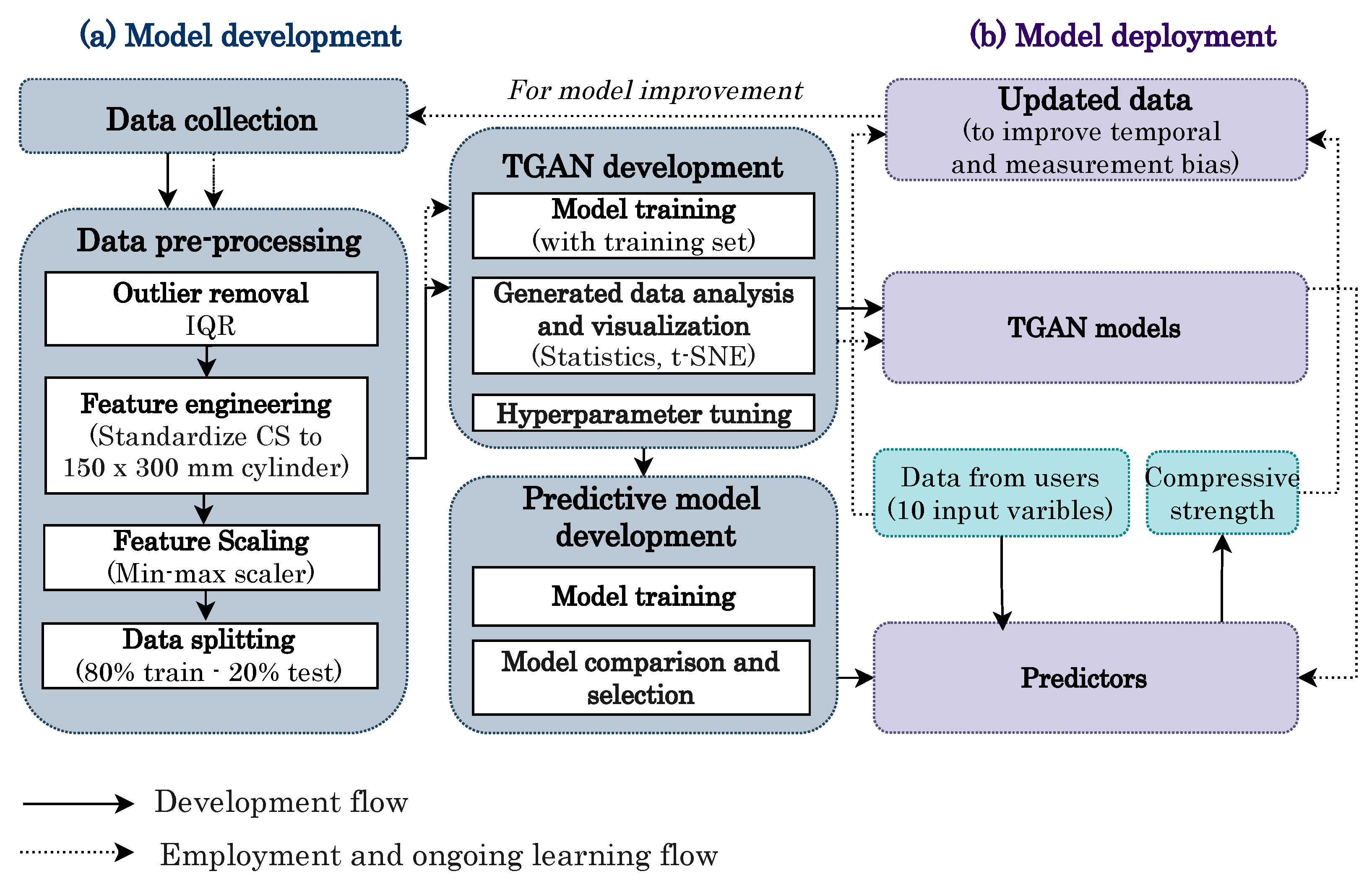
Considering model characteristics and limitations, a process for deploying and enhancing models was proposed in Figure 10. The developed TGAN and predictive models can be refined using real data from users labeled with the prediction results. The effectiveness of using the results of the ML model to further improve the model is demonstrated in the research of Ford et al. (2022) [61]. This ongoing learning process ensures that the deployed models can enhance generalization and mitigate temporal and measurement uncertainties, ultimately improving their performance and reliability over time.

5. Conclusions and Future Works

This study examines the impact of using synthetic data on ML models that predict the compressive strength of geopolymer concrete. For this purpose, 930 data points were collected from the open literature. The TGAN method was employed to generate geopolymer mixture and compressive strength data. The ML model consists of LightGBM, SVM, and CFNN algorithms, representing tree-based, support vector, and neural network algorithms, respectively. These models were trained using the generated data and subsequently evaluated using the real dataset. A comparison was made with the corresponding model using the original dataset. Based on the obtained results, the following conclusions can be drawn:

• TGAN proves capable of generating mixture and compressive strength data for geopolymer concrete. The synthetic data significantly improves the performance of ML models, as evident from the increased R² values and reduced error indices such as MAE, RMSE, MAPE, RSR, and WMAPE. The CFNN model exhibited the most improvement, followed by LightGBM and SVM.
• The enhanced performance of the models indicates that the heterogeneity in the type or quality of precursors in the collected data does not significantly affect the data generation ability and performance of ML models.
• Due to the presence of numerous outliers and skewed characteristics of the data, the SVM model was greatly impacted in both the original and synthetic datasets.
• The generated data statistics demonstrate that the characteristics of the data are quite similar to the original data. This indicates that the TGAN model generated reliable data. However, it is important to note that using such data merely improves accuracy without enhancing the generalization capabilities of the models.
• In addition, this study demonstrates limitations concerning the generalizability of the model, the scope of inputs, the absence of validation with actual experimental data, and regional bias within the dataset.

Several avenues for future research can be pursued to address the limitations identified in this study. Firstly, prioritizing exploration of generator architectures within GANs or employing of bounded GANs could enable better control over the range of generated data. Furthermore, the generalization capability of the models can be enhanced through the implementation of regularization techniques (e.g., dropout, and L1 and L2 regularization), cross-validation, and the adaptation of open-source algorithms tailored to the characteristics of the data. Instead of solely relying on integration algorithms, future research should focus on enhancing existing algorithms to better align with the characteristics of data. To assess practical effectiveness, the developed TGAN and predictive models necessitate further verification through experimental data or real-world project implementation. Moreover, expanding the scope of input variables, such as the chemical and physical composition of precursors, curing duration, and methodologies, could potentially improve the predictive accuracy of the models. Expanding the dataset to include geopolymer research across diverse regions and countries also serves to enhance the internationality and generalizability of the model. The aggregation of a comprehensive dataset holds promise for broadening the scope of output variables to encompass additional mechanical properties, including tensile strength, flexural strength, durability, and the effects of aging on geopolymer concrete.

References

- Habert, G.; Miller, S.A.; John, V.M.; Provis, J.L.; Favier, A.; Horvath, A.; Scrivener, K.L. Environmental impacts and decarbonization strategies in the cement and concrete industries. Nat. Rev. Earth Environ. 2020, 1, 559–573. [Google Scholar] [CrossRef]
- Nwankwo, C.O.; Bamigboye, G.O.; Davies, I.E.; Michaels, T.A. High volume Portland cement replacement: A review. Constr. Build. Mater. 2020, 260, 120445. [Google Scholar] [CrossRef]
- Scrivener, K.L.; John, V.M.; Gartner, E.M. Eco-efficient cements: Potential economically viable solutions for a low-CO2 cement-based materials industry. Cem. Concr. Res. 2018, 114, 2–26. [Google Scholar] [CrossRef]
- Zhuang, X.Y.; Chen, L.; Komarneni, S.; Zhou, C.H.; Tong, D.S.; Yang, H.M.; Yu, W.H.; Wang, H. Fly ash-based geopolymer: Clean production, properties and applications. J. Clean. Prod. 2016, 125, 253–267. [Google Scholar] [CrossRef]
- Zakka, W.P.; Lim, N.H.A.S.; Khun, M.C. A scientometric review of geopolymer concrete. J. Clean. Prod. 2021, 280, 124353. [Google Scholar] [CrossRef]
- Dwibedy, S.; Panigrahi, S.K. Factors affecting the structural performance of geopolymer concrete beam composites. Constr. Build. Mater. 2023, 409, 134129. [Google Scholar] [CrossRef]
- Li, N.; Shi, C.; Zhang, Z.; Wang, H.; Liu, Y. A review on mixture design methods for geopolymer concrete. Compos. Part B Eng. 2019, 178, 107490. [Google Scholar] [CrossRef]
- Gupta, T.; Rao, M.C. Prediction of compressive strength of geopolymer concrete using machine learning techniques. Struct. Concr. 2022, 23, 3073–3090. [Google Scholar] [CrossRef]
- Li, Z.; Yoon, J.; Zhang, R.; Rajabipour, F.; Srubar III, W.V.; Dabo, I.; Radlińska, A. Machine learning in concrete science: Applications, challenges, and best practices. npj Comput. Mater. 2022, 8, 127. [Google Scholar] [CrossRef]
- Yasuno, T.; Nakajima, M.; Sekiguchi, T.; Noda, K.; Aoyanagi, K.; Kato, S. Synthetic image augmentation for damage region segmentation using conditional GAN with structure edge. arXiv 2020, arXiv:2005.08628. [Google Scholar]
- Chen, N.; Zhao, S.; Gao, Z.; Wang, D.; Liu, P.; Oeser, M.; Hou, Y.; Wang, L. Virtual mix design: Prediction of compressive strength of concrete with industrial wastes using deep data augmentation. Constr. Build. Mater. 2022, 323, 126580. [Google Scholar] [CrossRef]
- Liu, K.H.; Xie, T.Y.; Cai, Z.K.; Chen, G.M.; Zhao, X.Y. Data-driven prediction and optimization of axial compressive strength for FRP-reinforced CFST columns using synthetic data augmentation. Eng. Struct. 2024, 300, 117225. [Google Scholar] [CrossRef]
- Marani, A.; Jamali, A.; Nehdi, M.L. Predicting ultra-high-performance concrete compressive strength using tabular generative adversarial networks. Materials 2020, 13, 4757. [Google Scholar] [CrossRef] [PubMed]
- Sharma, U.; Gupta, N.; Verma, M. Prediction of the compressive strength of Flyash and GGBS incorporated geopolymer concrete using artificial neural network. Asian J. Civ. Eng. 2023, 24, 2837–2850. [Google Scholar] [CrossRef]
- Gupta, P.; Gupta, N.; Goyal, S. Predicting compressive strength of calcined clay, fly ash-based geopolymer composite using supervised learning algorithm. Adv. Appl. Math. Sci. 2022, 21, 4151–4161. [Google Scholar]
- Jafari, A.; Toufigh, V. Developing a comprehensive prediction model for the compressive strength of slag-based alkali-activated concrete. J. Sustain. Cem.-Based Mater. 2024, 13, 256–273. [Google Scholar] [CrossRef]
- Kumar, P.; Pratap, B.; Sharma, S.; Kumar, I. Compressive strength prediction of fly ash and blast furnace slag-based geopolymer concrete using convolutional neural network. Asian J. Civ. Eng. 2024, 25, 1561–1569. [Google Scholar] [CrossRef]
- Huynh, A.T.; Nguyen, Q.D.; Xuan, Q.L.; Magee, B.; Chung, T.; Tran, K.T.; Nguyen, K.T. A machine learning-assisted numerical predictor for compressive strength of geopolymer concrete based on experimental data and sensitivity analysis. Appl. Sci. 2020, 10, 7726. [Google Scholar] [CrossRef]
- Wang, Q.; Ahmad, W.; Ahmad, A.; Aslam, F.; Mohamed, A.; Vatin, N.I. Application of soft computing techniques to predict the strength of geopolymer composites. Polymers 2022, 14, 1074. [Google Scholar] [CrossRef]
- Tran, V.Q. Data-driven approach for investigating and predicting of compressive strength of fly ash–slag geopolymer concrete. Struct. Concr. 2023, 24, 7419–7444. [Google Scholar] [CrossRef]
- Ahmed, H.U.; Mohammed, A.S.; Mohammed, A.A. Proposing several model techniques including ANN and M5P-tree to predict the compressive strength of geopolymer concretes incorporated with nano-silica. Environ. Sci. Pollut. Res. 2022, 29, 71232–71256. [Google Scholar] [CrossRef] [PubMed]
- Nazar, S.; Yang, J.; Amin, M.N.; Khan, K.; Ashraf, M.; Aslam, F.; Javed, M.F.; Eldin, S.M. Machine learning interpretable-prediction models to evaluate the slump and strength of fly ash-based geopolymer. J. Mater. Res. Technol. 2023, 24, 100–124. [Google Scholar] [CrossRef]
- Ahmed, H.U.; Mostafa, R.R.; Mohammed, A.; Sihag, P.; Qadir, A. Support vector regression (SVR) and grey wolf optimization (GWO) to predict the compressive strength of GGBFS-based geopolymer concrete. Neural Comput. Appl. 2023, 35, 2909–2926. [Google Scholar] [CrossRef]
- Kumar, A.; Arora, H.C.; Kapoor, N.R.; Kumar, K. Prognosis of compressive strength of fly-ash-based geopolymer-modified sustainable concrete with ML algorithms. Struct. Concr. 2023, 24, 3990–4014. [Google Scholar] [CrossRef]
- Ahmed, H.U.; Mohammed, A.A.; Mohammed, A. Soft computing models to predict the compressive strength of GGBS/FA-geopolymer concrete. PLoS ONE 2022, 17, e0265846. [Google Scholar] [CrossRef] [PubMed]
- Gunasekara, C.; Lokuge, W.; Keskic, M.; Raj, N.; Law, D.; Setunge, S. Design of alkali-activated slag-fly ash concrete mixtures using machine learning. Mater. J. 2020, 117, 263–278. [Google Scholar]
- Gogineni, A.; Panday, I.K.; Kumar, P.; Paswan, R.k. Predictive modelling of concrete compressive strength incorporating GGBS and alkali using a machine-learning approach. Asian J. Civ. Eng. 2024, 25, 699–709. [Google Scholar] [CrossRef]
- Nukah, P.D.; Abbey, S.J.; Booth, C.A.; Oti, J. Evaluation of the structural performance of low carbon concrete. Sustainability 2022, 14, 16765. [Google Scholar] [CrossRef]
- Kina, C.; Tanyildizi, H.; Turk, K. Forecasting the compressive strength of GGBFS-based geopolymer concrete via ensemble predictive models. Constr. Build. Mater. 2023, 405, 133299. [Google Scholar] [CrossRef]
- Parhi, S.K.; Panigrahi, S.K. Alkali–silica reaction expansion prediction in concrete using hybrid metaheuristic optimized machine learning algorithms. Asian J. Civ. Eng. 2024, 25, 1091–1113. [Google Scholar] [CrossRef]
- Dunphy, K.; Fekri, M.N.; Grolinger, K.; Sadhu, A. Data augmentation for deep-learning-based multiclass structural damage detection using limited information. Sensors 2022, 22, 6193. [Google Scholar] [CrossRef] [PubMed]
- Goodfellow, I.; Pouget-Abadie, J.; Mirza, M.; Xu, B.; Warde-Farley, D.; Ozair, S.; Courville, A.; Bengio, Y. Generative adversarial nets. Adv. Neural Inf. Process. Syst. 2014, 27, 2672–2680. [Google Scholar]
- Jia, J.F.; Chen, X.Z.; Bai, Y.L.; Li, Y.L.; Wang, Z.H. An interpretable ensemble learning method to predict the compressive strength of concrete. Structures 2022, 46, 201–213. [Google Scholar] [CrossRef]
- Çalışkan, A.; Demirhan, S.; Tekin, R. Comparison of different machine learning methods for estimating compressive strength of mortars. Constr. Build. Mater. 2022, 335, 127490. [Google Scholar] [CrossRef]
- Hasanipanah, M.; Jamei, M.; Mohammed, A.S.; Amar, M.N.; Hocine, O.; Khedher, K.M. Intelligent prediction of rock mass deformation modulus through three optimized cascaded forward neural network models. Earth Sci. Inform. 2022, 15, 1659–1669. [Google Scholar] [CrossRef]
- Mijwel, M.M. Artificial neural networks advantages and disadvantages. Mesopotamian J. Big Data 2021, 2021, 29–31. [Google Scholar] [CrossRef]
- Sun, L.; Koopialipoor, M.; Jahed Armaghani, D.; Tarinejad, R.; Tahir, M. Applying a meta-heuristic algorithm to predict and optimize compressive strength of concrete samples. Eng. Comput. 2021, 37, 1133–1145. [Google Scholar] [CrossRef]
- Liang, M.; Chang, Z.; Wan, Z.; Gan, Y.; Schlangen, E.; Šavija, B. Interpretable Ensemble-Machine-Learning models for predicting creep behavior of concrete. Cem. Concr. Compos. 2022, 125, 104295. [Google Scholar] [CrossRef]
- Ling, H.; Qian, C.; Kang, W.; Liang, C.; Chen, H. Combination of Support Vector Machine and K-Fold cross validation to predict compressive strength of concrete in marine environment. Constr. Build. Mater. 2019, 206, 355–363. [Google Scholar] [CrossRef]
- Pwasong, A.; Sathasivam, S. A new hybrid quadratic regression and cascade forward backpropagation neural network. Neurocomputing 2016, 182, 197–209. [Google Scholar] [CrossRef]
- Joseph, B.; Mathew, G. Influence of aggregate content on the behavior of fly ash based geopolymer concrete. Sci. Iran. 2012, 19, 1188–1194. [Google Scholar] [CrossRef]
- Nath, P.; Sarker, P.K. Effect of GGBFS on setting, workability and early strength properties of fly ash geopolymer concrete cured in ambient condition. Constr. Build. Mater. 2014, 66, 163–171. [Google Scholar] [CrossRef]
- Vora, P.R.; Dave, U.V. Parametric studies on compressive strength of geopolymer concrete. Procedia Eng. 2013, 51, 210–219. [Google Scholar] [CrossRef]
- Demie, S.; Nuruddin, M.F.; Shafiq, N. Effects of micro-structure characteristics of interfacial transition zone on the compressive strength of self-compacting geopolymer concrete. Constr. Build. Mater. 2013, 41, 91–98. [Google Scholar] [CrossRef]
- Lee, N.; Lee, H.K. Setting and mechanical properties of alkali-activated fly ash/slag concrete manufactured at room temperature. Constr. Build. Mater. 2013, 47, 1201–1209. [Google Scholar] [CrossRef]
- Nuaklong, P.; Sata, V.; Chindaprasirt, P. Influence of recycled aggregate on fly ash geopolymer concrete properties. J. Clean. Prod. 2016, 112, 2300–2307. [Google Scholar] [CrossRef]
- Rajarajeswari, A.; Dhinakaran, G. Compressive strength of GGBFS based GPC under thermal curing. Constr. Build. Mater. 2016, 126, 552–559. [Google Scholar] [CrossRef]
- Su, H.; Xu, J.; Ren, W. Mechanical properties of geopolymer concrete exposed to dynamic compression under elevated temperatures. Ceram. Int. 2016, 42, 3888–3898. [Google Scholar] [CrossRef]
- Tennakoon, C.; Shayan, A.; Sanjayan, J.G.; Xu, A. Chloride ingress and steel corrosion in geopolymer concrete based on long term tests. Mater. Des. 2017, 116, 287–299. [Google Scholar] [CrossRef]
- Wardhono, A.; Gunasekara, C.; Law, D.W.; Setunge, S. Comparison of long term performance between alkali activated slag and fly ash geopolymer concretes. Constr. Build. Mater. 2017, 143, 272–279. [Google Scholar] [CrossRef]
- Reddy, M.S.; Dinakar, P.; Rao, B.H. Mix design development of fly ash and ground granulated blast furnace slag based geopolymer concrete. J. Build. Eng. 2018, 20, 712–722. [Google Scholar] [CrossRef]
- Nguyen, K.T.; Le, T.A.; Lee, K. Evaluation of the mechanical properties of sea sand-based geopolymer concrete and the corrosion of embedded steel bar. Constr. Build. Mater. 2018, 169, 462–472. [Google Scholar] [CrossRef]
- Li, N.; Shi, C.; Zhang, Z.; Zhu, D.; Hwang, H.J.; Zhu, Y.; Sun, T. A mixture proportioning method for the development of performance-based alkali-activated slag-based concrete. Cem. Concr. Compos. 2018, 93, 163–174. [Google Scholar] [CrossRef]
- Nagaraj, V.K.; Venkatesh Babu, D.L. Assessing the performance of molarity and alkaline activator ratio on engineering properties of self-compacting alkaline activated concrete at ambient temperature. J. Build. Eng. 2018, 20, 137–155. [Google Scholar]
- Morsy, A.M.; Ragheb, A.M.; Shalan, A.H.; Mohamed, O.H. Mechanical characteristics of GGBFS/FA-based geopolymer concrete and its environmental impact. Pract. Period. Struct. Des. Constr. 2022, 27, 04022017. [Google Scholar] [CrossRef]
- Gunasekera, C.; Setunge, S.; Law, D.W. Correlations between mechanical properties of low-calcium fly ash geopolymer concretes. J. Mater. Civ. Eng. 2017, 29, 04017111. [Google Scholar] [CrossRef]
- Sukmak, P.; Horpibulsuk, S.; Shen, S.L. Strength development in clay–fly ash geopolymer. Constr. Build. Mater. 2013, 40, 566–574. [Google Scholar] [CrossRef]
- Somna, K.; Jaturapitakkul, C.; Kajitvichyanukul, P.; Chindaprasirt, P. NaOH-activated ground fly ash geopolymer cured at ambient temperature. Fuel 2011, 90, 2118–2124. [Google Scholar] [CrossRef]
- Suksiripattanapong, C.; Horpibulsuk, S.; Chanprasert, P.; Sukmak, P.; Arulrajah, A. Compressive strength development in fly ash geopolymer masonry units manufactured from water treatment sludge. Constr. Build. Mater. 2015, 82, 20–30. [Google Scholar] [CrossRef]
- Talaat, A.; Emad, A.; Tarek, A.; Masbouba, M.; Essam, A.; Kohail, M. Factors affecting the results of concrete compression testing: A review. Ain Shams Eng. J. 2021, 12, 205–221. [Google Scholar] [CrossRef]
- Taffese, W.Z.; Abegaz, K.A. Prediction of compaction and strength properties of amended soil using machine learning. Buildings 2022, 12, 613. [Google Scholar] [CrossRef]
- Benavoli, A.; Corani, G.; Mangili, F. Should we really use post-hoc tests based on mean-ranks? J. Mach. Learn. Res. 2016, 17, 152–161. [Google Scholar]
- Chowdhary, C.L.; Mittal, M.; P, K.; Pattanaik, P.A.; Marszalek, Z. An efficient segmentation and classification system in medical images using intuitionist possibilistic fuzzy C-mean clustering and fuzzy SVM algorithm. Sensors 2020, 20, 3903. [Google Scholar] [CrossRef] [PubMed]
- Rahmati, M.; Toufigh, V. Evaluation of geopolymer concrete at high temperatures: An experimental study using machine learning. J. Clean. Prod. 2022, 372, 133608. [Google Scholar] [CrossRef]
Figure 1.
TGAN model in this study.
Figure 2.
CFNN architecture in this study.
Figure 3.
Evaluation flowchart of data augmentation and predictive models.
Figure 4.
Data analysis. (a) Box plot after outlier removal. (b) Correlation matrix.
Figure 5.
Model performance before data augmentation.
Figure 6.
t-SNE visualization of the synthetic and original data.
Figure 7.
Model performance after data augmentation.
Figure 8.
Comparison of R2 and error indices of the models before and after data augmentation.
Figure 9.
The importance of each feature of CFNN model. (a) Permutation importance. (b) SHAP value.
Figure 10.
Schematic diagram of model deployment and improvement process.