
A Robust Methodology for Dynamic Proximity Sensing of Vehicles Overtaking Micromobility Devices in a Noisy Environment

Abstract
:1. Introduction
2. Methodology
3. Sensor Selection
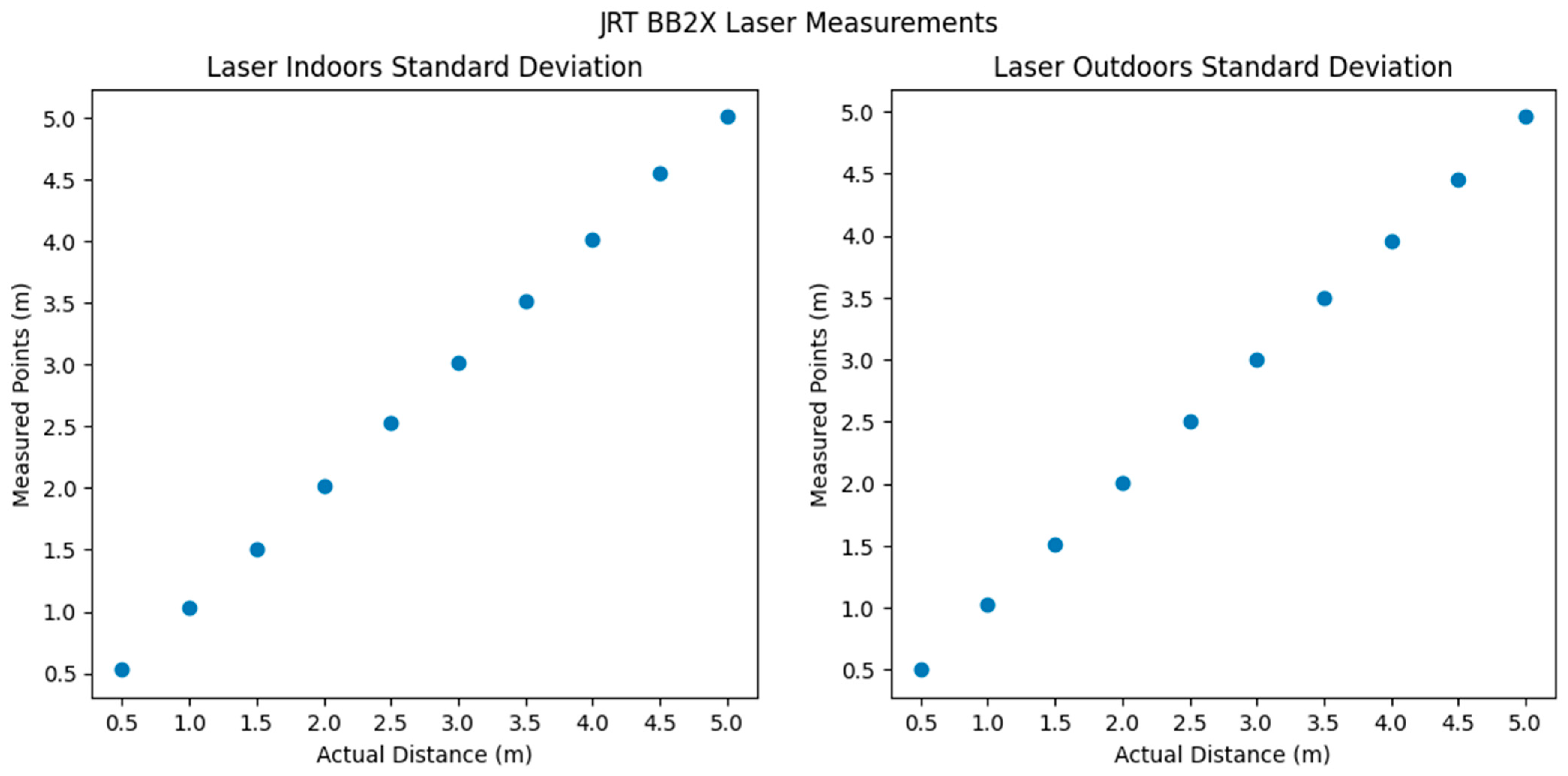
3.1. Indoor and Outdoor Fixed Distance Tests
3.2. Stationary Bike Test
3.2.1. Laser Sensor
3.2.2. LiDAR Sensor
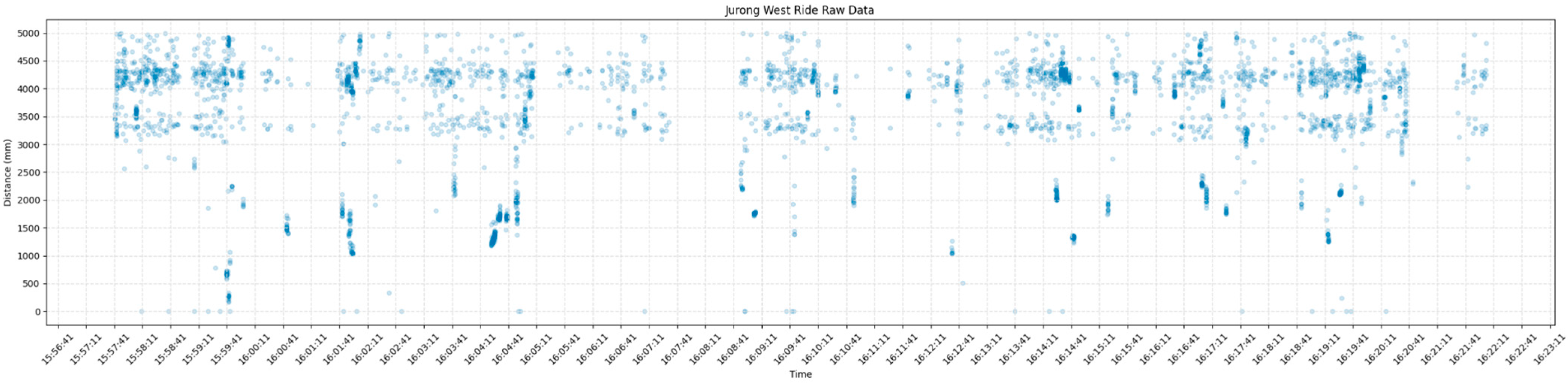
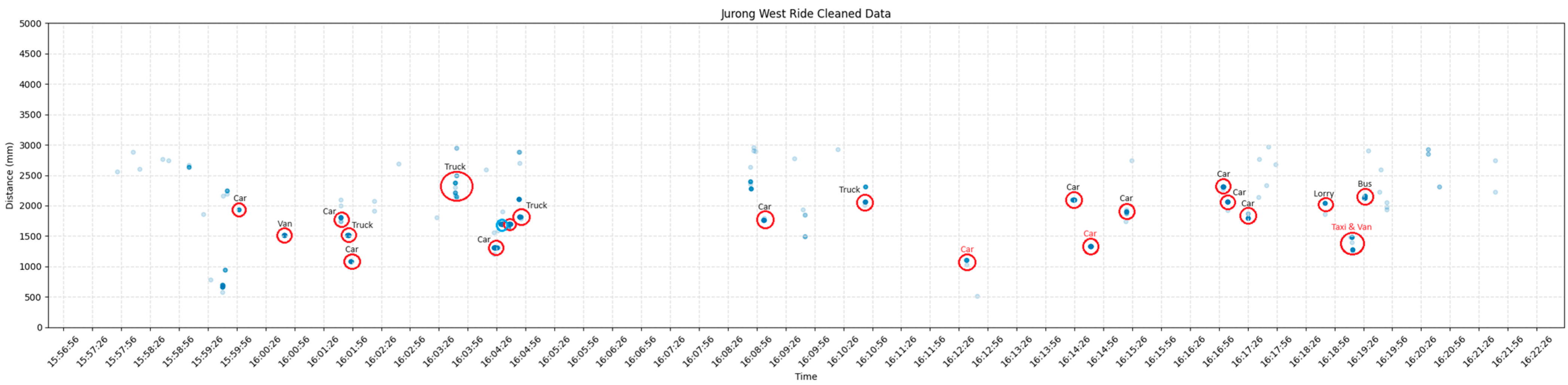
4. Mobile Bike Test
4.1. Setup
4.2. Preliminary Results
4.3. Automated Data Analysis
4.3.1. Clustering Algorithm Selection
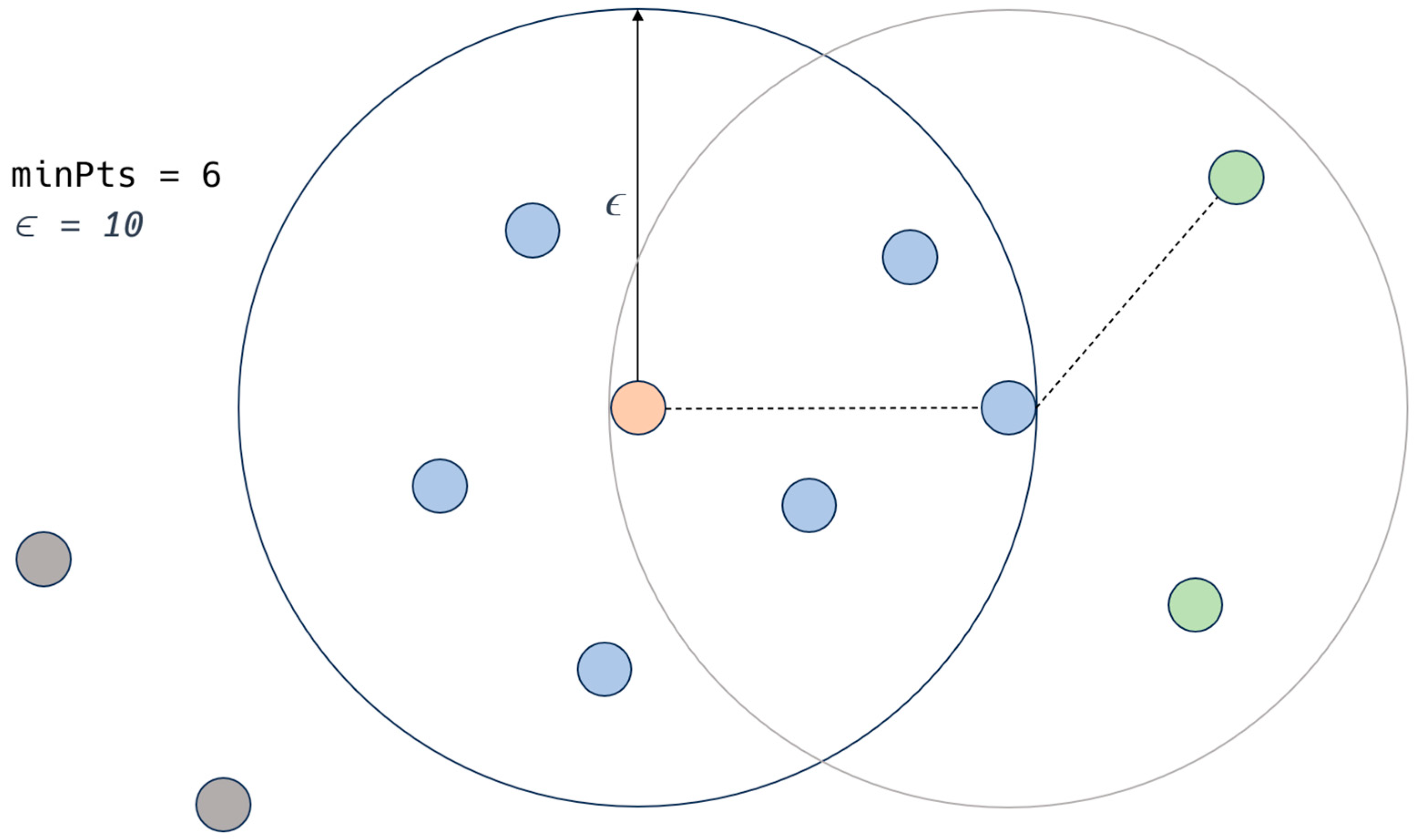
4.3.2. DBSCAN
- For any two points and in , if is reachable from , then and are part of the same cluster.
- For any point in , if there is a point in such that is reachable from , and is a core point.
5. Speed Considerations
6. Limitations and Future Work
7. Conclusions
Author Contributions
Funding
Institutional Review Board Statement
Informed Consent Statement
Data Availability Statement
Conflicts of Interest
References
- De Hartog, J.J.; Boogaard, H.; Nijland, H.; Hoek, G. Do the Health Benefits of Cycling Outweigh the Risks? Environ. Health Perspect. 2010, 118, 1109–1116. [Google Scholar] [CrossRef] [PubMed]
- Lindsay, G.; Macmillan, A.; Woodward, A. Moving urban trips from cars to bicycles: Impact on health and emissions. Aust. N. Z. J. Public Health 2011, 35, 54–60. [Google Scholar] [CrossRef] [PubMed]
- World Health Organization. Cyclist Safety: An Information Resource for Decision-Makers and Practitioners; World Health Organization (WHO): Geneva, Switzerland, 5 November 2020; Available online: https://www.who.int/publications/i/item/cyclist-safety-an-information-resource-for-decision-makers-and-practitioners (accessed on 1 June 2023).
- Grab & Nielsen, IQ. Foods Trends Report. 2021. Available online: https://www.grab.com/sg/food/food-trends-report-2021/ (accessed on 1 June 2023).
- Singapore Police Force. Annual Traffic Statistics 2020. 2020. Available online: https://www.police.gov.sg/-/media/170D31BB17EF441881138E1A556F210C.ashx (accessed on 1 June 2023).
- Pucher, J.; Buehler, R. Cycling towards a more sustainable transport future. Transp. Rev. 2017, 37, 689–694. [Google Scholar] [CrossRef]
- Walker, I.; Garrard, I.; Jowitt, F. The influence of a bicycle commuter’s appearance on drivers’ overtaking proximities: An on-road test of bicyclist stereotypes, high-visibility clothing and safety aids in the United Kingdom. Accid. Anal. Prev. 2014, 64, 69–77. [Google Scholar] [CrossRef] [PubMed]
- Ministry of Transport. Government Accepts Recommendations from The Active Mobility Advisory Panel to Enhance Road Safety. 2019. Available online: https://www.mot.gov.sg/news/press-releases/Details/government-accepts-recommendations-from-the-active-mobility-advisory-panel-to-enhance-road-safety/ (accessed on 1 June 2023).
- von Stülpnagel, R.; Hologa, R.; Riach, N. Cars overtaking cyclists on different urban road types—Expectations about passing safety are not aligned with observed passing distances. Transp. Res. Part F Traffic Psychol. Behav. 2022, 89, 334–346. [Google Scholar] [CrossRef]
- Road Safety Authority. Examining the International Research Evidence in relation to Minimum Passing Distances for Cyclists. 2019. Available online: https://www.rsa.ie/docs/default-source/road-safety/r4.1-research-reports/safe-road-use/examining-the-international-research-evidence-in-relation-to-minimum-passing-distances-for-cyclists.pdf?sfvrsn=bf8ed37c_5 (accessed on 1 June 2023).
- Lee, O.; Rasch, A.; Schwab, A.L.; Dozza, M. Modelling cyclists’ comfort zones from obstacle avoidance manoeuvres. Accid. Anal. Prev. 2020, 144, 105609. [Google Scholar] [CrossRef] [PubMed]
- Balanovic, J.; Davison, A.; Thomas, J.; Bowie, C.; Frith, B.; Lusby, M.; Kean, R.; Schmitt, L.; Beetham, J.; Robertson, C.; et al. Investigating the Feasibility of Trialling a Minimum Overtaking Gap Law for Motorists Overtaking Cyclists in New Zealand; NZ Transport Agency Internal Report; NZ Transport Agency: Wellington, New Zealand, 2016. [Google Scholar]
- Herrera, N.; Parr, S.A.; Wolshon, B. Driver compliance and safety effects of three-foot bicycle passing laws. Transp. Res. Interdiscip. Perspect. 2020, 6, 100173. [Google Scholar] [CrossRef]
- Bella, F.; Silvestri, M. Interaction driver–bicyclist on rural roads: Effects of cross-sections and road geometric elements. Accid. Anal. Prev. 2017, 102, 191–201. [Google Scholar] [CrossRef]
- Chuang, K.H.; Hsu, C.C.; Lai, C.H.; Doong, J.L.; Jeng, M.C. The use of a quasi-naturalistic riding method to investigate bicyclists’ behaviors when motorists pass. Accid. Anal. Prev. 2013, 56, 32–41. [Google Scholar] [CrossRef] [PubMed]
- Physics Package C3FT v3.0 Product Manual; Codaxus LLC.: Austin, TX, USA, 2017.
- Feizi, A.; Mastali, M.; Van Houten, R.; Kwigizile, V.; Oh, J.S. Effects of bicycle passing distance law on drivers’ behavior. Transp. Res. Part A Policy Pract. 2021, 145, 1–16. [Google Scholar] [CrossRef]
- Schepers, P.; Theuwissen, E.; Velasco, P.N.; Niaki, M.N.; van Boggelen, O.; Daamen, W.; Hagenzieker, M. The relationship between cycle track width and the lateral position of cyclists, and implications for the required cycle track width. J. Saf. Res. 2023, 87, 38–53. [Google Scholar] [CrossRef] [PubMed]
- Mackenzie, J.; Dutschke, J.; Ponte, G. An investigation of cyclist passing distances in the Australian Capital Territory. Accid. Anal. Prev. 2021, 154, 106075. [Google Scholar] [CrossRef]
- Parkin, J.; Meyers, C. The effect of cycle lanes on the proximity between motor traffic and cycle traffic. Accid. Anal. Prev. 2010, 42, 159–165. [Google Scholar] [CrossRef] [PubMed]
- Mehta, K.; Mehran, B.; Hellinga, B. Evaluation of the Passing Behavior of Motorized Vehicles When Overtaking Bicycles on Urban Arterial Roadways. Transp. Res. Rec. J. Transp. Res. Board 2015, 2520, 8–17. [Google Scholar] [CrossRef]
- Love, D.C.; Breaud, A.; Burns, S.; Margulies, J.; Romano, M.; Lawrence, R. Is the three-foot bicycle passing law working in Baltimore, Maryland? Accid. Anal. Prev. 2012, 48, 451–456. [Google Scholar] [CrossRef] [PubMed]
- Dozza, M.; Schindler, R.; Bianchi-Piccinini, G.; Karlsson, J. How do drivers overtake cyclists? Accid. Anal. Prev. 2016, 88, 29–36. [Google Scholar] [CrossRef] [PubMed]
- Llorca, C.; Angel-Domenech, A.; Agustin-Gomez, F.; Garcia, A. Motor vehicles overtaking cyclists on two-lane rural roads: Analysis on speed and lateral clearance. Saf. Sci. 2017, 92, 302–310. [Google Scholar] [CrossRef]
- Beck, B.; Chong, D.; Olivier, J.; Perkins, M.; Tsay, A.; Rushford, A.; Li, L.; Cameron, P.; Fry, R.; Johnson, M. How much space do drivers provide when passing cyclists? Understanding the impact of motor vehicle and infrastructure characteristics on passing distance. Accid. Anal. Prev. 2019, 128, 253–260. [Google Scholar] [CrossRef]
- Mackenzie, J.; Dutschke, J.; Ponte, G. An Evaluation of Bicycle Passing Distances in the ACT (No. CASR157); Centre for Automotive Safety Research: Adelaide, Australia, 2019. [Google Scholar]
- Nolan, J.; Sinclair, J.; Savage, J. Are bicycle lanes effective? The relationship between passing distance and road characteristics. Accid. Anal. Prev. 2021, 159, 106184. [Google Scholar] [CrossRef] [PubMed]
- Ivanišević, T.; Trifunović, A.; Čičević, S.; Pešić, D.; Simović, S.; Zunjic, A.; Duplakova, D.; Duplak, J.; Manojlovic, U. Analysis and Determination of the Lateral Distance Parameters of Vehicles When Overtaking an Electric Bicycle from the Point of View of Road Safety. Appl. Sci. 2023, 13, 1621. [Google Scholar] [CrossRef]
- Yap, W. Cycling Safety Analysis [Computer Software]. Available online: https://github.com/wuihee/cycling-safety-analysis (accessed on 1 June 2023).
- Yap, W. Cycling Safety Code [Computer Software]. Available online: https://github.com/wuihee/cycling-safety-code (accessed on 1 June 2023).
- Jain, A.K.; Murty, M.N.; Flynn, P.J. Data clustering: A review. ACM Comput. Surv. 1999, 31, 264–323. [Google Scholar] [CrossRef]
- MacQueen, J. Some methods for classification and analysis of multivariate observations. In Proceedings of the Fifth Berkeley Symposium on Mathematical Statistics and Probability, Berkeley, CA, USA, 21 June–18 July 1965 and 27 December 1965–7 January 1966; Volume 1, pp. 281–297. [Google Scholar]
- Ester, M.; Kriegel, H.-P.; Sander, J.; Xu, X. A Density-Based Algorithm for Discovering Clusters in Large Spatial Databases with Noise. KDD 1996, 96, 226–231. [Google Scholar]
- Johnson, S.C. Hierarchical clustering schemes. Psychometrika 1967, 32, 241–254. [Google Scholar] [CrossRef] [PubMed]
- Reynolds, D. Gaussian Mixture Models. Encycl. Biom. 2009, 741, 659–663. [Google Scholar]
- Cheng, Y. Mean Shift, Mode Seeking, and Clustering. IEEE Trans. Pattern Anal. Mach. Intell. 1995, 17, 790–799. [Google Scholar] [CrossRef]


| Country | MPD Advised | MPD Mandated |
|---|---|---|
| Austria | Yes—1.5 m | No |
| Belgium | No | Yes—1 m |
| Chile | Yes—1.5 m | No |
| France | No | Yes—1 m on roads with ≤50 km/h speed limit, and 1.5 m on roads with >50 km/h speed limit. |
| Germany | No | Yes—1.5 m in urban areas, and 2 m out of town. |
| New Zealand | Yes—1.5 m | No |
| Singapore | Yes—1.5 m | No |
| United States | Yes—varies by state | Yes—varies by state |
| Reference | Setup | Data Collection Technique |
|---|---|---|
| Parkin and Meyers [20] | Video footage with “screen ruler”. | Manual |
| Mehta et al. [21] | Ultrasonic sensors, GPS receiver, and video camera. | Manual |
| Balanovic et al. [12] | LiDAR sensors, video camera, GPS, and event button. | Manual |
| Love et al. [22] | Video footage. | Manual |
| Walker et al. [7] | Ultrasonic sensor (10 Hz), Arduino, event button. | Manual |
| Chuang et al. [15] | Global positioning system, ultrasonic sensors, 5 car video camera DVR black boxes, 8 proximity switches, variable resistor, multi-function logger. | Semi-automatic |
| Bella and Silverstri [14] | Driving simulator. | Automatic |
| Dozza et al. [23] | 2 video cameras, GPS, LiDAR sensor (20 Hz). | Manual |
| Llorca et al. [24] | 3 Video cameras, GPS tracker, laser sensor, laptop, laser pointer. | Manual |
| Beck et al. [25] | Video camera, ultrasonic sensor (10 Hz). | Manual |
| Mackenzie et al. [26] | Microcontroller, GPS, 2 ultrasonic sensors (20 Hz), motion sensor. | Automatic |
| Herrera et al. [13] | Driving simulator. | Automatic |
| Lee et al. [11] | LiDAR sensor, push button. | Manual |
| Nolan, et al. [27] | Ultrasonic sensors (25 Hz), Arduino, and two Garmin video cameras. | Manual |
| Feizi, et. al. [17] | GoPro, C3FT. | Semi-automatic |
| Mackenzie et al. [19] | 2 ultrasonic sensors (20 Hz), microcontroller, GPS. | Automatic |
| Ivanišević et al. [28] | Ultrasonic sensor, video camera. | Manual |
| Schepers et al. [18] | LiDAR sensor, GPS, Arduino microcontroller. | Automatic |
| LiDAR | Laser | Ultrasonic | |
|---|---|---|---|
| Working principle | Uses laser beams to measure distances | Uses a laser beam to measure distance based on reflection | Uses sound waves to measure distances based on echo timing |
| Range | Typically 100–300 m, but can go up to 1 km for some models | Shorter, often less than 100 m | Typically 2–5 m, though specialized models can go further |
| Accuracy | ±2 cm to ±10 cm depending on model and conditions | ±1 mm to ±5 mm | ±1 cm for close range but can vary based on conditions |
| Resolution | Fine; can be sub-cm in some models | Fine, often sub-mm | Coarser, often in the cm range |
| Pros | High resolution, long-range, works in various lighting conditions | High precision, works in many lighting conditions | Simple, cheap, works in the dark and through many materials |
| Cons | Expensive, can be affected by atmospheric conditions and reflective surfaces | Range limited, can be affected by reflective surfaces or ambient light | Affected by sound-absorbent materials, less accurate at longer distances |
| WaveShare TOF (WaveShare, Shenzhen, China) | JRT BB2X Laser (Chengdu JRT Meter Technol-ogy Co., Ltd., Chengdu, China) | LiDAR Lite V4 (Garmin, Olathe, KS, USA) | A02YYUW (DFRobot, Shanghai, China) | |
|---|---|---|---|---|
| Sensor type | Laser | Laser | LiDAR | Ultrasonic |
| Max. range | 5 m | 100 m | 10 m | 4.5 m |
| Frequency | 10 Hz | 10–20 Hz | 200 Hz | 10 Hz |
| Accuracy | ±1 cm short/medium distance ±1.5 cm long distance | ±3 mm | ±1 cm to 2 m ±2 cm to 4 m ±5 cm to 10 m | ±1 cm |
| Affected by light | Yes | Yes | Yes | No |
| 0.5 m | 1.0 m | 1.5 m | 2.0 m | 2.5 m | 3.0 m | 3.5 m | 4.0 m | 4.5 m | 5.0 m | |
|---|---|---|---|---|---|---|---|---|---|---|
| Indoors | 0.01 | 0.01 | 0.01 | 0.01 | 0.01 | 0.02 | 0.03 | 0.14 | 0.22 | 1.58 |
| Outdoors | 0.00 | 0.01 | 0.07 | 0.23 | 0.34 | 0.48 | 0.66 | 0.92 | 1.08 | 1.22 |
| 0.5 m | 1.0 m | 1.5 m | 2.0 m | 2.5 m | 3.0 m | 3.5 m | 4.0 m | 4.5 m | 5.0 m | |
|---|---|---|---|---|---|---|---|---|---|---|
| Indoors | 0.00 | 0.00 | 0.00 | 0.00 | 0.00 | 0.00 | 0.00 | 0.00 | 0.00 | 0.00 |
| Outdoors | 0.00 | 0.00 | 0.00 | 0.00 | 0.00 | 0.00 | 0.00 | 0.00 | 0.00 | 0.00 |
| 0.5 m | 1.0 m | 1.5 m | 2.0 m | 2.5 m | 3.0 m | 3.5 m | 4.0 m | 4.5 m | 5.0 m | |
|---|---|---|---|---|---|---|---|---|---|---|
| Indoors | 0.01 | 0.02 | 0.05 | 0.15 | 0.19 | 0.03 | 0.03 | 0.18 | 0.16 | 0.18 |
| Outdoors | 0.02 | 0.02 | 0.12 | 0.20 | 0.46 | 0.16 | 0.04 | 0.21 | 0.10 | 0.49 |
| 0.5 m | 1.0 m | 1.5 m | 2.0 m | 2.5 m | 3.0 m | 3.5 m | 4.0 m | 4.5 m | 5.0 m | |
|---|---|---|---|---|---|---|---|---|---|---|
| Indoors | 0.00 | 0.00 | 0.00 | 0.00 | 0.00 | 0.00 | 0.00 | 0.00 | 0.00 | 0.42 |
| Outdoors | 0.02 | 0.02 | 0.00 | 0.02 | 0.16 | 0.16 | 0.00 | 1.07 | 0.87 | 0.86 |
| Working Principle | Number of Clusters | Sensitivity to Outliers | Use Cases | |
|---|---|---|---|---|
| K-Means | Partitioning | Needs to be specified | High | Large datasets: when the shape of clusters is approximately spherical. |
| DBSCAN | Density-based | Determined automatically | Low | When cluster shape is irregular, and noise/outliers are present. |
| Hierarchical | Agglomerative or divisive | Visualized using dendrogram, cut at desired level | Moderate | Small datasets: when tree-like structure or hierarchy is required. |
| Agglomerative | Groups data into objects into a tree of clusters. | Needs to be specified | Moderate | When a hierarchical approach is desired. |
| Gaussian Mixture Model (GMM) | Uses probability distributions | Needs to be specified | Moderate | When clusters are elliptical or when probabilistic cluster assignments are desired. |
| Mean Shift | Mode seeking | Determined automatically | Moderate | Image segmentation, computer vision. |
| Test Run | Distance from Car (m) | Calculated Speed (km/h)—Manual | Calculated Speed (km/h)—Image Recognition | Speedometer Reading (km/h) |
|---|---|---|---|---|
| 1 | 2.28 | 29.5 | 28.3 | 30 |
| 2 | 1.92 | 30.9 | 30.0 | 32 |
Disclaimer/Publisher’s Note: The statements, opinions and data contained in all publications are solely those of the individual author(s) and contributor(s) and not of MDPI and/or the editor(s). MDPI and/or the editor(s) disclaim responsibility for any injury to people or property resulting from any ideas, methods, instructions or products referred to in the content. |
© 2024 by the authors. Licensee MDPI, Basel, Switzerland. This article is an open access article distributed under the terms and conditions of the Creative Commons Attribution (CC BY) license (https://creativecommons.org/licenses/by/4.0/).
Share and Cite
Yap, W.; Paudel, M.; Yap, F.F.; Vahdati, N.; Shiryayev, O. A Robust Methodology for Dynamic Proximity Sensing of Vehicles Overtaking Micromobility Devices in a Noisy Environment. Appl. Sci. 2024, 14, 3602. https://doi.org/10.3390/app14093602
Yap W, Paudel M, Yap FF, Vahdati N, Shiryayev O. A Robust Methodology for Dynamic Proximity Sensing of Vehicles Overtaking Micromobility Devices in a Noisy Environment. Applied Sciences. 2024; 14(9):3602. https://doi.org/10.3390/app14093602
Chicago/Turabian StyleYap, Wuihee, Milan Paudel, Fook Fah Yap, Nader Vahdati, and Oleg Shiryayev. 2024. "A Robust Methodology for Dynamic Proximity Sensing of Vehicles Overtaking Micromobility Devices in a Noisy Environment" Applied Sciences 14, no. 9: 3602. https://doi.org/10.3390/app14093602