Numerical Study on Hydrodynamic Performance of Bionic Caudal Fin

Abstract

In this work, numerical simulations are conducted to reveal the hydrodynamic mechanism of caudal fin propulsion. In the modeling of a bionic caudal fin, a universal kinematics model with three degrees of freedom is adopted and the flexible deformation in the spanwise direction is considered. Navier-Stokes equations are used to solve the unsteady fluid flow and dynamic mesh method is applied to track the locomotion. The force coefficients, torque coefficient, and flow field characteristics are extracted and analyzed. Then the thrust efficiency is calculated. In order to verify validity and feasibility of the algorithm, hydrodynamic performance of flapping foil is analyzed. The present results of flapping foil compare well with those in experimental researches. After that, the influences of amplitude of angle of attack, amplitude of heave motion, Strouhal number, and spanwise flexibility are analyzed. The results show that, the performance can be improved by adjusting the motion and flexibility parameters. The spanwise flexibility of caudal fin can increase thrust force with high propulsive efficiency.

1. Introduction

With the developments of marine exploitation, requirements for the underwater propulsor become higher and higher because of complex engineering applications. The traditional propellers have the disadvantages of low efficiency, poor maneuvering performance, significant noise, and other shortcomings, which greatly limit their applications in narrow, complex, and dynamic environments. To overcome these shortcomings and meet the future needs of marine exploration, it is necessary to develop improved underwater propulsion modes. After a long period of evolution, underwater creatures have the singular ability to swim, so bionic propulsion becomes a research focus of underwater propulsion [1,2].

Human knowledge is getting enriched from the natural world of animals which have evolved through the ages to adapt nicely to the environment. Meanwhile, bionics method has been used widely in the field of engineering, and also has yielded fruitful results. In particular, various underwater propulsors imitating different bio-inspired modes have emerged in recent years. Unfortunately, the performance of recent biomimetic propulsors is far from expectation obtained by the biological mode. The reason is that the research on mechanism is not deep enough due to the complexity in modeling. Any new breakthrough in the mechanism will bring new inspiration to the developments of biomimetic propulsors. Therefore, to explore the mechanism, scholars are spending considerable efforts to reveal the essence of the problems with different research methods [3,4,5,6,7,8,9,10]. Among the methods, numerical simulation method has gained growing attention because of its advantages of low input, high efficiency and simple post-processing. Especially with the developments of computer and computational fluid dynamics (CFD) in recent decades, numerical simulation method has become an important tool to investigate the propulsion mechanism of bio-inspired modes [11]. The application of CFD methods for solving the Navier-Stokes equations has led to significant developments in the visual simulation of fluids. However, a large number of problems in biofluid dynamics involve interactions between deformable elastic bodies and incompressible viscous fluids. These fluid-structure interaction (FSI) problems involve the complicated interplay between a viscous fluid, deformable body, and free-moving boundary, making them difficult to discern [12,13,14,15,16,17,18,19,20,21,22,23].

In the paper, tuna is chosen as the bionic prototype because of its advantages of high propulsive efficiency. In previous studies, scholars have carried out related work. Some studies employ numerical simulations to investigate the self-propulsion of fish. Borazjani and Sotiropoulos carried out fluid-structure interaction simulations to investigate the hydrodynamic mechanism in carangiform swimming [24,25]. Dong et al. simulated the motion flapping ellipsoidal foil and analyzed the wake structures [26]. Some other studies focused on the caudal fin propulsion, but the shapes of the caudal fins were usually simplified as plates or ellipsoidal foils. Li et al. mainly studied the wake topology of forked and unforked fish-like plate with numerical method [15]. Izraelevitz et al. studied experimentally the effect of adding an in-line oscillatory motion to the oscillatory heaving and pitching motion of flapping foils that use a power downstroke [8]. However, the diversity of the fin morphology decides the specificity of hydrodynamic mechanism, so the analyses were not sufficient. Additionally, caudal fins in nature are usually flexible and the flexibility plays an important role in the motion. Thus, the flexibility should be considered in the modeling of the caudal fin. As is shown in [27], a water tunnel study of the effect of spanwise flexibility on the thrust, lift, and propulsive efficiency of a rectangular foil oscillating in pure heave was performed. Zhu et al. numerically examined the performance of a thin foil reinforced by embedded rays resembling the caudal fins of many fish [28]. The numerical simulations of flexible fins were few. In this paper, the dynamic mesh method is adopted to solve the fluid-structure interaction problems. Furthermore, the paper focuses on the caudal fin with flexibility and attempts to formulate the mathematical and physical models to describe the kinematics. Different with the traditional analysis of whole fish, the analysis of some particular parts of body is more meaningful because the partial propulsion mode can be used for reference and adopted in the existing propulsion system. In order to verify validity and feasibility of algorithms, a verification calculation is conducted, and then the results are compared with other research. After that, attempting to reveal the mechanisms that lead to the thrust force, the numerical simulations of the caudal fin are conducted.

2. Materials and Methods

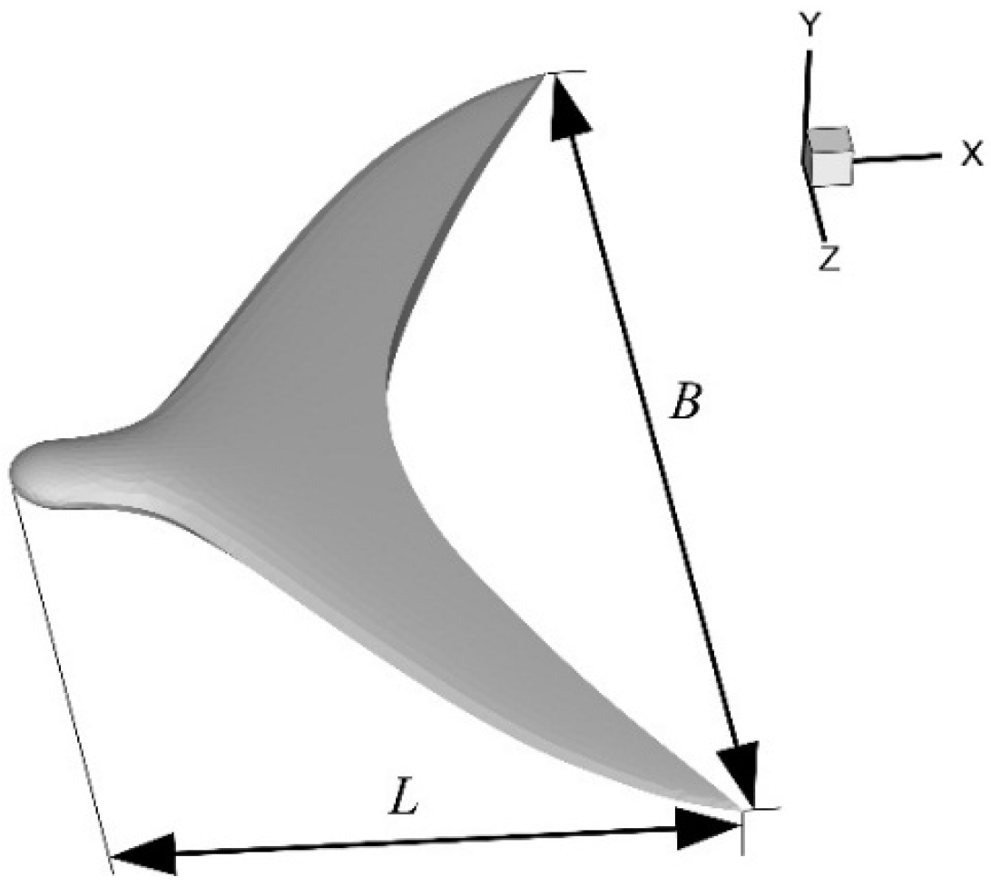
2.1. The Geometric Model of a Caudal Fin

The fins or wings of animals in nature have streamlined sections parallel to the flow direction. In this paper, the geometric model of caudal fin is accomplished with the curve-fitting method. In order to reduce the unwanted influence of leading edge, an elliptical structure is adopted. The three-dimensional geometry model is shown in Figure 1. The chord length L is 0.15 m, the length along the span direction B is 0.333 m, and the projected area (one-sided) S is 1.469 × 10⁻² m².

Figure 1. Geometric model of the fin.

Figure 1. Geometric model of the fin.

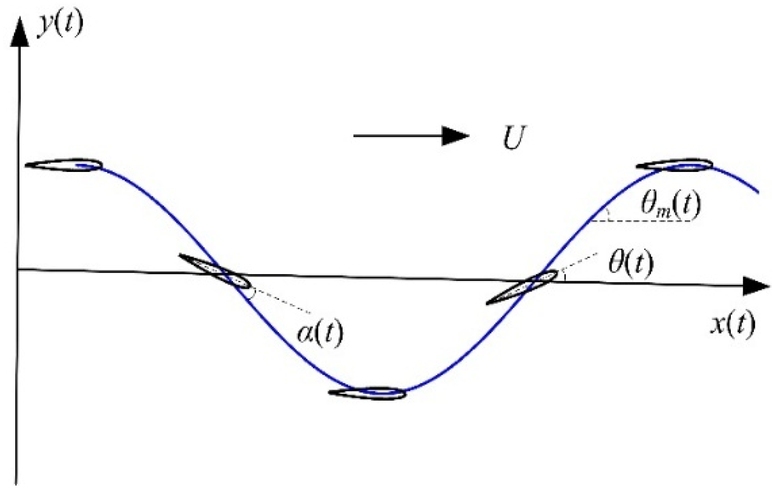
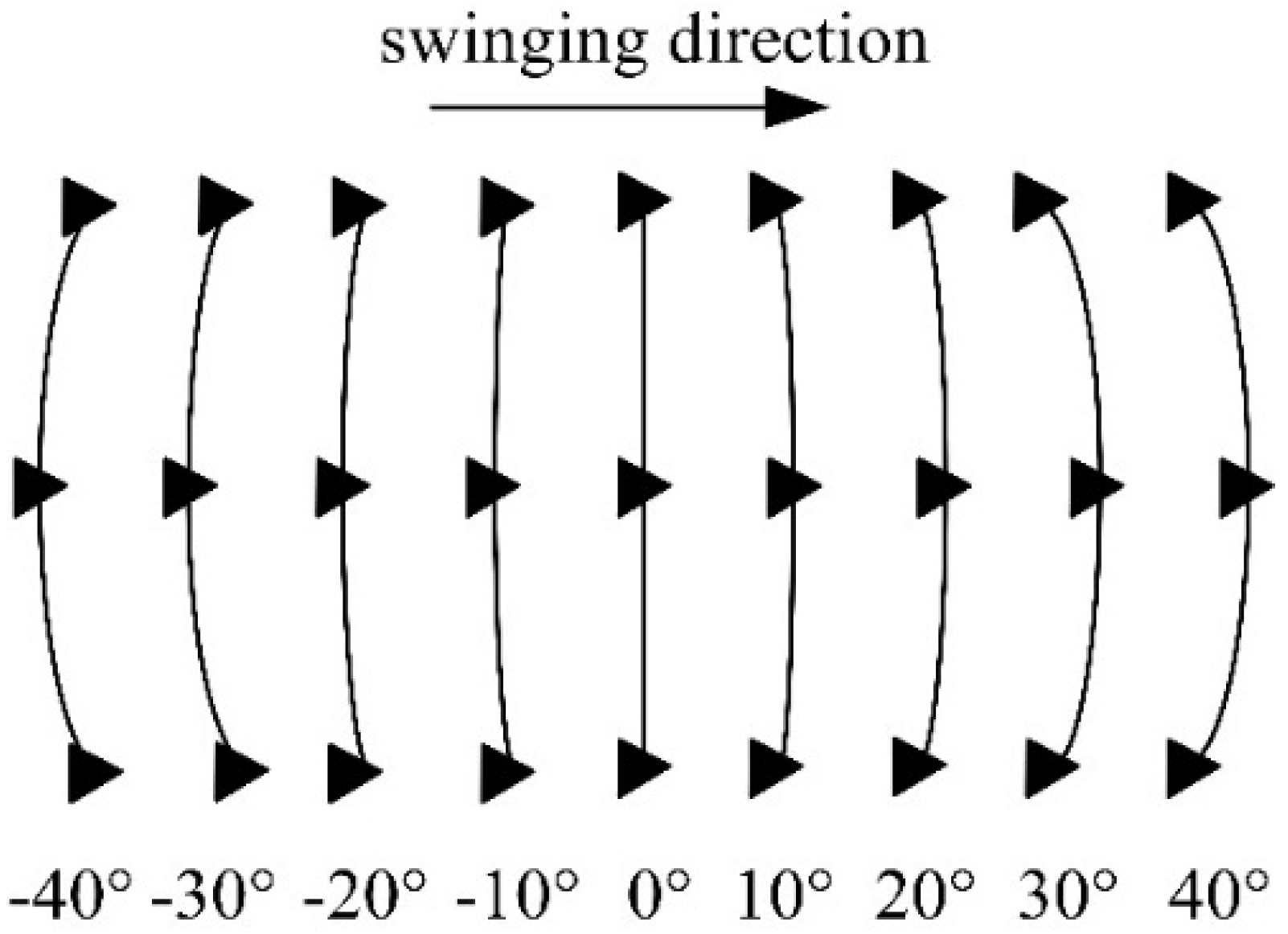
2.2. The Motion Model of Caudal Fin

The self-propulsion model has the difficulties in conducting corresponding experimental investigation. Most of the experimental research usually gives the incoming flow velocity or the towing velocity of fin. In other words, the motion of the fin is imposed. Here, we adopt the imposed motion model. The fin is towed forward at constant speed U and is allowed to move in two degrees of freedom:

(a)

motion transversely to the direction of towing, or heave y(t); and

(b)

angular motion about a spanwise axis, or pitch θ(t).

The heave motion of the fin can be described by the equation:

$$y(t)=h\cos (2\mathsf{\pi }ft)$$

(1)

where f is the flapping frequency, t is the time, and h is amplitude of the heave motion. In addition, the pitching angle θ is given by:

$$\mathsf{\theta }(t)=\mathsf{\alpha }(t)+{\mathsf{\theta }}_m(t)$$

(2)

where

$${\mathsf{\theta }}_m(t)=\arctan \left(\frac{\dot{y}(t)}{U}\right)$$

(3)

The angle α(t) is the angle of attack and given by:

$$\mathsf{\alpha }(t)={\mathsf{\alpha }}_{max}\sin (2\mathsf{\pi }ft)$$

(4)

where α_max is amplitude of the angle of attack. It can be seen that the angle of fin motion θ_m is dependent on the velocity of the fin in the global reference frame. The definitions of the different angles are shown in Figure 2.

Figure 2. Definition of variables.

Figure 2. Definition of variables.

The chord Reynolds number and the Strouhal number St is defined by:

$$Re=\frac{UL}{\nu }$$

(5)

$$St=\frac{2fh}{U}$$

(6)

where ν is the fluid kinematic viscosity. As is shown in [8], the forces and torque are converted to dimensionless forms and should be described by:

$$C_x(t)=\frac{F_x(t)}{0.5\rho U^{2}S}$$

(7)

$$C_y(t)=\frac{F_y(t)}{0.5\rho U^{2}S}$$

(8)

$$C_m(t)=\frac{M_{\mathsf{\theta }}(t)}{0.5\rho U^{2}SL}$$

(9)

Here, ρ is the density of the fluid, F_y is the transverse force, F_x is the thrust force, M_θ is the torque, and S is the projected area of the fin (one-sided). As is shown in [8], the propulsive efficiency η is defined as the ratio of output power P_o to input power P_e which can be written as:

$$P_o(t)=\frac{1}{T}{\displaystyle {\int }_0^T{F}_x(t)Udt}$$

(10)

$$P_e(t)=\frac{1}{T}{\displaystyle {\int }_0^T\left[F_y(t)\dot{y}(t)+M_z(t)\dot{\mathsf{\theta }}(t)\right]dt}$$

(11)

$$\mathsf{\eta }=\frac{P_o}{P_e}$$

(12)

where T is the period of the motion of the fin.

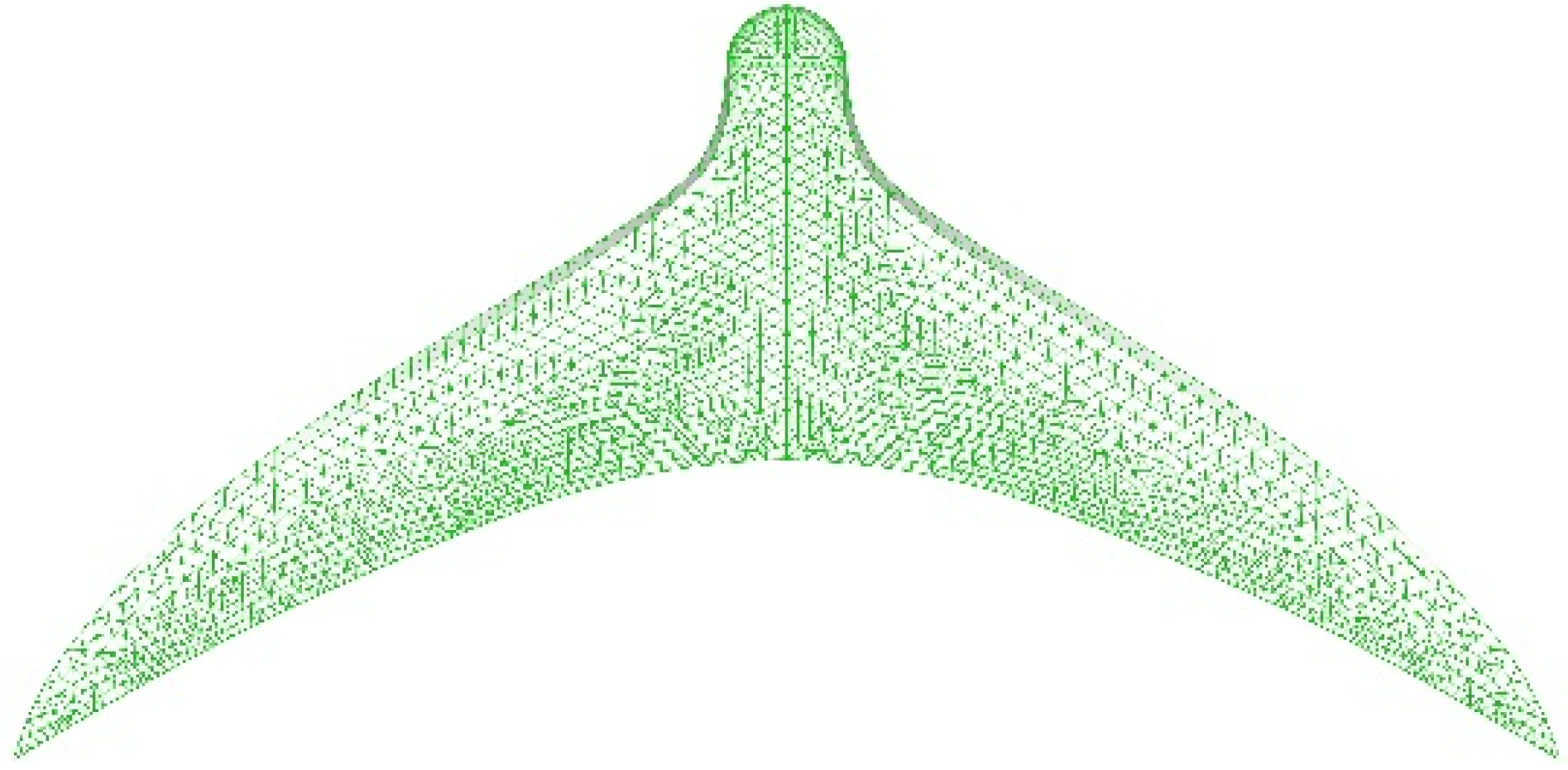
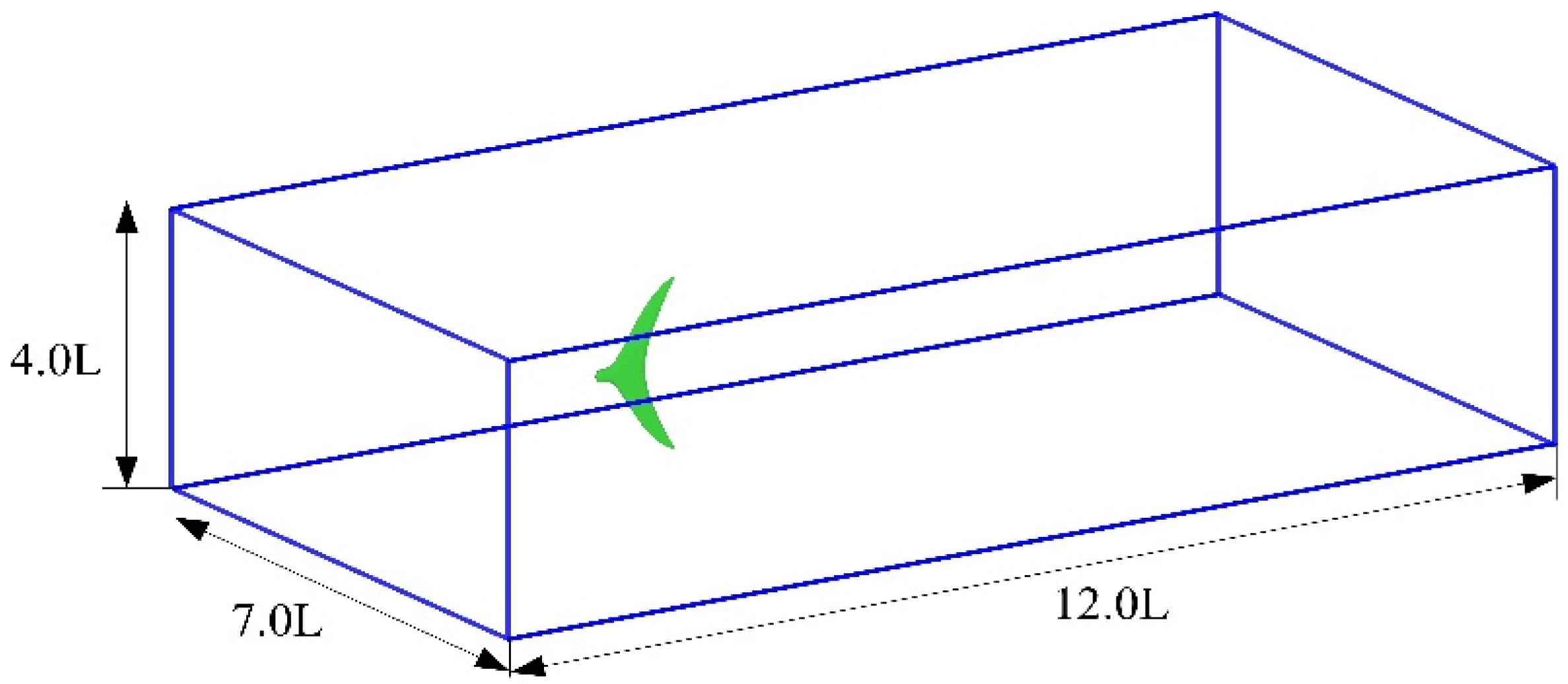
2.3. The Numerical Method

The Navier-Stokes equations for viscous and incompressible flows can be described by the equations:

$$\rho \left(\frac{\partial \mathit{u}}{\partial t}+\mathit{u}\cdot \nabla \mathit{u}\right)=-\nabla p+\mathsf{\mu }{\nabla }^2\mathit{u}$$

(13)

$$\nabla \cdot \mathit{u}=0$$

(14)

where u is the fluid velocity, ρ is the density, p is the pressure, and μ is the dynamic viscosity. Using the commercial software Fluent (ANSYS Inc., Canonsburg, PA, USA), the governing equations are discretized by the Finite Volume Method (FVM) with first-order discretization in time and second-order in space. The fluid field is computed on an unstructured, tetrahedral mesh. In order to improve calculation efficiency, a fine mesh is used near the moving surface and coarse mesh is used far away from the moving surface. The surface of the moving fin consists of triangle elements. The grids of the caudal fin are shown in Figure 3. The fluid field is divided into 8.9 × 10⁵ elements. To test the grid independency, the calculation with smaller cell size is carried out, but little difference between the coarse grid and the fine grid is found. The impact from the caudal fin to the fluid is carried out by imposing wall boundary conditions on the moving surface. The boundary conditions of the overall computation domain are set as symmetry boundary condition.

In the numerical simulations, the caudal fin starts to move from rest. Due to the movements of the fin, the grids around the moving surface need to be updated. Using the Fluent software, a dynamic mesh is applied to solve the problem. Furthermore, layering and local remeshing methods are used in the dynamic mesh to guarantee the stability of the calculation. The mesh is set to be updated in each time step. In the paper, the motion of the moving surface is specified in user-defined functions (UDF) linked to Fluent in the dynamical simulation. As is described by the motion equations, the caudal fin is towed forward at constant speed U and is set to carry out the heave motion and pitch motion. Without taking into account the flexibility, the caudal fin can be treated as a rigid body. In the paper, the DEFINE_CG_MOTION function is adopted to simulate the motion of the rigid fin. Using the DEFINE_CG_MOTION function, the translational and rotational motion of the rigid body can be defined in each time step. Taking into account the flexibility, the caudal fin can not be treated as a rigid body. Here the DEFINE_GRID_MOTION function is adopted to simulate the motion of the flexible fin. Using the DEFINE_GRID_MOTION function, the deformation velocity of each grid point can be defined in each time step. The deformation velocity of each grid point can be calculated through motion equations. Each motion period is divided into 200 time steps and the maximum number of iteration step in a time step is set to 50. In addition, the SIMPLE method is adopted to solve the pressure-velocity coupling problem. After several motion periods, the performance curves settle to a periodic behaviour. The calculation procedure takes 6–8 h per cycle on the personal computer. In order to eliminate the influences of the walls, enough space is kept around the caudal fin. The size of computational domain is shown in Figure 4.

Figure 3. Grids of caudal fin.

Figure 3. Grids of caudal fin.

Figure 4. Schematic of computational domain.

Figure 4. Schematic of computational domain.

Based on the existing experimental results [8], numerical simulations of flapping foil are conducted to verify the accuracy of the basic algorithm. The motion parameters of the foil are selected as follows: Re = 11000, St = 0.3, h = L = 0.055 m, B = 0.3575 m, and α_max = 25°.

Figure 5. Performance curves of flapping foil.

Figure 5. Performance curves of flapping foil.

Figure 5 shows the time histories of the force coefficients and torque coefficient of the fin. It is shown that the force coefficients and torque coefficient settle to a periodic behavior. There are two peaks in a period which are caused by the motions of downstroke and upstroke, respectively. Furthermore, the mean C_x is 0.58, the mean C_y is 0.0065, and the thrust efficiency is about 47.0%. Figure 6 shows the vortex pattern in the wake. It can be seen that the vortex rings exist in the wake. Vortex structures are depicted by the Q criterion [15,25]. Through the comparison, it is found that the present results compare well with those in experimental researches. Table 1 shows the reference results and present results.

Figure 6. Vortex pattern behind the foil.

Figure 6. Vortex pattern behind the foil.

Table 1. Reference results of flapping foil.

Case	Mean Cx	Mean Cy	Thrust Efficiency
Reference	0.604	0.0082	49.1%
Present	0.58	0.0065	47.0%

Table 1. Reference results of flapping foil.

Case	Mean Cx	Mean Cy	Thrust Efficiency
Reference	0.604	0.0082	49.1%
Present	0.58	0.0065	47.0%

3. Results and Discussion

The motion parameters of the caudal fin are selected as follows: Re = 45000, St = 0.3, h = 0.4 L, and α_max = 25°. For flapping foil propulsion, high-efficiency thrust production occurs in wakes with a Strouhal number in the range of 0.2 < St < 0.4 [8]. Furthermore, most fishes have been shown to swim near a “universal” optimal value St = 0.3 because of the high propulsive efficiency [29,30,31]. Therefore, St adopted in the paper is 0.3. Figure 7 shows the performance curves of caudal fin. It is shown that the curve settle to a similar behaviour with the flapping foil. It is further noticed that, the mean C_x which equals to 0.44 is positive and the mean C_y which equals to 0.002 is almost zero. In other words, the fin gets the thrust force and the resultant force of transverse force is near zero. The thrust efficiency is about 30.3%.

Figure 7. Performance curves of caudal fin.

Figure 7. Performance curves of caudal fin.

Figure 8 shows the vortex pattern in the wake. The vortex ring consists of a train of inverted hairpin-like vortices braided together such that the legs of each vortex are attached to the head of the preceding vortex [32,33]. Specifically, Figure 9 shows the two-dimensional vorticity magnitude in the wake. It is shown that the vortices shedding from the fin range two ranks and the vortices have different directions of rotation in different ranks. The jet stream can be induced between the two vortices ranks and the fin can obtain reaction force correspondingly. Furthermore, two vortices shed from the fin in a cycle time, resulting in two oscillations of thrust force.

Figure 8. Vortex pattern behind the fin.

Figure 8. Vortex pattern behind the fin.

Figure 9. Two-dimensional vorticity contours in the wake.

Figure 9. Two-dimensional vorticity contours in the wake.

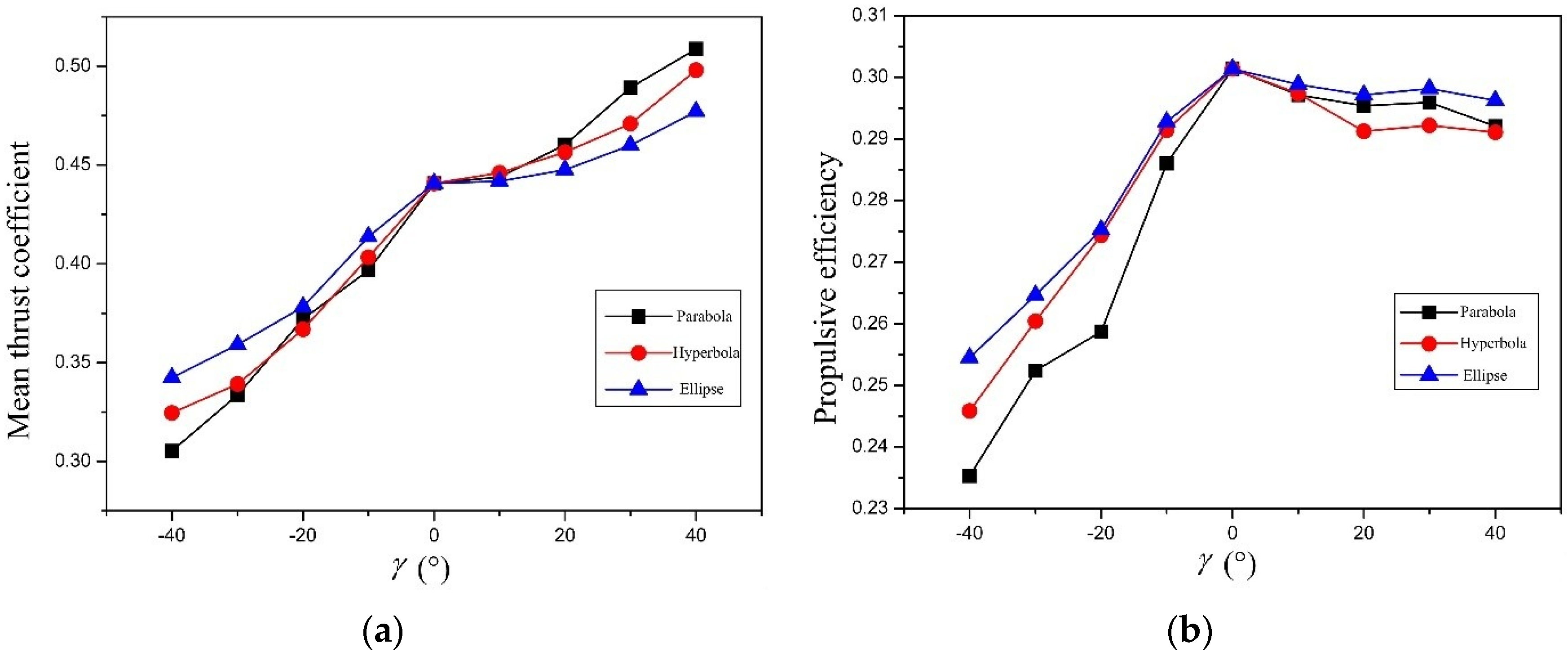
3.1. Influence of the Amplitude of Angle of Attack

Figure 10 shows the performance curves versus versus amplitude of angle of attack. As the angle of attack increases, the mean thrust force increases correspondingly and reaches the peak point, then starts to decreases. The mean thrust force keeps a relatively large value when the angle of attack α_max varies from 20° to 30°, which is consistent with tuna in nature. Additionall, it is found that the propulsive efficiency has similar trend compared with mean thrust force. The propulsive efficiency achieves peak point between α_max = 20° and α_max = 30°. With larger or smaller α_max, it will impart a large transverse force and reduce thrust force, and then decrease the propulsive efficiency. Figure 11 shows the vortex pattern in the wake at different α_max. The volume of the vortex blob is smaller at α_max = 25°, which results in lower energy dissipation in the wake.

Figure 10. Performance curves: mean thrust coefficient versus versus angle of attack: (a) mean thrust coefficient; (b) propulsive efficiency.

Figure 10. Performance curves: mean thrust coefficient versus versus angle of attack: (a) mean thrust coefficient; (b) propulsive efficiency.

Figure 11. Vortex pattern in the wake: (a) α_max = 25°; (b) α_max = 10°.

Figure 11. Vortex pattern in the wake: (a) α_max = 25°; (b) α_max = 10°.

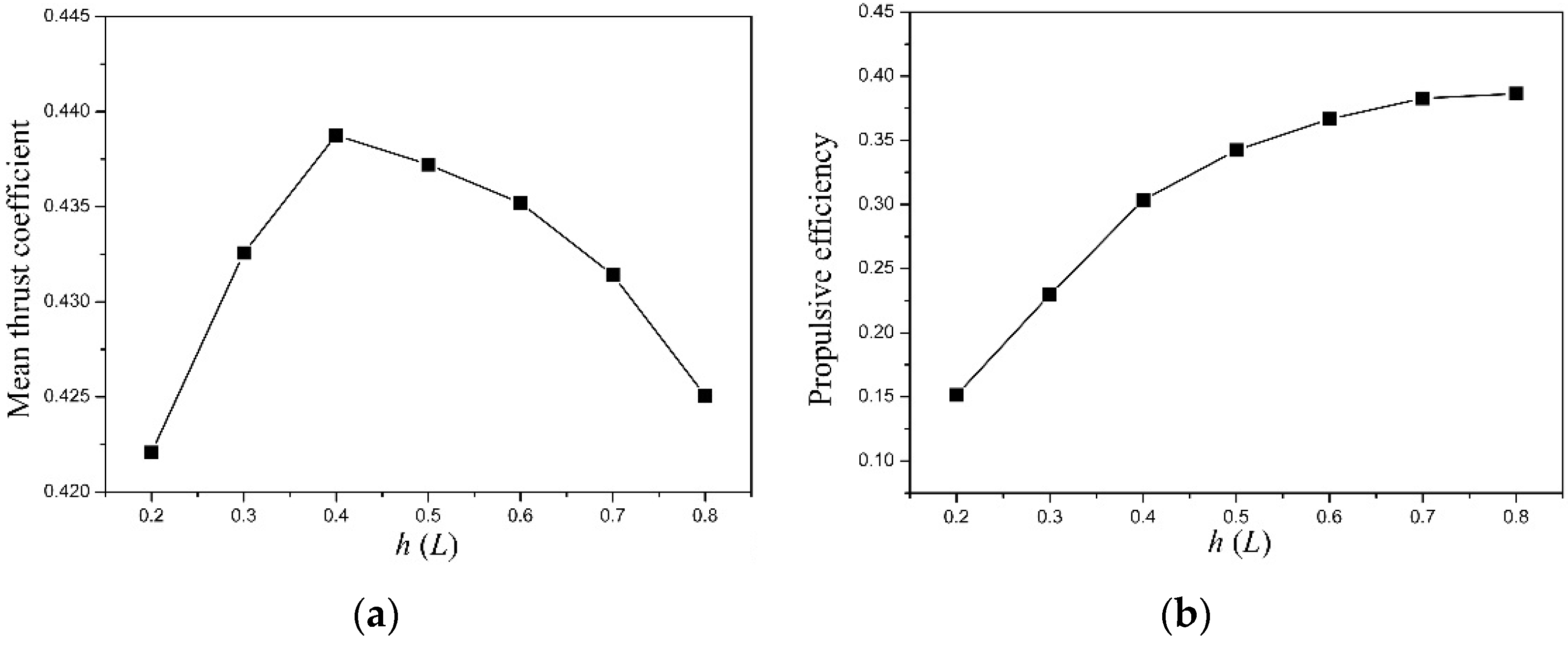
3.2. Influence of the Amplitude of Heave Motion

To investigate the influence of heave motion, the amplitude of heave motion h is chosen to vary from 0.2 L to 0.8 L and the Strouhal number remains constant. Figure 12 shows the performance curves of caudal fin. The mean thrust force achieves the maximum at h = 0.4 L but the effect of amplitude of heave motion is insignificant. As is known to all, large heave motion will obviously lead to a large thrust force, but a larger heave motion will lead to a lower frequency to keep the Strouhal number constant. Thus, the change of mean thrust is insignificant when the amplitude of the heave motion h increases. In nature, the amplitude of caudal fin usually keeps 0.3–0.5 L. In this case, fish with caudal fin propulsion can achieve high propulsive efficiency correspondingly with larger thrust force. As is shown in Figure 13, the vortex structure is more compact because of higher frequency, which enlarges the energy consumption.

Figure 12. Performance curves versus amplitude of heave motion: (a) mean thrust coefficient; (b) propulsive efficiency.

Figure 12. Performance curves versus amplitude of heave motion: (a) mean thrust coefficient; (b) propulsive efficiency.

Figure 13. Vortex pattern in the wake: (a) h = 0.4 L; (b) h = 0.2 L.

Figure 13. Vortex pattern in the wake: (a) h = 0.4 L; (b) h = 0.2 L.

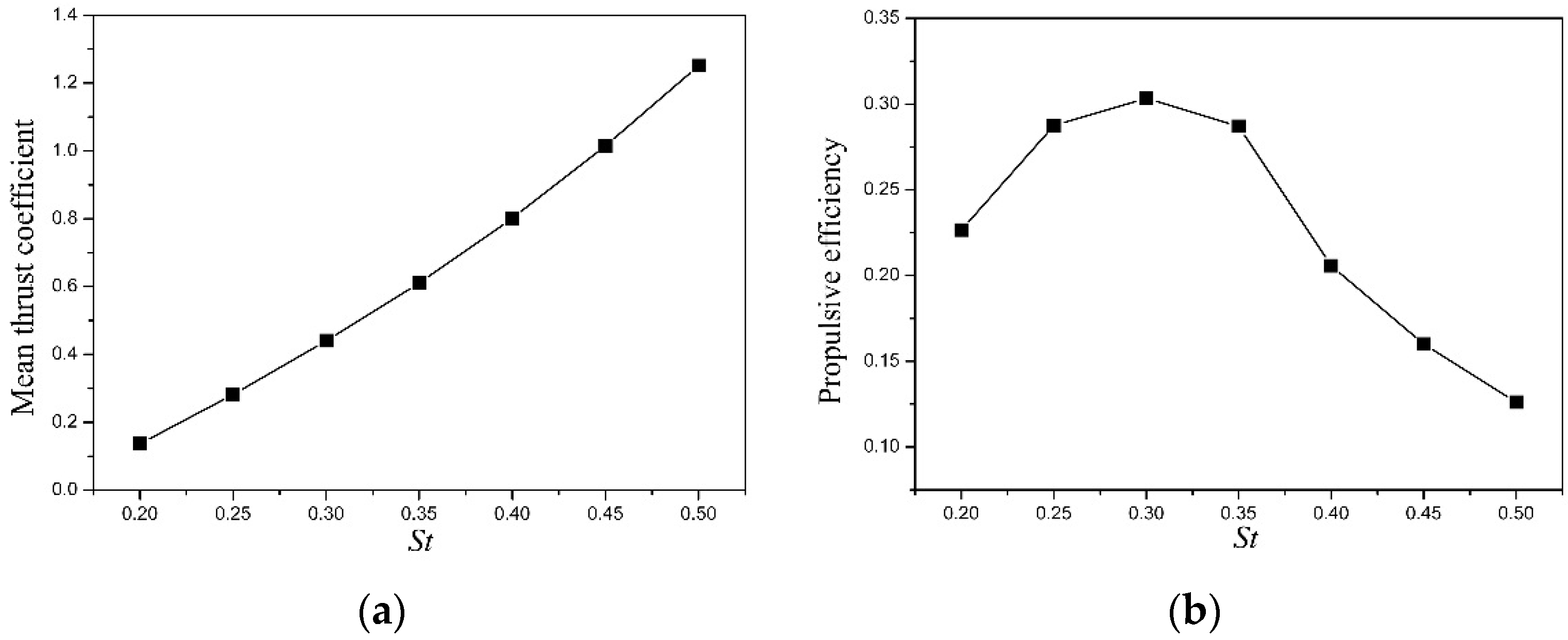
3.3. Influence of the Amplitude of Strouhal Number

Strouhal number, St, is an important parameter in the biological swimming. Here, a different Strouhal number is adopted in the numerical simulations by choosing a different flapping frequency varying from 0.5 Hz to 2.0 Hz. Figure 14 shows the performance curves versus the Strouhal number. It is found that the mean thrust force increases approximately linearly when the Strouhal number increases. During the startup or accelerating stage, fish also rapidly oscillate to get large thrust force and advancing speed. The propulsive efficiency keeps a large value when the Strouhal number is 0.25–0.40. This is consistent with fish in nature. Figure 15 shows the vortex pattern in the wake at different St. At low St, the 3D structure of the wake is shown a single and continuous vortex ring. At higher St, a more complex and laterally-diverging structure is observed in the wake. Smaller-scale vertical structures attaching to the hairpin vortices are observed in the wake. The pattern consists of complex and highly 3D coherent structures and the vortex structure is more compact. The energy dissipation is greater in this case, so the propulsive efficiency is lower at high St.

Figure 14. Performance curves versus Strouhal number: (a) mean thrust coefficient; (b) propulsive efficiency.

Figure 14. Performance curves versus Strouhal number: (a) mean thrust coefficient; (b) propulsive efficiency.

Figure 15. Vortex pattern in the wake: (a) St = 0.3; (b) St = 0.5.

Figure 15. Vortex pattern in the wake: (a) St = 0.3; (b) St = 0.5.

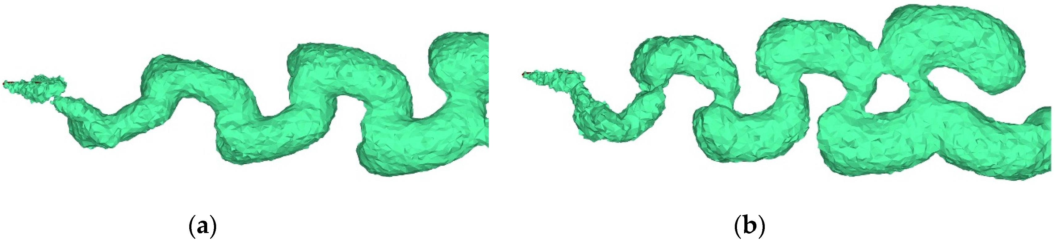
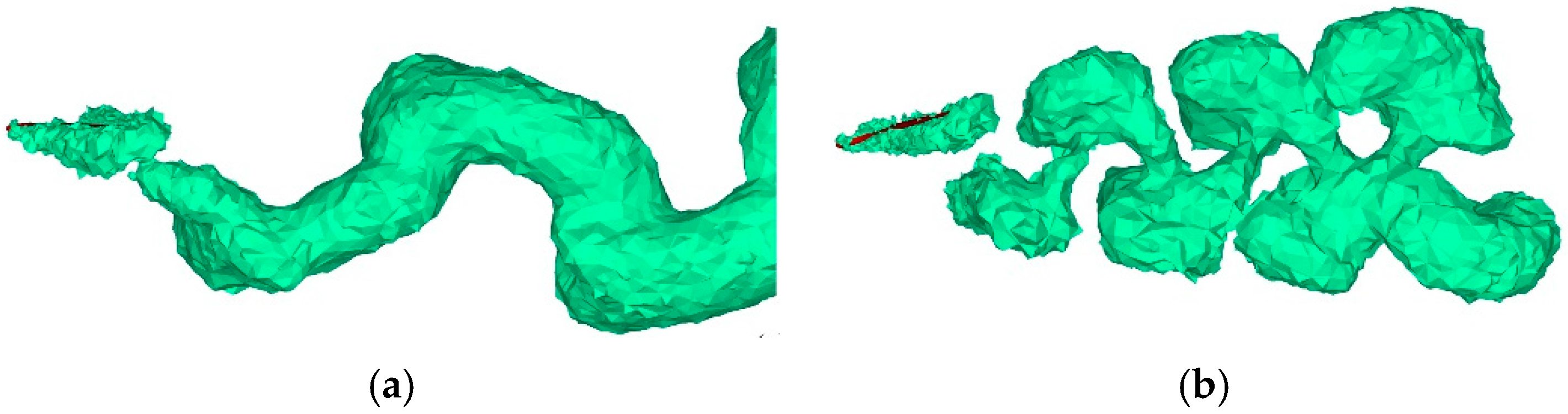
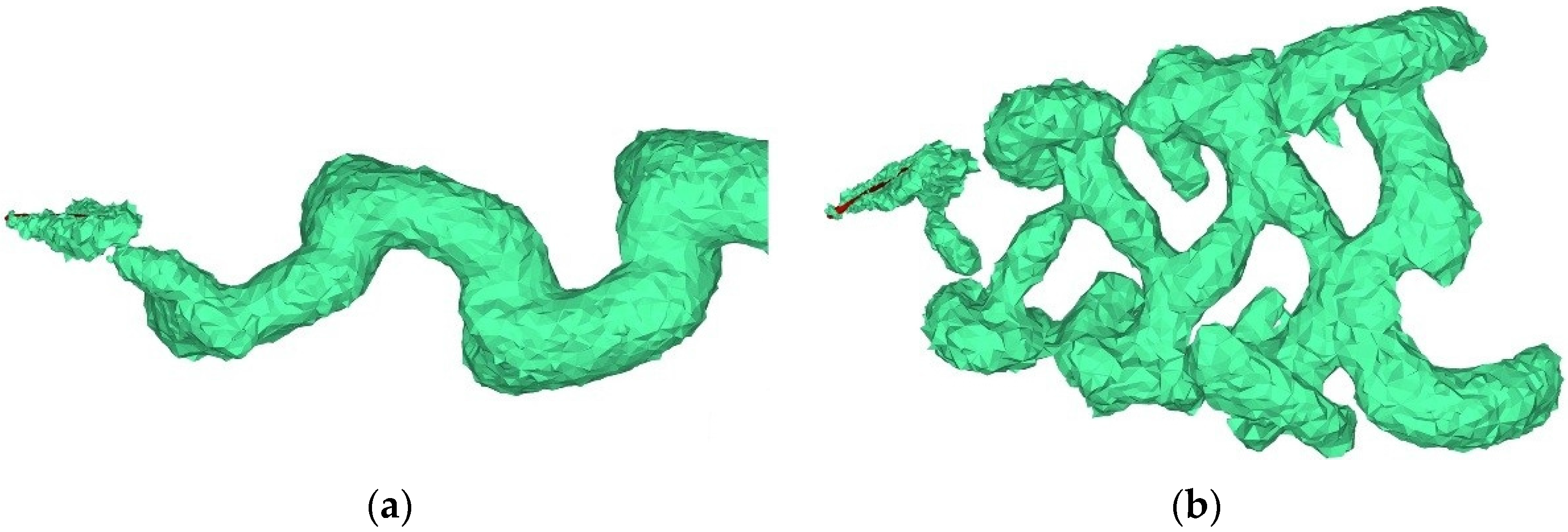
3.4. Influence of the Spanwise Flexibility

In nature, caudal fin is usually flexible and the flexibility plays an important role in the motion of fish. So the flexibility should be considered in the modeling of caudal fin. However, the flexibility problem is complicated and the modeling of the problem is very difficult. In addition, the flexibility in nature is not controllable. Thus, the paper applies an imposed motion to the original motion model. In this way the influences of flexibility can be investigated more intuitively and the flexibility motion model can also easily adopted in engineering applications. Therefore, the spanwise flexibility is introduced in the model. Here, the phase angle γ is adopted to describe spanwise flexibility. At certain chordwise positions, the phase angle γ describes the phase difference of pitch motion between edge point and center point of the caudal fin. Here, the angle of attack α(t) of the edge points can be written as:

$$\mathsf{\alpha }(t)={\mathsf{\alpha }}_{max}\sin (2\mathsf{\pi }ft-\mathsf{\gamma })$$

(15)

At any time, the coordinates of edge point and center point can be obtained. Using different curve functions, these three points can determine a curve and the coordinates of any point along the spanwise direction can be calculated through curve functions. Figure 16 shows the shape of fin along the spanwise direction with different phase angle γ.

Figure 16. Schematic of spanwise flexibility and γ value.

Figure 16. Schematic of spanwise flexibility and γ value.

The performance curves versus phase angle are shown in Figure 17. In this paper, elliptic curve, hyperbolic curve, and parabolic curve are adopted in simulations. It can be seen that the case with the elliptic curve can achieve higher propulsive efficiency. Furthermore, the fin can get larger thrust force with high propulsive efficiency when the phase angle keeps a positive value, which is consistent with fish in nature.

Figure 17. Performance curves versus phase angle: (a) mean thrust coefficient; (b) propulsive efficiency.

Figure 17. Performance curves versus phase angle: (a) mean thrust coefficient; (b) propulsive efficiency.

4. Conclusions

In this paper, numerical simulations of caudal fin propulsion are conducted. To verify the accuracy of the basic algorithm, numerical simulations of the flapping foil are conducted. The present results compare well with those in experimental research. Thus, the algorithm adopted in the paper is reliable. After that, influences of the amplitude of angle of attack, the amplitude of heave motion, the Strouhal number, and the spanwise flexibility are analyzed. The results show that the caudal fin can get thrust force due to the self motion and vortex rings exist in the wake. Additionally, the performance can be improved by adjusting the motion parameters. Furthermore, the fin can get larger thrust force with high propulsive efficiency when the phase angle keeps a positive value. The results of this paper would provide theoretic reference for the design of an underwater vehicle based on flapping propulsion.

The paper attempts to analyze the mechanism and factors affecting the performance of caudal fin propulsion. However, fish locomotion is certainly far more complex and diverse than the simple model considered here. Furthermore, corresponding experimental research should be conducted. This work will be conducted in the future.

References

1. Yan, Y.Y. Recent advances in computational simulation of macro-, meso-, and micro-scale biomimetics related fluid flow problems. J. Bionic Eng. 2007, 4, 97–107. [Google Scholar] [CrossRef]
2. Mittal, R. Computational modeling in biohydrodynamics: Trends, challenges, and recent advances. IEEE J. Ocean. Eng. 2004, 29, 595–604. [Google Scholar] [CrossRef]
3. Tian, F.B.; Luo, H.X.; Zhu, L.D.; Liao, J.C.; Lu, X.Y. An efficient immersed boundary-lattice Boltzmann method for the hydrodynamic interaction of elastic filaments. J. Comput. Phys. 2011, 230, 7266–7283. [Google Scholar] [CrossRef] [PubMed]
4. Tian, F.B.; Lu, X.Y.; Luo, H.X. Propulsive performance of a body with a traveling-wave surface. Phys. Rev. E 2012, 86. [Google Scholar] [CrossRef] [PubMed]
5. Ramananarivo, S.; Godoy-Diana, R.; Thiria, B. Rather than resonance, flapping wing flyers may play on aerodynamics to improve performance. Proc. Natl. Acad. Sci. USA 2011, 108, 5964–5969. [Google Scholar] [CrossRef] [PubMed]
6. Unger, R.; Haupt, M.C.; Horst, P.; Radespiel, R. Fluid-structure analysis of a flexible flapping airfoil at low Reynolds number flow. J. Fluids Struct. 2012, 28, 72–88. [Google Scholar] [CrossRef]
7. Wang, S.Z.; Zhang, X.; He, G.W. Numerical simulation of a three-dimensional fish-like body swimming with finlets. Commun. Comput. Phys. 2012, 11, 1323–1333. [Google Scholar] [CrossRef]
8. Izraelevitz, J.S.; Triantafyllou, M.S. Adding in-line motion and model-based optimization offers exceptional force control authority in flapping foils. J. Fluid Mech. 2014, 742, 5–34. [Google Scholar] [CrossRef]
9. Szymik, B.G.; Satterlie, R.A. Changes in wingstroke kinematics associated with a change in swimming speed in a pteropod mollusk, Clione limacina. J. Exp. Biol. 2011, 214, 3935–3947. [Google Scholar] [CrossRef] [PubMed]
10. Triantafyllou, M.S.; Techet, A.H.; Hover, F.S. Review of experimental work in biomimetic foils. IEEE J. Ocean. Eng. 2004, 29, 585–594. [Google Scholar] [CrossRef]
11. Deng, H.B.; Xu, Y.Q.; Chen, D.D.; Dai, H.; Wu, J.; Tian, F.B. On numerical modeling of animal swimming and flight. Comput. Mech. 2013, 52, 1221–1242. [Google Scholar] [CrossRef]
12. Luo, H.X.; Mittal, R.; Zheng, X.D.; Bielamowicz, S.A.; Walsh, R.J.; Hahn, J.K. An immersed-boundary method for flow—Structure interaction in biological systems with application to phonation. J. Comput. Phys. 2008, 227, 9303–9332. [Google Scholar] [CrossRef] [PubMed]
13. Zhang, X.; Schmidt, D.; Perot, B. Accuracy and conservation properties of a three-dimensional unstructured staggered mesh scheme for fluid dynamics. J. Comput. Phys. 2002, 175, 764–791. [Google Scholar] [CrossRef]
14. Zhang, X.; Ni, S.Z.; He, G.W. A pressure-correction method and its applications on an unstructured Chimera grid. Comput. Fluids 2008, 37, 993–1010. [Google Scholar] [CrossRef]
15. Li, G.J.; Zhu, L.D.; Lu, X.Y. Numerical studies on locomotion performance of fish-like tail fins. J. Hydrodyn. 2012, 24, 488–495. [Google Scholar] [CrossRef]
16. Wu, J.; Shu, C. Simulation of three-dimensional flows over moving objects by an improved immersed boundary—Lattice Boltzmann method. Int. J. Numer. Methods Fluids 2012, 68, 977–1004. [Google Scholar] [CrossRef]
17. Atzberger, P.J.; Kramer, P.R.; Peskin, C.S. A stochastic immersed boundary method for fluid-structure dynamics at microscopic length scales. J. Comput. Phys. 2007, 224, 1255–1292. [Google Scholar] [CrossRef]
18. Zhu, L.D.; He, G.W.; Wang, S.Z.; Miller, L.; Zhang, X.; You, Q.; Fang, S. An immersed boundary method based on the lattice Boltzmann approach in three dimensions, with application. Comput. Math. Appl. 2011, 61, 3506–3518. [Google Scholar] [CrossRef]
19. Mittal, R.; Dong, H.; Bozkurttas, M.; Najjar, F.M.; Vargas, A.; von Loebbecke, A. A versatile sharp interface immersed boundary method for incompressible flows with complex boundaries. J. Comput. Phys. 2008, 227, 4825–4852. [Google Scholar] [CrossRef] [PubMed]
20. Liao, C.C.; Chang, Y.W.; Lin, C.A.; McDonough, J.M. Simulating flows with moving rigid boundary using immersed-boundary method. Comput. Fluids 2010, 39, 152–167. [Google Scholar] [CrossRef]
21. Lima E Silva, A.L.F.; Silveira-Neto, A.; Damasceno, J.J.R. Numerical simulation of two-dimensional flows over a circular cylinder using the immersed boundary method. J. Comput. Phys. 2003, 189, 351–370. [Google Scholar] [CrossRef]
22. Gilmanov, A.; Sotiropoulos, F. A hybrid Cartesian/immersed boundary method for simulating flows with 3D, geometrically complex, moving bodies. J. Comput. Phys. 2005, 207, 457–492. [Google Scholar] [CrossRef]
23. Ge, L.; Sotiropoulos, F. A numerical method for solving the 3D unsteady incompressible Navier-Stokes equations in curvilinear domains with complex immersed boundaries. J. Comput. Phys. 2007, 225, 1782–1809. [Google Scholar] [CrossRef] [PubMed]
24. Borazjani, I.; Sotiropoulos, F. On the role of form and kinematics on the hydrodynamics of self-propelled body/caudal fin swimming. J. Exp. Biol. 2010, 213, 89–107. [Google Scholar] [CrossRef] [PubMed]
25. Borazjani, I.; Sotiropoulos, F. Numerical investigation of the hydrodynamics of carangiform swimming in the transitional and inertial flow regimes. J. Exp. Biol. 2008, 211, 1541–1558. [Google Scholar] [CrossRef] [PubMed]
26. Dong, H.; Mittal, R.; Najjar, F.M. Wake topology and hydrodynamic performance of low-aspect-ratio flapping foils. J. Fluid Mech. 2006, 566, 309–343. [Google Scholar] [CrossRef]
27. Heathcote, S.; Wang, Z.; Gursul, I. Effect of spanwise flexibility on flapping wing propulsion. J. Fluids Struct. 2008, 24, 183–199. [Google Scholar] [CrossRef]
28. Zhu, Q.; Shoele, K. Propulsion performance of a skeleton-strengthened fin. J. Exp. Biol. 2008, 211, 2087–2100. [Google Scholar] [CrossRef] [PubMed]
29. Triantafyllou, M.S.; Triantafyllou, G.S.; Yue, D.K.P. Hydrodynamics of fishlike swimming. Annu. Rev. Fluid Mech. 2000, 32, 33–53. [Google Scholar] [CrossRef]
30. Taylor, G.K.; Nudds, R.L.; Thomas, A.L.R. Flying and swimming animals cruise at a Strouhal number tuned for high power efficiency. Nature 2003, 425, 707–711. [Google Scholar] [CrossRef] [PubMed]
31. Thomas, A.L.R.; Taylor, G.K.; Srygley, R.B.; Nudds, R.L.; Bomphrey, R.J. Dragonfly flight: Free-flight and tethered flow visualizations reveal a diverse array of unsteady lift-generating mechanisms, controlled primarily via angle of attack. J. Exp. Biol. 2004, 207, 4299–4323. [Google Scholar] [CrossRef] [PubMed]
32. Govardhan, R.N.; Williamson, C.H.K. Vortex-induced vibrations of a sphere. J. Fluid Mech. 2005, 531, 11–47. [Google Scholar] [CrossRef]
33. Buchholz, J.H.; Smits, A.J. On the evolution of the wake structure produced by a low-aspect-ratio pitching panel. J. Fluid Mech. 2006, 546, 433–443. [Google Scholar] [CrossRef] [PubMed]