1. Introduction
In recent years, the power grids have become more stressed due to growing consumer demand and less secure with the penetration of distributed generation resources. Moreover, the increasing share of fossil fuel usage during peak hours raises environmental concerns. Since more than one-third of the electrical energy is consumed at residential premises, one effective way to address the aforementioned challenges is the employment of smart home energy management systems. Such systems integrate communication, control and sensing technologies to efficiently shape the electricity consumption [
1]. Therefore, this paper proposes a new energy scheduling framework for a group of households having different numbers of occupants, family decompositions and employment statuses equipped with a variety of home appliances [
2]. The model aims to exploit the diversity in the customer preferences and shows that the cost of electricity consumption can be reduced by scheduling the jobs within a time window that is acceptable by the consumers.
There has been an increasing body of literature on demand response management programs [
3,
4]. Some examples include the lowering of peak customer demand [
5] by shifting the consumption towards the periods of high renewable energy production [
6]. However, this approach requires the jobs to be very flexible, because the time of the generation and the demand may not perfectly align. Overall, the vast majority of the optimization problems presented in the literature are closely related to different variations of classical optimization, such as job scheduling and load balancing [
7,
8,
9]. The scheduling is done based on the requests from the consumers, which are given in advance for individual appliances with flexible timeslots. For example, a consumer can request the use of a dishwasher during the time period between 12 and 2 p.m. or 5 and 7 p.m. Similarly, if the user has a plug-in electric vehicle, he or she would like the vehicle battery to be fully charged by 7 a.m. Based on the collected requests, the grid controller will schedule all such request with a specific duration in a way to optimize some performance parameters, such as minimizing the peak demand or the total cost of electricity production. It is noteworthy that this type of problem could also be considered in an online optimization in which consumer requests are given in real time [
10]. From this basic concept, many demand side models have been explored in varying levels of detail and system properties for electric vehicles [
11,
12,
13] and household appliances [
14,
15,
16,
17,
18,
19]. The objective function in such problems is, in most cases, based on the minimization of total electricity cost. The optimization frameworks also focus on cost-reductions during the peak hours, as the cost function typically follows a quadratic convex behavior, meaning that the increase in electric consumption over some level has disproportional increased the expenses needed to provide the service [
10,
14,
18].
In the paper by Salins
et al. [
20], the cost minimization problem is presented as a multi-objective one, which also takes the utilization levels into account. The computational complexity of the previously-developed models is proportional to the constraints used on the behavior of appliances, e.g., power levels and job deadlines. It has been shown that the offline scheduling problem with jobs (consumer request for individual appliances) having an arbitrary duration or an arbitrary power requirement is NP-complete [
10]. In the studies conducted by Burcea
et al. [
14], a simplified model is given, in which all of the home appliances have a unit power requirement, unit duration and arbitrary time slots for which the jobs can be served. For this problem, a polynomial time algorithm has been developed for finding optimal solutions. An extensive analysis of different appliances that can be a part of this problem is given in [
19].
Another critical point in the related scheduling problems is the relation between the “flexibility” of the loads and the associated electricity cost. The literature shows that when the time horizon for job scheduling is expanded, the customer demand can be met at a lower cost. The existing literature employs binary values to represent the operation of appliances at each time step, e.g., binary 1 shows that the appliance is “on” and consumes power, while binary 0 shows that the appliance is turned “off”. On the other hand, the behavior and the appliance usage habits in households of different sizes with varying occupants and ages can notably differ. For instance, young professionals may not prefer to do the laundry after midnight, whereas this can be a good money-saving option for pensioners. It is important to note that such habits are not dependent on the financial aspect cost [
2].
Similarly, one of the missing parts of the existing models is that the comfort levels are only limited to HVAC (heating, ventilating and air conditioning) appliances, and they are measured by the output temperature. Nevertheless, the idea of the “satisfaction-cost” trade-off has been neglected for other household devices. Here, we use the term “satisfaction” in the sense of using the appliance at times that are more or less convenient. The idea is that by adding such a property to job requests and by granting a minimal level of “satisfied preferences” to all of the consumers, the flexibility of time periods for jobs would increase; hence, the scheduling problem can be solved at a lower cost.
In this paper, we propose a model for the underlying scheduling problem that takes the preference/satisfaction levels into account. To be exact, we define a multi-objective optimization problem and analyze the relation between the two objectives by exploring the Pareto front on problem instances based on real-world household usage data from [
21] with real-world electricity prices. The paper is organized as follows. In
Section 2, we present the model and the corresponding mixed integer program. In
Section 3, we give the details of how real-world data are incorporated into the model. The results of the conducted computational experiments are presented in
Section 4.
3. Use of Real-World Data
For the proposed model, our goal is to explore its potential for real-world application; because of this, we generate test instances based on the measured data. More precisely, the consumer behavior and preferences are based on the data collected in a survey conducted by the Department of Energy & Climate Change, UK [
21]. The survey data were collected from 251 households in England over the period from May 2010–July 2011. For each of the households, the electrical power demand and energy consumption were monitored. The participating households were selected on the basis of the life-stage of the occupants. During the course of the survey period, the occupants also completed diaries of use for some of the products they used. They were also requested to complete survey questions about their environmental attitudes. There were no special incentives to influence the behavior of participants.
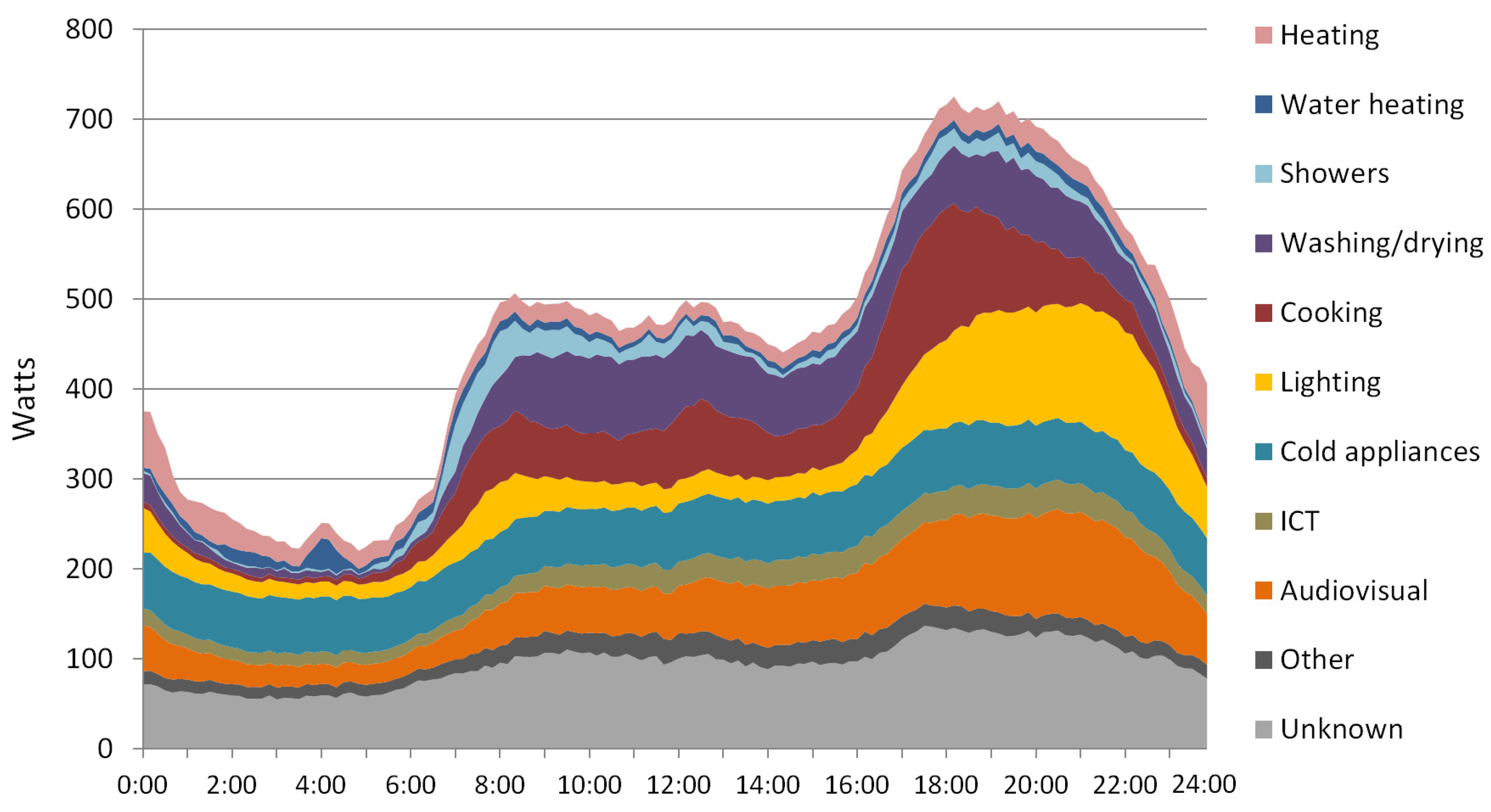
The households were divided into five groups: family with (FWC) and without children (FNC), multiple pensioners (MP), single pensioner (SP) and single non-pensioned (SNP). For each household and individual appliance, energy consumption has been monitored every 10 min. An illustration of aggregated data can bee seen in
Figure 2.
It is well known that some appliances, like lighting, audio/visual, computers,
etc., cannot be controlled without a significant impact on consumer comfort. Because of this fact, in the generated problem instances, we assume that only cooking and washing appliances could be scheduled. The energy consumption of the other appliances is used as a base load. It is important to point out that water heating appliances are also excluded from scheduling because the vast majority of surveyed households used natural gas instead of electricity (see
Figure 2). Although the monitored data show the energy consumption, they also give information on the time periods when households have used such appliances. To be more precise, a high level of energy consumption corresponded to a high number of working appliances at some time.
Figure 2.
Illustration of the hourly energy consumption of different appliances (per household) from survey data. The image corresponds to average energy consumption of all participating household for working days.
Figure 2.
Illustration of the hourly energy consumption of different appliances (per household) from survey data. The image corresponds to average energy consumption of all participating household for working days.
In the generation of problem instances, the energy consumption for each group of households is treated separately. It is understandable that there could be a high demand to use appliances of Type A at some time period
t, which indicates that many household have a preference for using
at
t. This simple logic is used to generate preferences (variables
) in the following way. The first step is to convert the hourly energy consumption curve
, for appliance type
and household type
, into a probability distribution. This can be done using the following formula:
In
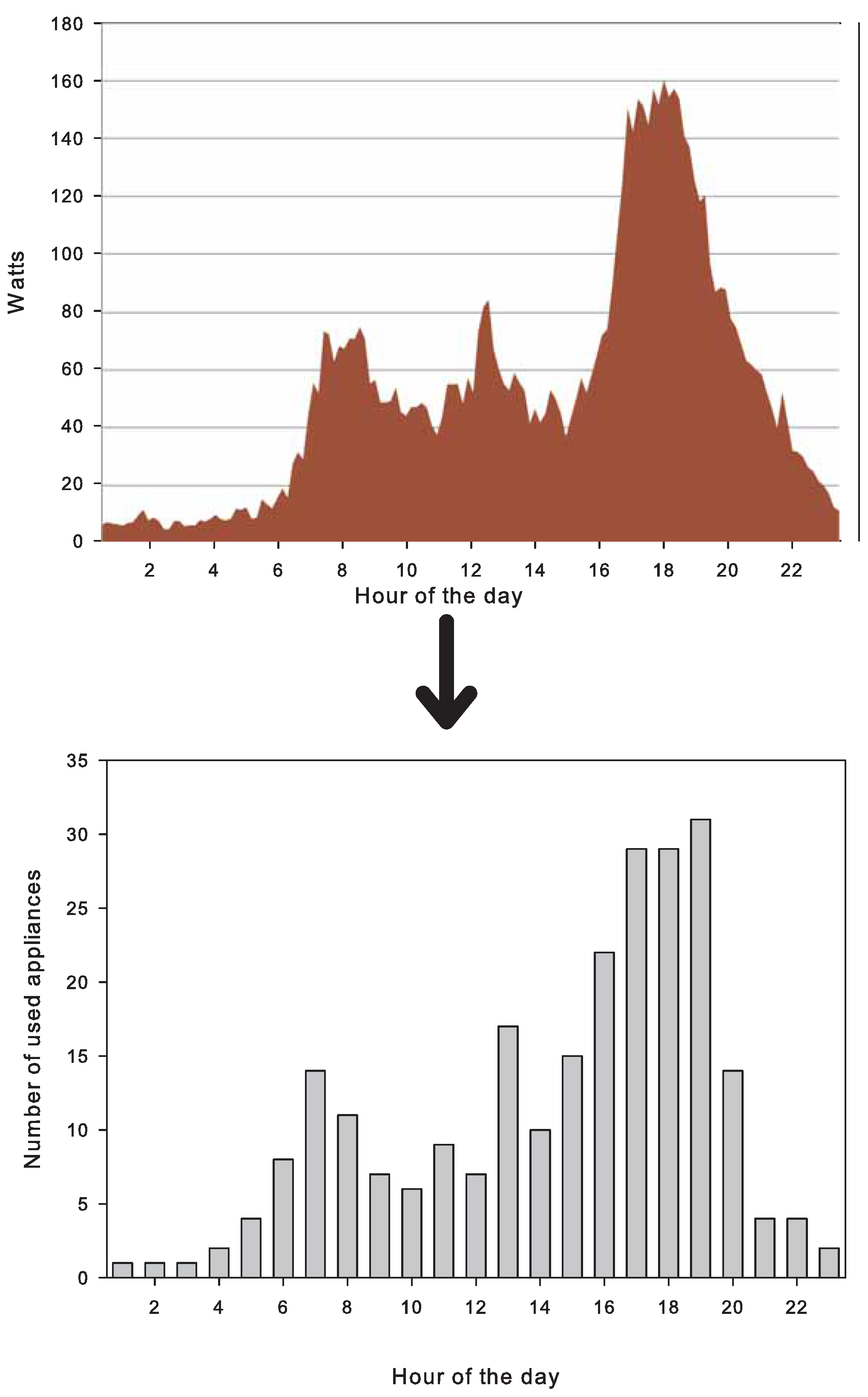
Figure 3, we show the distribution of oven working periods for 250 FWC using the corresponding probability distribution.
The procedure for generating preference levels for a specific household h and appliance a is done in the following way. Let us say that h is of type and a is of type . For simplicity, let us assume that operating time . Initially, all of the values of . Using the probability distribution , we would, one by one, select time periods for which the preference values would be set from 1–6. This is done iteratively, in an ascending order of i, by selecting a time period based on the probability distribution and setting , with the constraint . The procedure in case of is the same, except that the constraints forbid the overlapping of selected time intervals.
Figure 3.
Illustration of converting the average energy consumption of cooking appliances (per household) to the appliance use distribution.
Figure 3.
Illustration of converting the average energy consumption of cooking appliances (per household) to the appliance use distribution.
In our model, we take the operating times and the energy consumption of appliances from data provided by [
23,
24], and the values can be seen in
Table 1. For simplicity, in the model, we only use a single appliance for washing and drying machines having energy consumption equal to their average.
Table 1.
Energy use and operating time for different appliances.
Table 1.
Energy use and operating time for different appliances.
| Type | Time | kW |
|---|
| Stove | 1 | |
| Oven | 1 | |
| Washer dryer | 2 | |
| Dishwasher | 1 | |
The generated problem instances represent a time period of 24 h. One time period is equal to one full hour. At each time instance, the number of households
N and the number of them in each group (FWC, FWN, MP, SP and NSP) is proportional to the same values in the monitored data. These values are given in
Table 2. Furthermore, the probability of an individual household submitting a request for using an appliance is proportional to the frequency of appliance utilization. Approximate operating frequencies, for each group, in the case of washer/dryers and dishwashers could be derived from the survey data. In the case of cooking appliances, no precise data are given. For them, these values are specified based on experience. Further, the operation periods are slightly adjusted to have a ration close to one-to-one for total energy consumption between cooking and washing appliances, since this property exists in the monitored data [
25].
Table 2.
Data for appliance use for different types of households. FWC, family with children; FNC, family without children; SP, single pensioner; MP, multiple pensioners; SNP, single non-pensioned.
Table 2.
Data for appliance use for different types of households. FWC, family with children; FNC, family without children; SP, single pensioner; MP, multiple pensioners; SNP, single non-pensioned.
| Household | Percentage | Frequency (Days) |
|---|
| Type | (%) | Dish Washer | Washing Macine/Dryer | Oven | Stove |
|---|
| FWC | 31.2 | 0.26 | 0.24 | 0.33 | 0.77 |
| FNC | 29.6 | 0.26 | 0.28 | 0.33 | 0.56 |
| SP | 13.6 | 0.20 | 0.21 | 0.25 | 0.45 |
| MP | 11.6 | 0.20 | 0.21 | 0.25 | 0.50 |
| SNP | 14.0 | 0.22 | 0.25 | 0.17 | 0.40 |
In the generated problem instances, all users submit a request for at least one appliance. The base demand (all other appliances) has the shape of the equivalent demand curve of the one in the monitored data, but scaled down proportionally. The scaling is used to have the energy use of washing and cooking appliances equivalent to 20% of total energy consumption, as in the monitored data.
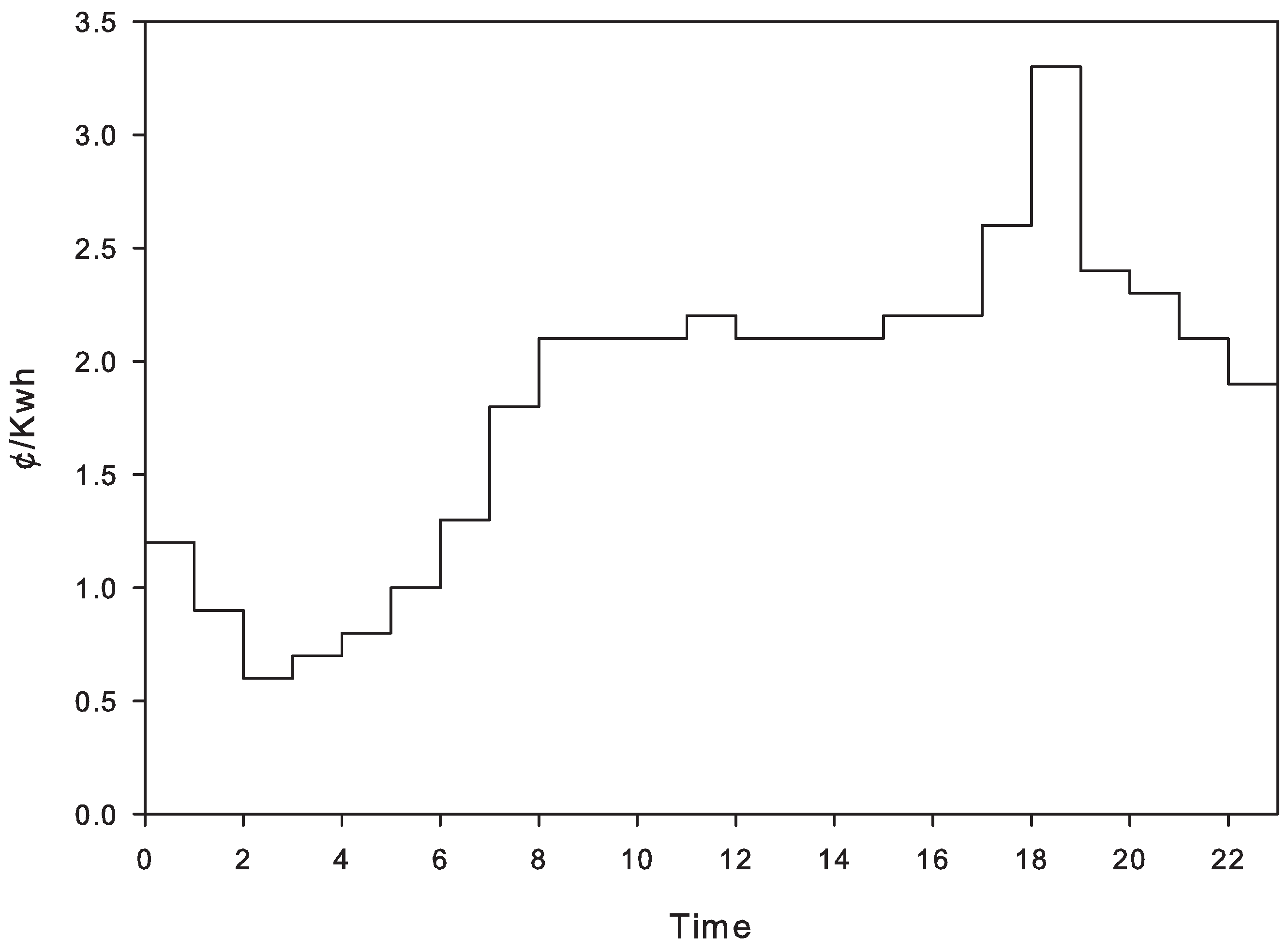
The values for the hourly pricing scheme are taken from [
26], and the exact used values can be seen in
Figure 4. This is one of the standard sources for such data and is also used in [
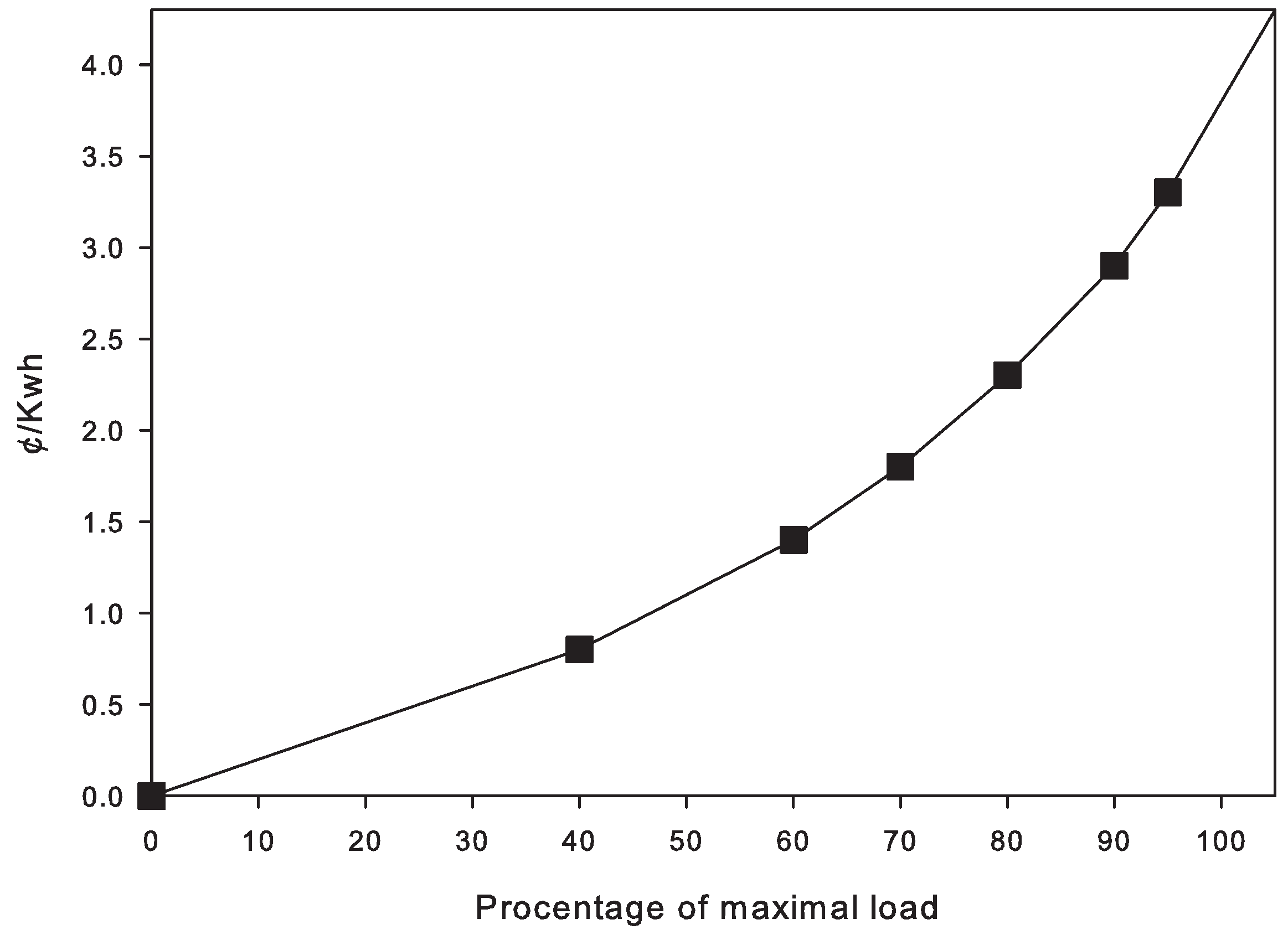
27]. Instead of a convex cost function, we use a linear piece-wise approximation, which is also commonly used in the literature. The exact values can be seen in
Figure 5. The maximal allowed load
L was equivalent to
-times the scaled value (to correspond to the number of households in test instance) of the monitored data.
Figure 4.
Hourly pricing program used for evaluating the proposed model. The data are taken from ComEd [
26].
Figure 4.
Hourly pricing program used for evaluating the proposed model. The data are taken from ComEd [
26].
Figure 5.
A piecewise linear convex cost function of instantaneous power consumption with seven consumption classes. Cross-over points are used to distinguish the classes.
Figure 5.
A piecewise linear convex cost function of instantaneous power consumption with seven consumption classes. Cross-over points are used to distinguish the classes.
4. Computational Experiments
In this section, we present the results of the performed computational experiments based on the proposed MIP formulation for the problem of interest. The model is implemented using IBM ILOG CPLEX Optimization Studio Version 12.6.1.0 (International Business Machines Corporation, New York, NY, USA) and executed using the default solver settings. The goal of the performed tests is to explore the trade-off between the household preference satisfaction and the production cost. Although we define the model using three objective functions, we investigate the Pareto front (PF) only for the bi-objective optimization problem using objectives and . The third goal is substituted by a constraint dependent on an input parameter.
For the simplified model, we calculate the approximate PF using the
ϵ-constraint method. In this method, a series of single objective optimization problems are solved. The other objective functions are substituted by constraints in the following way:
As is discussed in [
28], for bi-objective functions, this method can be used to calculate the PF with the additional effort of removing some dominated points.
In our computational experiments, we explore the relation between consumer comfort and production cost represented by two functions
,
. The experiments are conducted for problems with 50, 150 and 250 households. For each case, we observe that the PF for
. The computational time for all of the problem sizes is reasonable. On average, it took around
, 1 and
s to calculate one single objective problem for fixed values of
and
, for problems having 50, 150 and 250 households, respectively. The fixed values for
, corresponding to
ϵ in Equation (
17), used for calculating the PF were taken from the interval
with a step
. In practice, this meant that a maximum of 80 single objective optimization problems would be solved for calculating the PF for a fixed value of
. In the case of the problems containing 250 households, the PF is calculated within several minutes. It is noteworthy that, due to the consideration of appliance usage frequencies in the method for problem instance generation, a notable number (around 25%) of households (SP, SNP) has only one appliance. In practice, this has made solving the underlying combinatorial optimization problem less computationally expensive. The results of the computational experiments can be seen in
Figure 6.
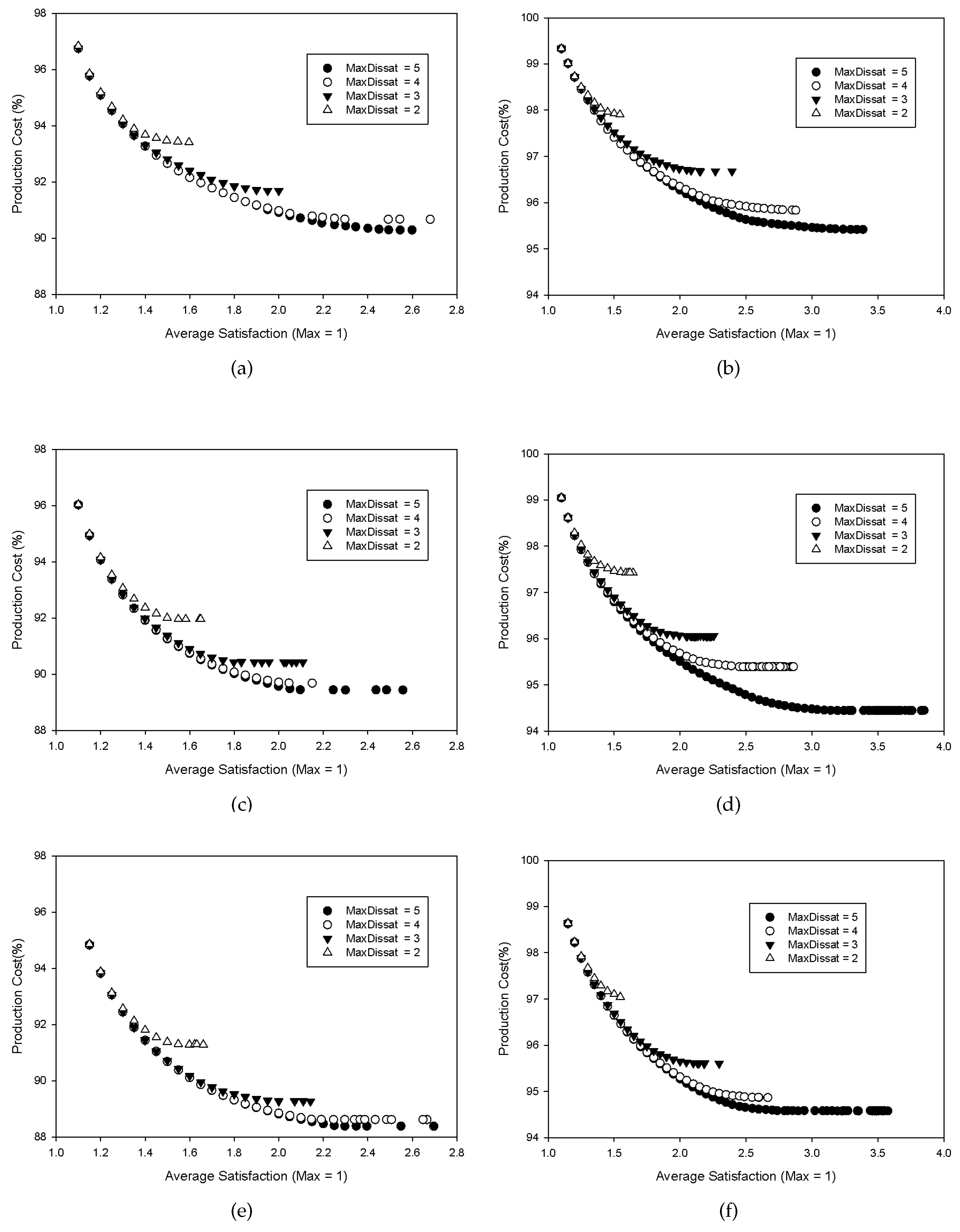
Figure 6.
The relation between average comfort levels and productions costs for a different number of households and the maximal allowed dissatisfaction levels. Production cost is defined as a linear approximation of a convex function (left) and using an hourly pricing scheme (right). Comfort levels vary between 1 and 6; Level 1 represents the maximum satisfaction, while Level 6 is the minimum satisfaction. (a)Pareto fronts (PFs) for 50 households using ; (b) PFs for 50 households using ; (c) PFs for 150 households using ; (d) PFs for 150 households using ; (e) PFs for 250 households using ; (f) PFs for 250 households using .
In the case of both objective functions,
Figure 6 shows the relative production cost (given in percent) compared to the one corresponding to the case when all appliances are used at the highest preference level (1). From the computational experiments, several conclusion can be made. First, an increase in the number of households that are scheduled together produces a higher level of savings. The results also indicate that increasing the number of households above a certain limit starts having a neglectful effect. This is similar to the original problem when satisfaction levels are not used. The potential savings are higher in the case that production costs are observed as a convex function for an hourly pricing scheme. In the case of the former, the savings have reached close to 12% in the case of 250 households for the lowest maximal allowed dissatisfaction levels. In the case of an hourly pricing scheme, the savings were less, and the highest level was lower than 6%. It is important to note that in the case of
, the savings are dependent on the selected convex function.
When observing the PF for the relation between the average household satisfaction levels and the production costs, several interesting conclusions can be made. The first is that decreasing the average satisfaction over a certain level has no effect on lowering the production cost for a red fixed maximal level of allowed dissatisfaction. Beyond this point, savings can only be achieved by reducing the allowed level of dissatisfaction. It is important to note that several percents of savings can be achieved only by reducing the maximal allowed dissatisfaction and maintaining the same average satisfaction. This can be exploited in defining pricing schemes for household groups. Another interesting aspect of the performed test is that even for a high average satisfaction (), more than 50% of potential savings are achieved if the maximal dissatisfaction is allowed to reach three.
5. Conclusions and Discussions
In this paper, a new model for scheduling demand response has been proposed. The model has taken the preferences of participating households into account and has been defined as a multi-objective optimization problem having objective functions corresponding to energy production costs and average household satisfaction. For the proposed model, a MIP has been developed. The model has been evaluated using real-world data based on the use of appliances in different types of households.
In the proposed model, customers can set up their preferences for each appliance, e.g., through smart energy management systems, and the scheduling system will continue to operate until the end of the day. If customers make any changes, they will be executed in the next day. Therefore, customers do not need to set the preference matrix each day, but they have to update it if necessary. The computational experiments have shown that coupling the consumers’ preference levels with the associated job descriptions can be beneficial, both for the customer and the utility company. To be exact, by giving this additional information, it is possible to achieve a significant level of savings in production costs while maintaining a high degree of satisfaction for the participating households. It has also been shown that by allowing a higher level of maximal dissatisfaction for households, further savings can be achieved. This type of information can be exploited in designing pricing models for consumers. The results also showed that the reduction in utility company operations can also be reflected in customer bills by means of incentives.
In the future, we are going to explore the potential of incorporating preference levels into an online version of the original problem, which will allow customers to be able to change their preferences during the day. We will also compare the two systems, online vs. offline, in terms of cost and customer satisfaction. Another direction of future research will be the extension of the model to a stochastic environment by further involving renewable generators and adapting it to a longer scheduling period.


