Parameter Identification Methods for Hyperelastic and Hyper-Viscoelastic Models

Abstract

In this paper, the Ogden model is employed to characterize the hyperelastic properties of rubber, and on the basis of a pattern search algorithm and the Levenberg-Marquardt algorithm, a professional method that can realize the comprehensive fitting of the uniaxial tension, biaxial tension, planar tension, and simple shear experimental data of hyperelastic materials was developed. The experiment data from Treloar (1944) was fitted very well, and the determined parameters by using this method were proven correct and practical in the numerical verification in ANSYS. Then, the constitutive model of the hyper-viscoelastic materials combining the Ogden model with the generalized Maxwell model was explained in detail, and the parameter identification method was also proposed by using the pattern search method. Then, three groups of relaxation tests of uniaxial tension and four groups of simple shear tests with different loading velocities were conducted to obtain the corresponding virtual experiment data. After discussing the constraints and initial setting values for the undetermined parameters, these virtual data of different loading histories were respectively employed to identify the parameters in the hyper-elastic model, and the accuracy and the reliability of the estimated parameters were also verified in ANSYS.

1. Introduction

With the rapid development of modern industrialization, rubbers are one of the most remarkable materials having a wide range of applications in civil engineering, aerospace engineering, mechanical engineering, automotive engineering, etc. In order to meet various requirements of the industry, special fillers, like carbon black or silica, with different proportions are usually added during vulcanization for improving the strength and toughness properties, which in turn makes it difficult to accurately characterize the mechanical a properties of rubbers [1]. Rubbers usually present a number of interesting features like hyperelasticity and hyper-viscoelasticity, many studies and experiments have been performed to investigate these features. For the former one, the stress-strain relationship of the hyperelasticity can be illuminated by a strain energy function W, and some mathematical models have been developed for the function, among which the strain-invariant-based models mainly include the Mooney-Rivlin model [2], the Yeoh model [3], and the Gent model [4], the principal-stretch-based models mainly include the Ogden model [5]. All the models have been verified by experiment results, for example Treloar’s experiment [6], and the Ogden model breaks through the limitation of the strain energy function being the even power of the stretches, which is capable of more accurately fitting the experimental data when rubbers undergo extremely large deformations. Comparisons of the performances of 20 hyperelastic models are presented in the article from Marckmann and Verron [7]. More detailed reviews on the hyperelasticity of rubber can be accessed in several literatures [8,9,10]. The identification of the parameters in theses hyperelastic models has also gained much attention. For example, Twizell and Ogden [11] employed the Levenberg-Marquardt optimization algorithm to determine the material constants in Ogden models, Saleeb et al. [12,13] developed a professional scheme named COMPARE to get the parameters by using uniaxial tension, biaxial tension, and planar tension data.

The constitutive relations for the viscoelasticity can be characterized by combining the elastic components with viscous components. In the past decades, numerous studies focused on investigating the viscoelasticity properties of rubber-like materials and many models explaining such behaviors were proposed. In the range of small strain, the basis of linear viscoelasticity theory was presented by Coleman et al. [14]. A relaxation-modulus constitutive function for the incompressible isotropic materials based on the results of uniaxial and equal biaxial stress relaxation tests was developed by McGuirt [15]. The phenomenological theory of linear viscoelasticity was proved powerful for modelling the static and dynamic responses of rubber when subjected to small strain [16,17]. For the finite deformation of viscoelastic materials, two important hypotheses were assumed. One is a split of the free energy of viscoelastic solid into an equilibrium and a non-equilibrium part, and the other one is a multiplicative decomposition of the deformation gradient tensor into elastic and inelastic parts [18]. In such a framework, Huber and Tsakmak is generalized the application range of the so-called three-parameter solids to the finite deformation [19]. Haupt et al. proposed a fairly simple identification method for the constants in a finite viscoelasticity model [20]. Yoshida et al. presented a constitutive model comprised by an elastoplastic body with a strain-dependent isotropic hardening law and a hyperelastic body with a damage model [21]. Amin et al. proposed an improved hyperelastic constitutive equation for rubbers in compression and shear regimes [1,22,23], the parameters in the equation were identified by experiment data and a nonlinear viscous coefficient was introduced to represent the rate-dependent properties. In recent years, a novel testing technique, named nanoidentation, to identify the material parameters for thin polymer layers was developed, a comprehensive review and the realization of the method for hyperelastic and viscoelastic models are presented by Chen et al. [24,25,26]

In this paper, the Ogden model is taken to characterize the hyperelastic properties of rubber-like materials. A professional method based on the pattern search algorithm (PSA) [27,28] and the Levenberg-Marquardt algorithm (LMA) [29] was developed to fit the unixial tension, biaxial tension, planar tension, and the simple shear experimental data of hyperelastic materials. Then, combining the generalized Maxwell model and the Ogden model as the constitutive model, the method that can identify the parameters in the hyper-viscoelastic models by using experimental data with different loading histories was also developed [24,25] and three groups of virtual relaxation tests and four groups of simple shear tests were employed to verify the accuracy and reliability of the proposed method.

2. Parameter Identification Method for the Hyperelastic Model

The constitutive models representing the hyperelastic properties of rubbers mainly include the statistical models, the strain-invariant-based models, and the principal-stretch-based models, among which the Ogden model is able to fit the experiment data when rubbers undergo large deformations ($\mathsf{\lambda }<7$). In the following sections, the parameter identification method for the hyperelastic model and the numerical verification of these identified parameters are presented in detail.

2.1. Theories of the Ogden Model

According to the theories of the continuum mechanics, there exists a strain energy function W for the hyperelasticity properties of rubbers. The stresses can be obtained by the partial derivative of the variable W with respect to the strain.

$$S=2\frac{\partial W}{\partial C}$$

(1)

where C is the right Cauchy-Green deformation gradient tensor, S is the second Piola-Kirchhoff stress.

After transforming the second Piola-Kirchhoff stress to the Cauchy stress [30], we will get

$$T=-pI+2\frac{\partial W}{\partial I_1}B-2\frac{\partial W}{\partial I_2}{B}^{-1}$$

(2)

where F is the deformation gradient tensor, B is the left Cauchy-Green deformation gradient tensor, $I_1,I_2,I_3$ are the three strain invariants of B, and p is the undetermined hydrostatic pressure which can be decided by the underlying equilibrium and boundary conditions of the particular problem.

In view of the nearly incompressible properties of the volume of rubbers, the strain energy of the Ogden model can be defined with Equation (3) without regard for the contribution of the volume strain.

$$W={\displaystyle \sum _n\frac{{\mathsf{\mu }}_n}{{\mathsf{\alpha }}_n}}({{\mathsf{\lambda }}_1}^{{\mathsf{\alpha }}_n}+{{\mathsf{\lambda }}_2}^{{\mathsf{\alpha }}_n}+{{\mathsf{\lambda }}_3}^{{\mathsf{\alpha }}_n}-3)$$

(3)

In Equation (3), n is the number of terms considered for the Ogden model, ${\mathsf{\mu }}_n$, ${\mathsf{\alpha }}_n$ are the undetermined parameters of the model, ${\mathsf{\lambda }}_i$ is the principal stretch.

In the uniaxial tension experiment, the deformation gradient tensor F and the left Cauchy-Green deformation gradient tensor B are described as

$$B=\left(\begin{array}{ccc}{{\mathsf{\lambda }}_1}^2& 0& 0\\ 0& 1/{\mathsf{\lambda }}_1& 0\\ 0& 0& 1/{\mathsf{\lambda }}_1\end{array}\right)$$

(4)

Taking the boundary condition $T_{22}=T_{33}=0$ into consideration, the corresponding nominal stress for uniaxial tension is

$$f_1=T_{11}/{\mathsf{\lambda }}_1={\displaystyle \sum _n{\mathsf{\mu }}_n}({{\mathsf{\lambda }}_1}^{{\mathsf{\alpha }}_n-1}-{{\mathsf{\lambda }}_1}^{-{\mathsf{\alpha }}_n/2-1})$$

(5)

For the biaxial tension experiment, the boundary conditions are $T_{22}=T_{33}$, $T_{11}=0$, ${\mathsf{\lambda }}_2={\mathsf{\lambda }}_3$, and the nominal stress is

$$f_2=T_{22}/{\mathsf{\lambda }}_2={\displaystyle \sum _n{\mathsf{\mu }}_n}({{\mathsf{\lambda }}_2}^{{\mathsf{\alpha }}_n-1}-{{\mathsf{\lambda }}_2}^{-2{\mathsf{\alpha }}_n-1})$$

(6)

The boundary condition of the planar tension experiment is $T_{33}=0,{\mathsf{\lambda }}_2=1$, and the nominal stress is

$$f_3=T_{11}/{\mathsf{\lambda }}_1={\displaystyle \sum _n{\mathsf{\mu }}_n}({{\mathsf{\lambda }}_1}^{{\mathsf{\alpha }}_n-1}-{{\mathsf{\lambda }}_1}^{-{\mathsf{\alpha }}_n-1})$$

(7)

As for the simple shear experiment, the direction of the principal stretch is not consistent with the direction of the applied deformation, rather it involves a rotation of axes [1]. The left Cauchy-Green deformation tensor B is expressed as

$$B=\left(\begin{array}{ccc}1+{\mathsf{\gamma }}^2& \mathsf{\gamma }& 0\\ \mathsf{\gamma }& 1& 0\\ 0& 0& 1\end{array}\right)$$

(8)

and the nominal shear stress is shown in Equation (9).

$$f_4=T_{12}=\frac{{\displaystyle \sum _n{\mathsf{\mu }}_n({{\mathsf{\lambda }}_1}^{{\mathsf{\alpha }}_n}-{{\mathsf{\lambda }}_1}^{-{\mathsf{\alpha }}_n})}}{{\mathsf{\lambda }}_1+1/{\mathsf{\lambda }}_1}$$

(9)

where the principal stretch ${\mathsf{\lambda }}_1$ can be obtained by calculating the eigenvalues of the tensor B.

$${\mathsf{\lambda }}_1=\sqrt{1+\frac{{\mathsf{\gamma }}^2}{2}+\mathsf{\gamma }\sqrt{1+\frac{{\mathsf{\gamma }}^2}{4}}}$$

(10)

2.2. The Object Function for Parameter Identification

Previous studies have shown that the constitutive parameters of a hyperelastic model identified from a particular deformation mode may be invalid for other modes. For example, Charlton et al. claimed that the parameters identified from the uniaxial test data fail in predicting biaxial or planar tension responses [31]. So, it is of much significance to take the four types of experiment data listed above into consideration. This goal can be achieved by the least square procedure to make the deviations of the experiment data and the fitted data least. The object function is defined as

$$min:S_1={\displaystyle \sum _{q=1}^4{\mathsf{\omega }}_q}({\displaystyle \sum _{i=1}^{n_q}{({(f_q)}_i-{({\mathsf{\sigma }}_q)}_i)}^2})$$

(11)

where ${\mathsf{\omega }}_q$ is the weight of different experiment type, if there exists no experiment data for a specific type, we just need to set its ${\mathsf{\omega }}_q$ to be zero, if we want to emphasize the experiment data of a specific type, we can set its ${\mathsf{\omega }}_q$ larger than others’. $n_q$ represents the number of the experiment data for each type of experiment, ${(f_q)}_i$ is the theoretical value which is calculated by Equations (5)–(7) and (9), ${({\mathsf{\sigma }}_q)}_i$ is the experiment data.

2.3. The Identified Parameters and the Numerical Verification

In this paper, the uniaxial tension, biaxial tension, and planar tension data from Treloar are taken as the experiment data [6], and the Ogden model is chosen as the hyperelastic model owing to its favorable performances under large deformations. In order to solve Equation (11), the PSA is employed as the first step for its remarkable ability in searching for the global optimum results. Then, the L-M algorithm is chosen to further optimize the results from the first step due to the probable poor efficiency of the PSA when approaching the optimum results. All the procedures are realized in MATLAB [32].

The number of terms considered for the Ogden model are respectively set as three and four, and seven groups of different initial values of undetermined parameters for each one are iterated in parallel. For the limited space and the similarity between the results of different groups, only the ones with the least iterations and its corresponding deviation S₁ are chosen and listed in

Table 1. Results of the identified parameters in Ogden model.

Iterations	Treloar	N = 3		N = 4
		PSA 169000+	LMA 48	PSA 280000+	LMA 65
${\mathsf{\mu }}_1$	0.6174	0.37282	0.45262	0.64979	0.806
${\mathsf{\mu }}_2$	0.001176	1.0209 × 10−5	2.642×10−5	0.027261	0.0327533
${\mathsf{\mu }}_3$	−0.0098	8.2746×10−3	−0.01191	0.0032134	2.3601×10−7
${\mathsf{\mu }}_4$	-	-	-	−0.0095667	−0.004861
${\mathsf{\alpha }}_1$	1.3	1.8464	1.60617	1.13221	0.80939
${\mathsf{\alpha }}_2$	5	7.29012	5.70992	4.526	8.9157
${\mathsf{\alpha }}_3$	−2	−2.09521	−1.98197	1.1313	3.19726
${\mathsf{\alpha }}_4$	-	-	-	−2.0548	−2.26312
S1	0.106	0.0618	0.0333	0.0598	0.0120

PSA: pattern search algorithm; LMA: Levenberg-Marquardt algorithm.

. The estimated parameters presented by Treloar are presented as well [6]. The unit of ${\mathsf{\mu }}_{\mathrm{i}}$ in Table 1 is Mpa, and the item ‘PSA 169000+’ means more than 169 thousand iterations in PSA, and the ‘LMA 48’ means 48 iterations in LMA after the previous PSA procedure. Moreover, the computation time for the whole procedure with an i7 CPU is about 6 h.

As the Table 1 shows, these three groups of parameters are all capable of fitting the experiment data very well, and the last group is the best owing to its least deviation 0.012., However, despite thousands of iterations of the PSA and LMA, the two sets of the identified parameters in Table 1 may not be the optimal results of Equation (12), because there may be local minimum points extremely close to the global minimum one, and these local optimal points have not been excluded by the PSA for their relatively excellent, not merely most excellent, competitions and they are identified by the LMA. Even so, these identified parameters, being optimal or near-optimal, are still very useful due to enough accuracy and controlled computation cost. Additionally, It should be mentioned that the PSA takes more than 200 thousand iterations to reduce the S₁ from 0.1 to 0.0598, while the LMA only takes 65 iterations to reduce the deviation from 0.06 to 0.012, which strongly reflects the inefficiency of the PSA when approaching the global optimal point, and taking the LMA as a succeeding procedure to further optimize results is practical and efficient. In the last iteration of the LMA, the sensitivity values for the items $\partial S/\partial {\mathrm{u}}_i$ and $\partial S/\partial {\mathsf{\alpha }}_i$ are all more than 10⁹, which means accurate estimations of all the parameters.

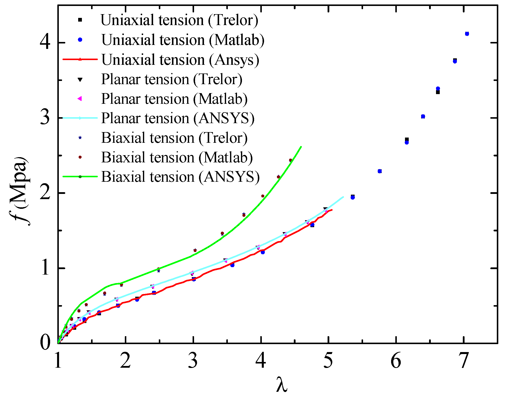
For the purpose of verifying the estimated parameters, the last group of the identified parameters is taken as the example to predict the response of rubbers in different types of experiments in ANSYS. The results of the numerical simulation, the fitted data obtained by the use of the proceeding algorithm, along with the experiment data from Treloar are all plotted in Figure 1.

As illustrated in the Figure 1, the results identified by the PSA and LMA fit the experiment data very well. Besides, in the numerical simulation tests, the results of uniaxial tension and planar tension coincide well with the experiment data (when the principal stretch is larger than 5, the FE analysis of uniaxial tension tests cannot converge due to some uncertain reasons). However, the results of biaxial tension tests differ a bit from the experiment data, the reason for the errors lies in that the boundary conditions of the biaxial tension experiment cannot be accurately satisfied when the principal stretch ranges from 1.5 to 1.9 in the simulation test.

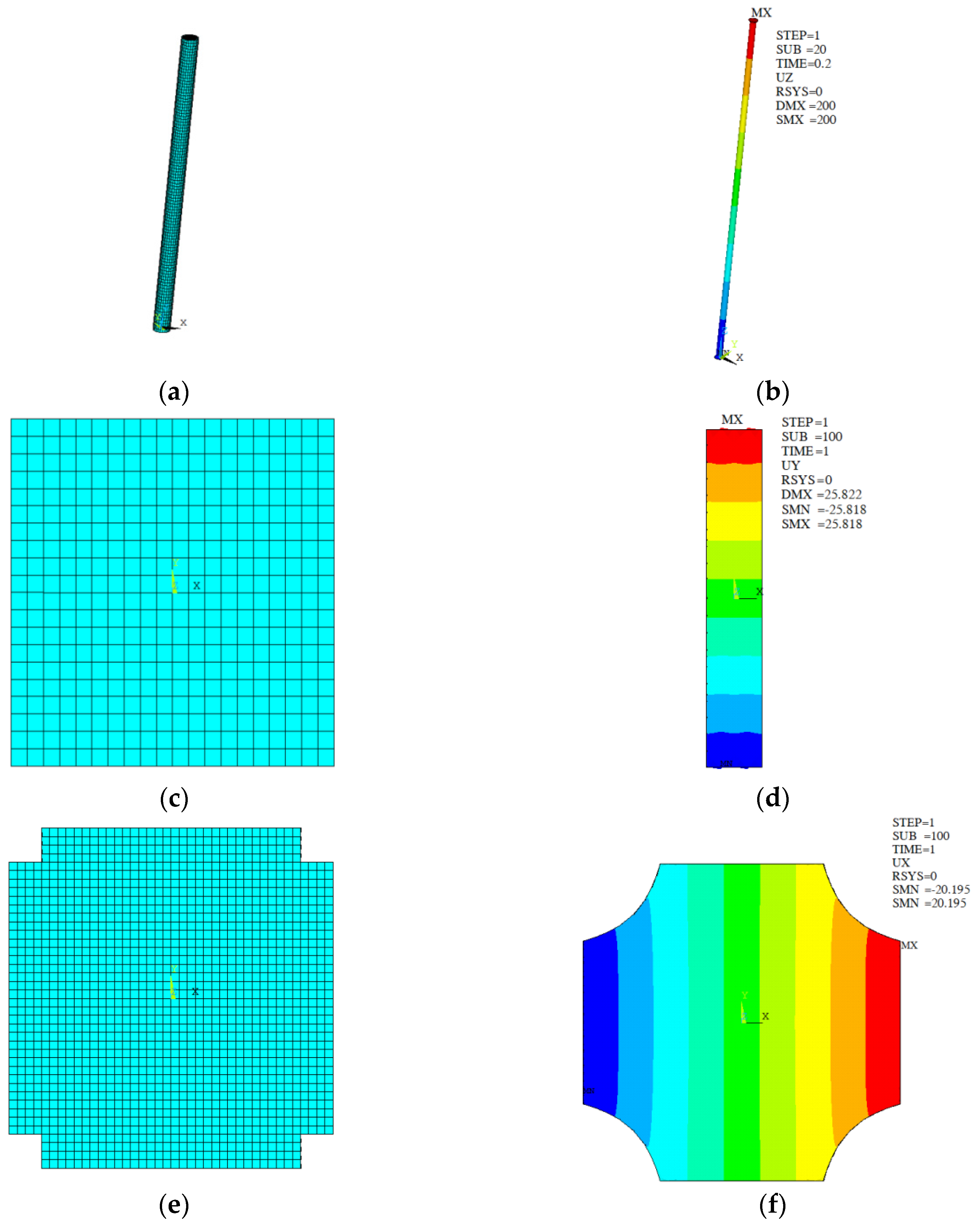
The FE initial models of uniaxial tension, planar tension, and biaxial tension experiment and their deformed shapes with the stretch being 5, 6.14, and 5.04 are presented respectively in Figure 2.

3. Parameter Identification Method for the Hyper-Viscoelastic Model

In the previous section, the parameter identification method for the hyperelastic model was explained in detail, this model is suitable for the numerical simulation of natural rubbers with low damping. As for the high damping rubbers, they can be simulated by combining the Ogden model with the generalized Maxwell model. In the following, theories of the hyper-viscoelastic model and the parameter identification method for the model were expounded.

3.1. Theories of the Hyper-Viscoelastic Model

The integration of the relaxation modulus for viscoelasticity is expressed in Equation (12)

$$\mathsf{\sigma }(t)={\displaystyle {\int }_{-\infty }^{t}Y(t-\mathsf{\xi })}d\mathsf{\epsilon }(\mathsf{\xi })$$

(12)

where $Y(t-\mathsf{\xi })$ is the relaxation modulus function for characterizing the viscoelastic properties, and $d\mathsf{\epsilon }(\mathsf{\xi })$ is the micro-strain of materials. Generally, when $\mathsf{\xi }<0$, the outer action is assumed to be 0, so Equation (12) will be changed to

$$\mathsf{\sigma }(t)={\displaystyle {\int }_0^{t}Y(t-\mathsf{\xi })}d\mathsf{\epsilon }(\mathsf{\xi })$$

(13)

Equation (13) can be calculated by dividing the time t into n equal portions, then we will get

$$\mathsf{\sigma }(t)={\displaystyle \sum _{i=1}^n{\displaystyle {\int }_{t_i}^{t_{i+1}}Y(t-\mathsf{\xi })d\mathsf{\epsilon }(\mathsf{\xi })}}$$

(14)

When $\mathsf{\xi }\in (t_i,t_{i+1})$, the Young modulus of materials is assumed to be a constant $E_i$, and the Prony series is introduced to characterize the relaxation properties. Besides, the strain loading speed is also deemed as a constant ${\mathsf{\lambda }}_i$, then Equation (14) will become

$$\mathsf{\sigma }(t)={\displaystyle \sum _{i=1}^n{\displaystyle {\int }_{t_i}^{t_{i+1}}{\mathsf{\lambda }}_i{E}_i({\mathsf{\mu }}_0+{\displaystyle \sum _{k=1}^m{\mathsf{\mu }}_k}{e}^{-(t-\mathsf{\xi })/t_k})d\mathsf{\xi }}}$$

(15)

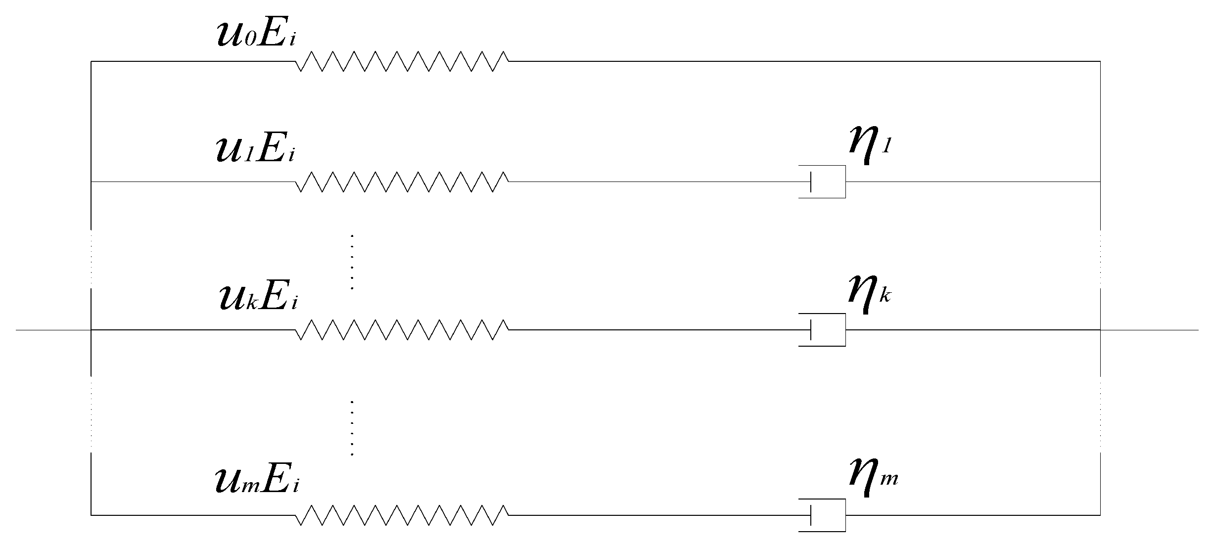
where ${\mathsf{\mu }}_k$ is the weight of modulus corresponding to the relaxation time $t_k$, m is the number of terms considered for the Prony series, ${\mathsf{\mu }}_0$ is the weight of the equilibrium modulus. It is obvious for the equation ${\displaystyle \sum _{k=0}^m{\mathsf{\mu }}_k}=1$ to be true, and the physical model of Equation (15) is presented in Figure 3.

In Figure 3, $E_i$, ${\mathsf{\mu }}_0$, ${\mathsf{\mu }}_k$ shares the same meaning with that in Equation (15), ${\mathsf{\eta }}_k$ represents the viscosity coefficient and ${\mathsf{\eta }}_k={\mathsf{\mu }}_k{E}_i{t}_k$, $t_k$ is the relaxation time included in Equation (15).

This physical model includes two main features, the first one is that it substitutes the stretch-dependent modulus spring for the constant modulus spring of the generalized Maxwell model, which is based on an assumption that the modulus corresponded to the viscosity coefficient ${\mathsf{\eta }}_k$ is obtained by multiplying the instantaneous modulus $E_i$ and the weight $u_k$. The second one is that the instantaneous modulus $E_i$ can be decided by the hyperelasticity properties of materials, and the weight $u_k$ is the undetermined parameters which are time independent.

If we stipulate that $t_k={10}^{k-1}{t}_1$, which is adopted by the FE software LS-DYNA [33], then, $\mathsf{\sigma }(t)$can be expressed as

$$\mathsf{\sigma }(t)={\displaystyle \sum _{i=1}^n{\displaystyle {\int }_{t_i}^{t_{i+1}}{\mathsf{\lambda }}_i{E}_i({\mathsf{\mu }}_0+{\displaystyle \sum _{k=1}^m{\mathsf{\mu }}_k}{e}^{-(t-\mathsf{\xi })/({10}^{k-1}{t}_1)})d\mathsf{\xi }}}$$

(16)

As mentioned before, $E_i$ represents the instantaneous modulus of materials within the time range from $t_i$ to $t_{i+1}$. It can be solved by the following procedures. Firstly, the fast stretch-stress experiment data is obtained by conducting experiment at sufficiently high speed to exclude the viscous effect. Then they will be fitted by the Ogden model to decide the undetermined parameters, which has been explained in the previous section. After acquiring the stretch-stress curve based on the Ogden model, $E_i$ will be solved by the derivation of the stress $\mathsf{\sigma }$ with respect to the principal stretch $\mathsf{\lambda }$, namely, ${\left(\frac{\partial \mathsf{\sigma }}{\partial \mathsf{\lambda }}\right)}_{t=t_i}$, or taking the secant modulus as a substitution for the tangent modulus, namely, $({\mathsf{\sigma }}_{i+1}-{\mathsf{\sigma }}_i)/({\mathsf{\lambda }}_{i+1}-{\mathsf{\lambda }}_i)$.

3.2. The Parameter Identification Algorithm for the Hyper-Viscoelastic Model

According to Equation (16), the number of the undetermined parameters is m + 1, including $u_k$ and $t_1$. Similarly to Equation (11), the object function for the parameter identification of hyper-viscoelastic model can be defined as follows,

$$min:S_2={\displaystyle \sum _{j=1}^p{\displaystyle \sum _{i=1}^{n_j}{(f_i-T_i)}^2}}$$

(17)

where p represents the number of the tests with different loading histories, $n_j$ is the number of the experiment data for the jth group of experiment, $T_i$ is the experiment data, $f_i$ is the theoretical value which is calculated by Equation (16).

In order to get the global optimum results for the undetermined parameters in Equation (17), the global optimal searching algorithm, namely pattern search algorithm, is also employed in this section.

3.3. Different Loading Histories and Virtual Experiment Data

Similarly, with the identification in the Section 2.2, it is necessary to incorporate different loading histories to guarantee the accuracy of the identified multi-parameters in Equation (17). Hence, the relaxation tests of uniaxial tension and the simple shear tests with different loading velocities are taken as examples in this study. Due to the lack of appropriate data for these experiments, we followed the method applied in Chen et al. [24,25,26] and got the corresponding virtual experiment data by using ANSYS, in which we assume the hyperelastic parameters are the same with the last group in Table 1, and the viscoelastic part is characterized by the following Prony series,

$$P(\mathsf{\xi })=0.4e^{-(t-\mathsf{\xi })/10}+0.1e^{-(t-\mathsf{\xi })/100}$$

(18)

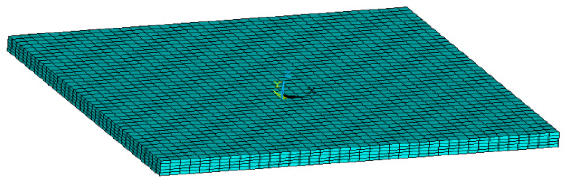
In the virtual experiment, the finite element (FE) model for the relaxation tests is identical with that in Figure 2a, and the model for the simple shear tests is illustrated in Figure 4. All the material constants are determined by the above discussions.

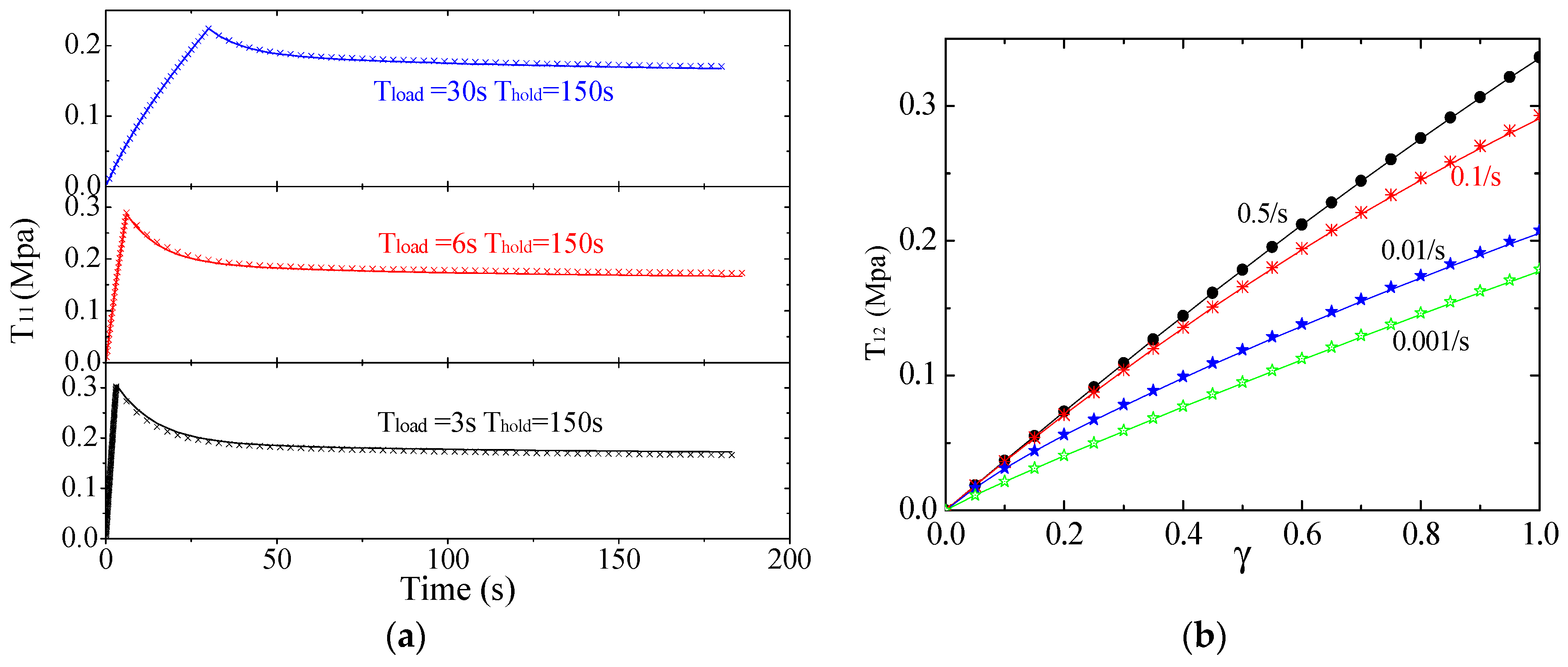
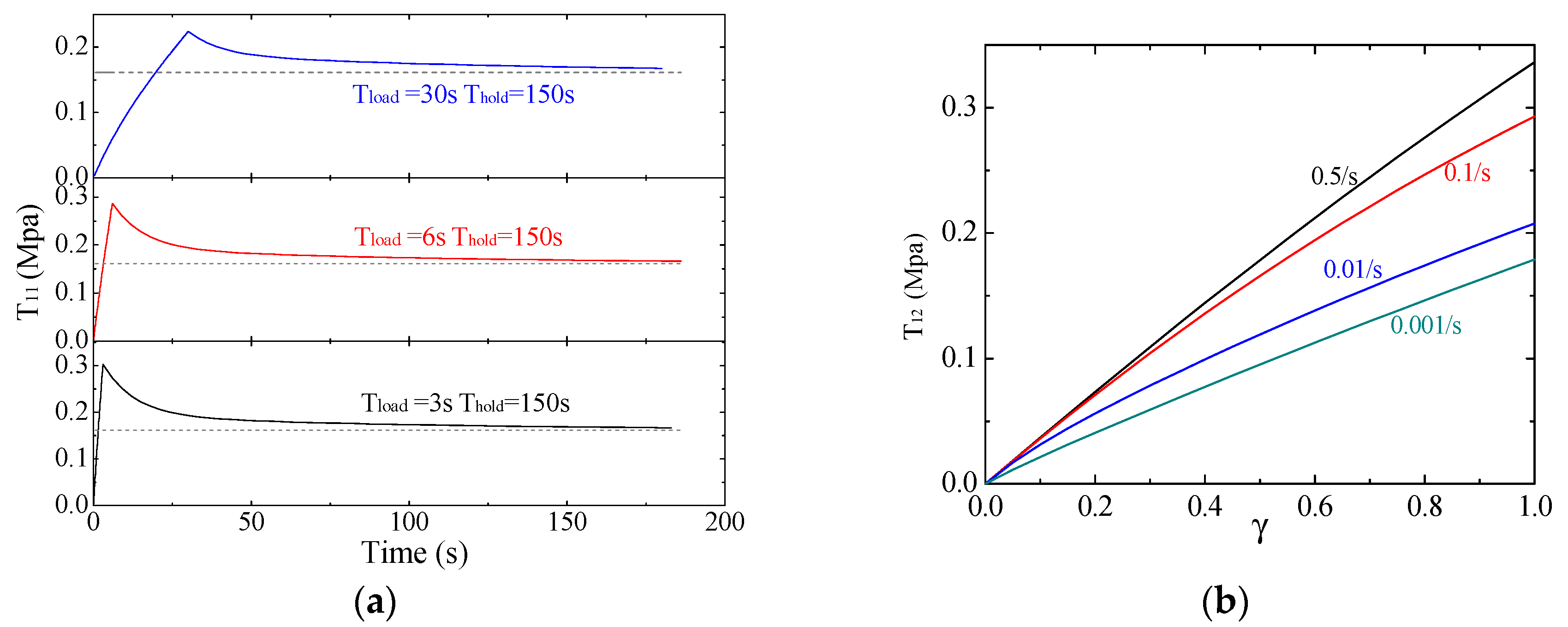
Then, three groups of data for relaxation tests and four groups of simple shear experiment data with different loading velocities are obtained. As shown in Figure 5, the maximum stretch is 1.3 in the relaxation tests with the loading time being respectively 3 s, 6 s, and 30 s, and the hold time being 150 s. For the simple shear tests, the maximum shear strain is 1.0 with the loading velocities being 0.5/s, 0.1/s, 0.01/s, and 0.001/s.

3.4. Constraints and Initial Values of Parameters

Before presenting results, it is necessary to clarify the constraints as well as the initial setting values for the undetermined parameters in the identified procedure. As for the weight $u_k$, as well as the summation of all $u_k$ except $u_0$, they should be always within the range from 0 to 1. While for the relaxation time $t_1$, it should be positive and a suggested initial value is the main relaxation time of materials, which can be determined by the point corresponding to the relaxed stress ${\mathsf{\sigma }}_{0.368}$ in creep tests, here the ${\mathsf{\sigma }}_{0.368}$ is defined as

$${\mathsf{\sigma }}_{0.368}=0.368({\mathsf{\sigma }}_0-{\mathsf{\sigma }}_{\infty })+{\mathsf{\sigma }}_{\infty }$$

(19)

in which the ${\mathsf{\sigma }}_0$ is the instantaneous stress and the ${\mathsf{\sigma }}_{\infty }$ is the equilibrium stress.

The creep experiment of the material characterized by Equation (18) and the last group of parameters in Table 1 is conducted in ANSYS, and the main relaxation time is 12.54 s.

As for the number of the terms considered for the Prony series, theoretically, the experiment data in Figure 5 will be more accurately fitted with a higher number, however, this may lead to uncontrolled computation cost and sometimes unreasonable estimated parameters. In this study, the number to be decided is suggested to make the largest relaxation time in Equation (16) the same order of magnitude with the largest experiment time. For example, the largest experiment time in Figure 5 is 1000 s, so, the number of the terms considered for the Prony series is 3 since the corresponding largest relaxation time now is 1254 s.

In view of all the restrictions presented above, as well as the consideration of testing the reliability of the pattern search algorithm, four groups of initial values for the undetermined parameters are presented in

Table 2. The initial values for undetermined parameters.

Group	${\mathit{t}}_{\mathbf{1}}$/s	${\mathit{u}}_{\mathbf{1}}$	${\mathit{u}}_{\mathbf{2}}$	Group	${\mathit{t}}_{\mathbf{1}}$/s	${\mathit{u}}_{\mathbf{1}}$	${\mathit{u}}_{\mathbf{2}}$	${\mathit{u}}_{\mathbf{3}}$
1	12.54	0.1	0.05	3	12.54	0.1	0.05	0.01
2	30	0.7	0.2	4	30	0.7	0.2	0.05

. Besides, taking the third group as an example, the linear constraint equations for the parameters during iterations are shown in Equation (20).

$${\left[\begin{array}{ccccccccc}1& 0& 0& 0& 0& -1& 0& 0& 0\\ 0& 1& 0& 0& 1& 0& -1& 0& 0\\ 0& 0& 1& 0& 1& 0& 0& -1& 0\\ 0& 0& 0& 1& 1& 0& 0& 0& -1\end{array}\right]}^T\left[\begin{array}{c}{t}_1\\ u_1\\ u_2\\ u_3\end{array}\right]<{\left[\begin{array}{ccccccccc}100& 1& 1& 1& 1& 0& 0& 0& 0\end{array}\right]}^T$$

(20)

3.5. Results and Discussions

3.5.1. Uniaxial Relaxation Tests

The identified parameters by each group of relaxation test are presented in

Table 3. The identified parameters by the uniaxial relaxation tests.

	Tload (s) = 3 s					Tload (s) = 6 s
Group	$t_1$/s	$u_1$	$u_2$	$u_3$	S2	$t_1$/s	$u_1$	$u_2$	$u_3$	S2
	10	0.4	0.1	0		10	0.4	0.1	0
1	11.564	0.405	0.088	-	9.23 × 10−5	10.917	0.399	0.093	-	3.53 × 10−5
2	11.578	0.405	0.087	-	9.24 × 10−5	11.025	0.399	0.093	-	3.53 × 10−5
3	11.718	0.409	0.0698	0.0706	9.07 × 10−5	11.025	0.403	0.075	0.075	3.53 × 10−5
4	11.651	0.408	0.072	0.072	9.07 × 10−5	11.081	0.404	0.0735	0.0734	3.44 × 10−5
	Tload (s) = 30 s
Group	$t_1$/s		$u_2$	S2	Group	$t_1$/s	$u_1$	$u_2$	$u_3$	S2
	10	0.4	0.1			10	0.4	0.1	0
1	9.643	0.395	0.093	2.99 × 10−5	3	9.753	0.399	0.0755	0.0765	2.87 × 10−5
2	9.648	0.395	0.093	2.99 × 10−5	4	9.759	0.399	0.0754	0.0764	2.87 × 10−5

. The original values for the undetermined parameters $t_1$, $u_1$, $u_2$, and $u_3$ are respectively 10, 0.4, 0.1, and 0.

As shown in Table 3, all the groups with different loading histories and initial values are able to identify the parameters in the hyper-viscoelastic models. The identified weight in each group is nearly identical with its original one, while the weights $u_2$, and $u_3$ in some groups, are a bit poorly determined. For the identified relaxation time $t_1$, it becomes more accurate with the increasing of the loading time T_load, and in the group of the T_load being 30 s, the identified relaxation time is about 3.6% lower than its true value. Subsquently, the deviation S₂ of each group decreases as the T_load increases with the least one being 2.87×10⁻⁵. Besides, for the results with the same loading time, the identified parameters are little affected by the initial setting value and the number of terms for the Ogden model, which indicates a strong reliability of the PSA.

3.5.2. Simple Shear Tests

For the four groups of simple shear experiment data in Figure 5, they are not employed separately like the relaxation tests, instead all data with different shear velocities are combined together to determine the global optimal results. Similarly, the PSA is utilized and the identified parameters are shown in

Table 4. The identified parameters by simple shear tests.

Group	${\mathit{t}}_{\mathbf{1}}$/s	${\mathit{u}}_{\mathbf{1}}$	${\mathit{u}}_{\mathbf{2}}$	S2	Group	${\mathit{t}}_{\mathbf{1}}$/s	${\mathit{u}}_{\mathbf{1}}$	${\mathit{u}}_{\mathbf{2}}$	${\mathit{u}}_{\mathbf{3}}$	S2
	10	0.4	0.1			10	0.4	0.1	0
1	9.547	0.403	0.1004	1.31 × 10−5	3	9.544	0.4030	0.1001	−0.001	1.3 × 10−5
2	9.546	0.403	0.1004	1.31 × 10−5	4	9.5235	0.4025	0.1016	−0.001	1.3 × 10−5

.

It can be seen from Table 4 that the parameters in different groups are almost the same with each other, and the weights u₁ and u₂ are almost accurately identified with the relaxation time a bit deviated from its true value. However, an abnormal negative value −0.001, extremely close to 0, of the weight u₃ is observed even though we have set constraints for all the weights as shown in Equation (20), this unusual phenomenon may be an indication of the weight u₃ redundant for the problem.

3.5.3. Verification of the Identified Results

In order to verify the accuracy of the estimated parameters, one out of the four groups of the identified parameters in Table 3 and Table 4 are employed in ANSYS to predict the corresponding responses of the hyper-viscoelastic materials. Comparisons of the results calculated by ANSYS and the data in Figure 5 are plotted in Figure 6.

In Figure 6, the solid line represents the original data and the scatter points represent the results from ANSYS by using the identified parameters. It is obvious that errors in every experiment are very small, which means the proposed analytical model for hyper-viscoelastic materials and the identification method by using PSA are reliable and efficient.

4. Conclusions

In this study, we focused on the parameter identification of the hyperelastic and hyper-viscoelastic materials, and the following conclusions have been made:

• Based on the pattern search algorithm and the Levenberg Marquardt algorithm, the comprehensive fitting of the multi-type experiment data of hyperelastic models, including uniaxial tension, planar tension, biaxial tension, and simple shear experiment have been realized.
• According to the fitting results of the experiment data from Treloar (1944) and the verification results of the numerical simulation, the method of combining the pattern search algorithm and Levenberg Marquardt algorithm proposed in this paper for identifying parameters in the Ogden model is practical and efficient.
• The parameter identification method for the hyper-viscoelastic materials which is characterized by combing the Ogden model with the generalized Maxwell model was developed, and the physical model of the hyper-viscoelastic model was also presented.
• Three groups of relaxation tests and four groups of simple shear tests were conducted in ANSYS and the corresponding experiment data were obtained. After employing the data to determine the parameters, it can be concluded that the proposed analytical model of the hyper-viscoelastic model and the identification method by using a pattern search algorithm is reliable since all the experiment data are fitted very well with extremely low deviations, and the identified results are little affected by the initial values as well as the term considered for Maxwell models.