
Quantitative Assessment of Variational Surface Reconstruction from Sparse Point Clouds in Freehand 3D Ultrasound Imaging during Image-Guided Tumor Ablation


Abstract
:
1. Introduction
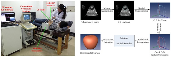
1.1. Freehand 3D Ultrasound Imaging
1.2. Volume Reconstruction for Freehand 3D Ultrasound Imaging
1.3. Surface Reconstruction for Freehand 3D Ultrasound Imaging
1.4. Contribution and Structure of this Paper
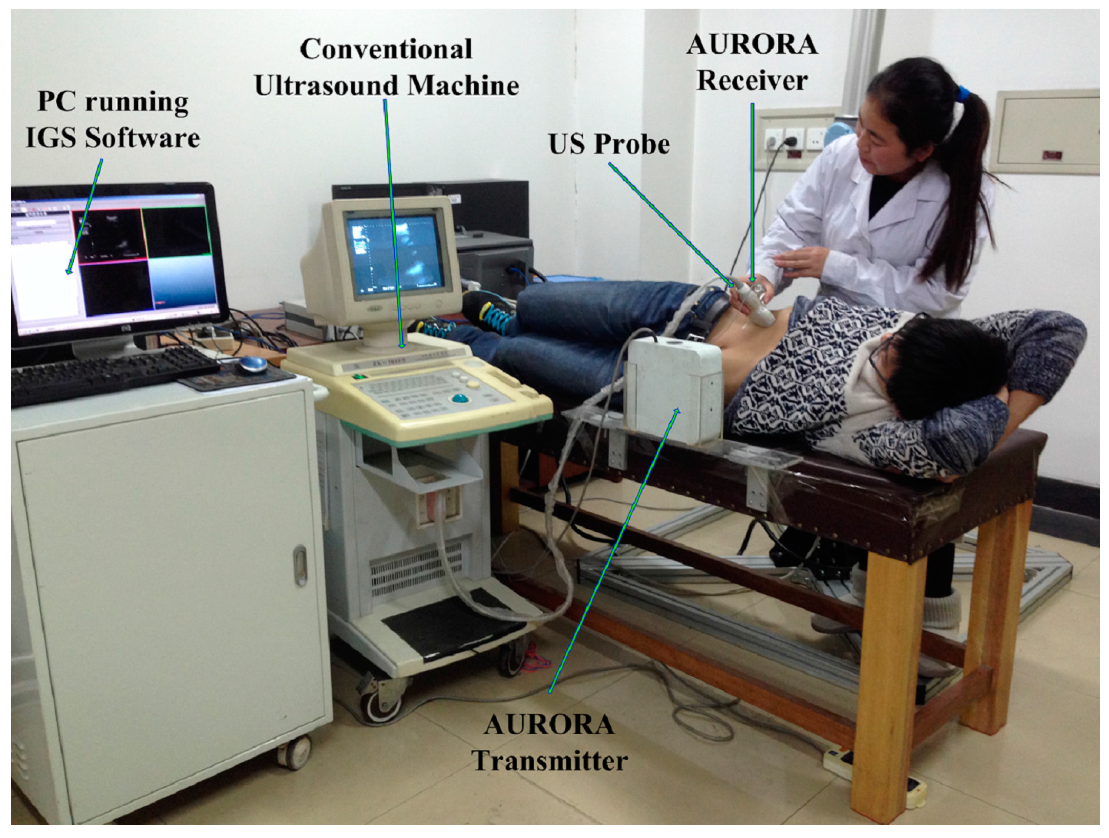
2. Framework of Surface Reconstruction for Freehand 3D US Using VSR
3. Four Methods of Surface Reconstruction from Point Clouds
3.1. VSR
3.1.1. Constraint Definition
- Step 1:
- Begin with the first contour. Mark it as the current contour.
- Step 2:
- For each point of the current contour, assign a scalar value 0 to . After the assignment, becomes an on-surface constraint .
- Step 3:
- For each point of the current contour, calculate its corresponding off-surface constraint according to Equations (1) and (2).
- Step 4:
- When all the points of the current contour are finished, go to the next contour. Mark it as the current contour.
- Step 5:
- Loop from step 2 to step 4 until all contours are finished.
3.1.2. Variational Interpolation
- Step 1:
- For any pair of constraints and , calculate
- Step 2:
- After all pairs of and are calculated, form the coefficient matrix A in Equation (3):
- Step 3:
- Calculate vector B using Equation (4). Each denotes the corresponding value assigned to the constraint point .
- Step 4:
- Solve Equation (5). The solution vector v contains the weights dj of and the coefficients of .
3.2. Ball Pivoting
3.3. Power Crust
3.4. Poisson Reconstruction
4. Quantitative Metrics for Assessment of Surface Reconstruction
- mean distance (mean)
- standard deviation from the mean distance (std)
- root mean square distance (rms)
- maximum distance (Hausdorff)
- medial distance (median).
5. Experiments
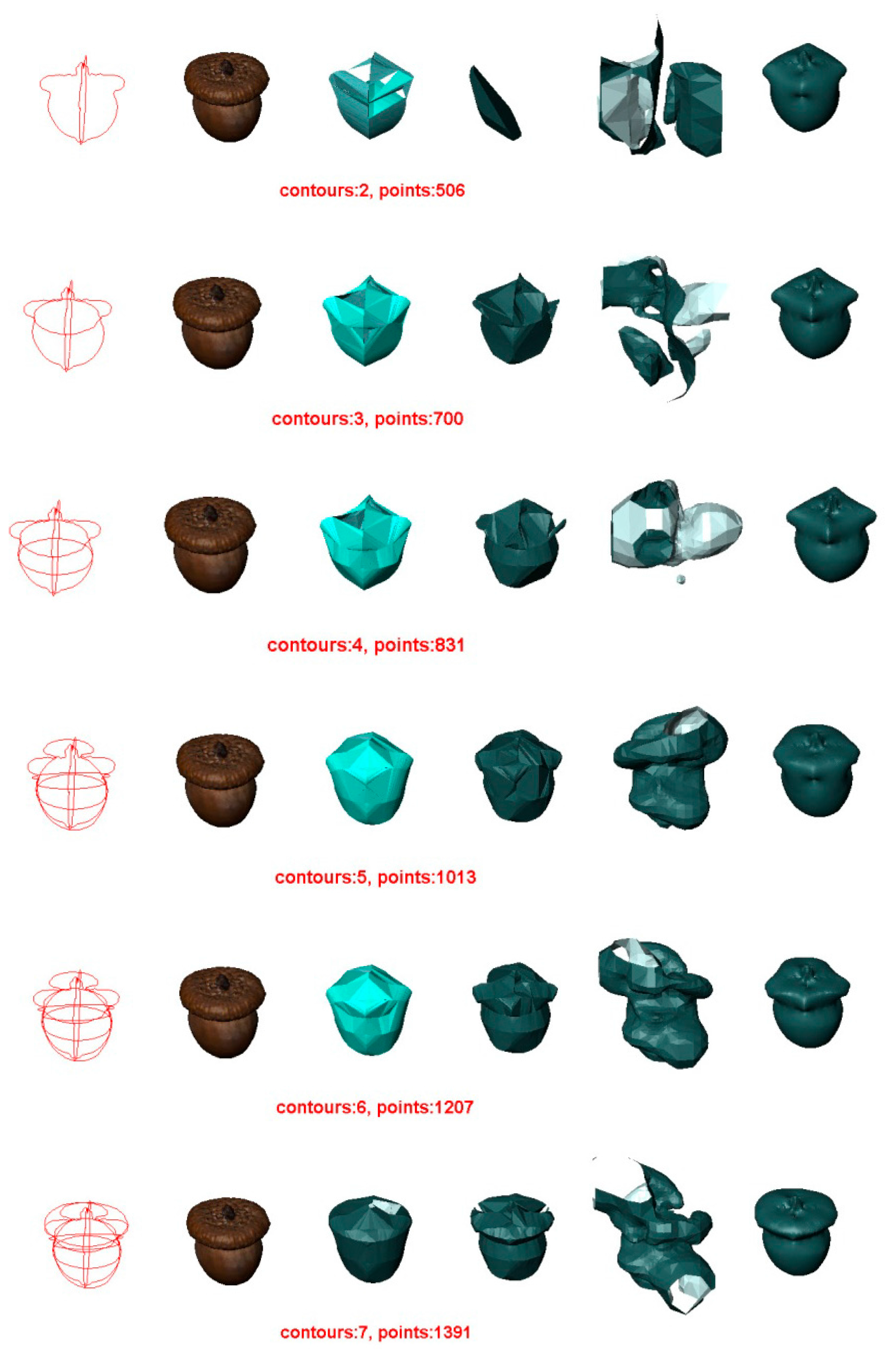
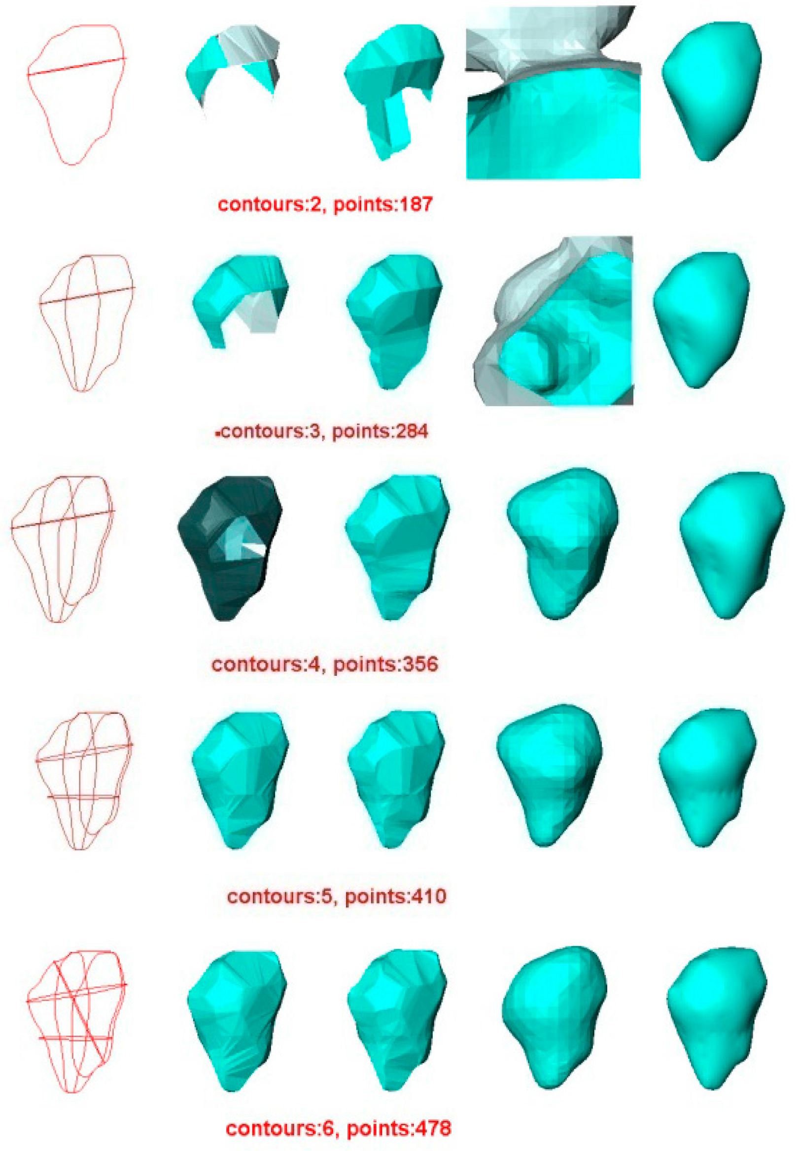
5.1. Experiment 1—Reconstruction of Acorn
- In all cases, the surface reconstructed by the VSR method best visually resembles the original surface compared with the other methods. Most metrics show that the VSR-reconstructed surface shows fewer differences from the original surface compared with the other methods. The only exception is observed in volume difference for four contours, where the Poisson method produces a volume that is more similar to the original surface than that of the VSR method.
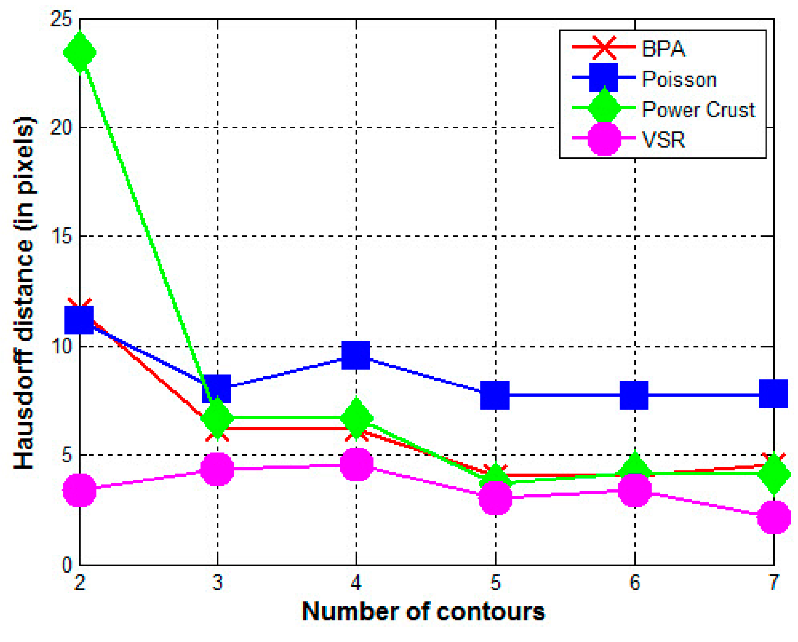
- For the other three methods, the quality of the reconstructed surfaces drops dramatically as the number of contours decreases (as seen for two or three contours in Figure 4 and Figure 5). However, as the number of contours decreases, both the quality and the Hausdorff distance for the VSR method show little variation. Even with only two contours, the VSR surface reconstruction closely approximates the original surface.
- Visually and quantitatively, the Poisson method performs the worst, except when reconstructed with two contours. Although Poisson and VSR are implicit-function-based methods, the Poisson method fails to reconstruct a satisfactory surface in all cases.
- Although the Power Crust method claims to be capable of producing watertight surfaces, it fails to do so when it is performed on two contours. This makes it the worst method for surface reconstruction with only two contours.
- As an intuitive and efficient method, BPA succeeds in constructing a triangle mesh for all cases. When the input data are dense (i.e., seven contours), it can produce a satisfactory surface of the acorn. However, its performance decreases dramatically as the number of contours decreases.
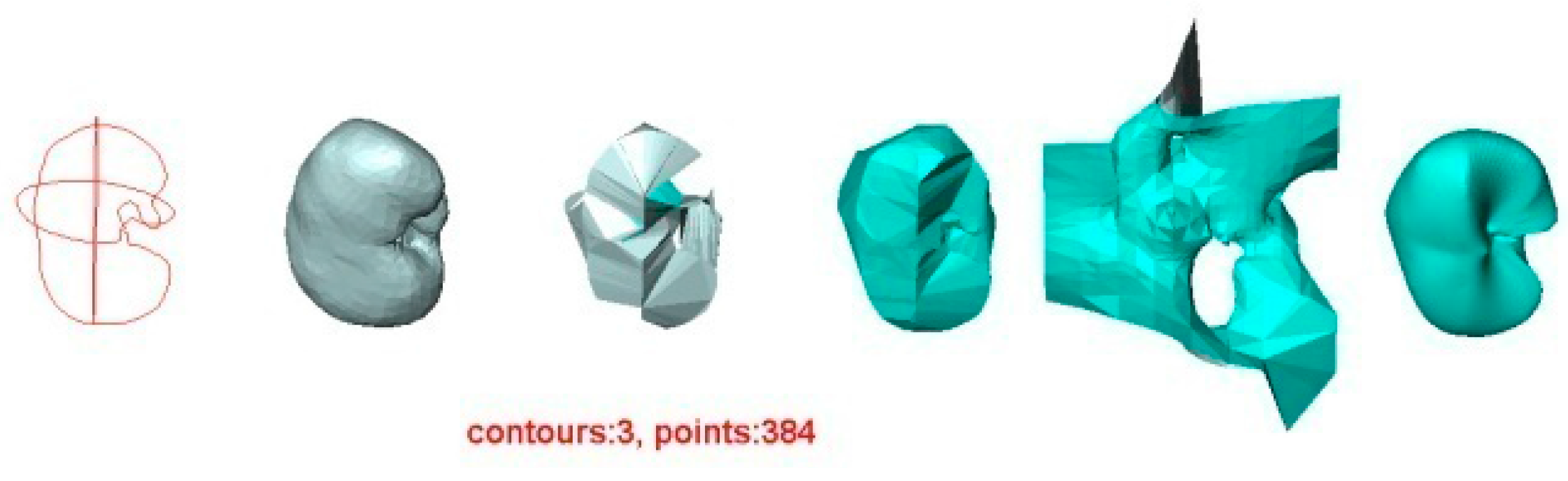
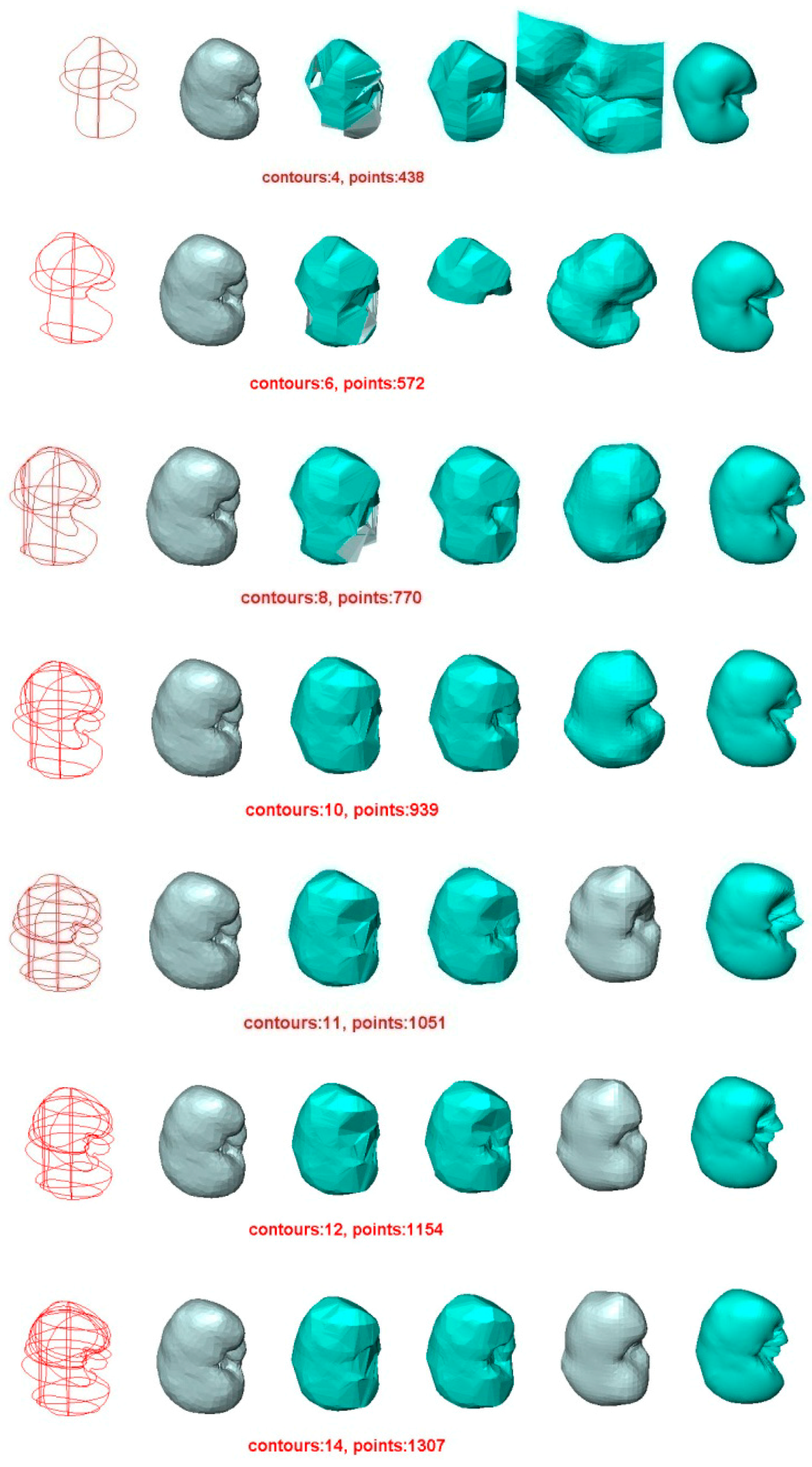
5.2. Experiment 2—Reconstruction of Human Kidney
5.3. Experiment 3—Reconstruction of Liver Tumor
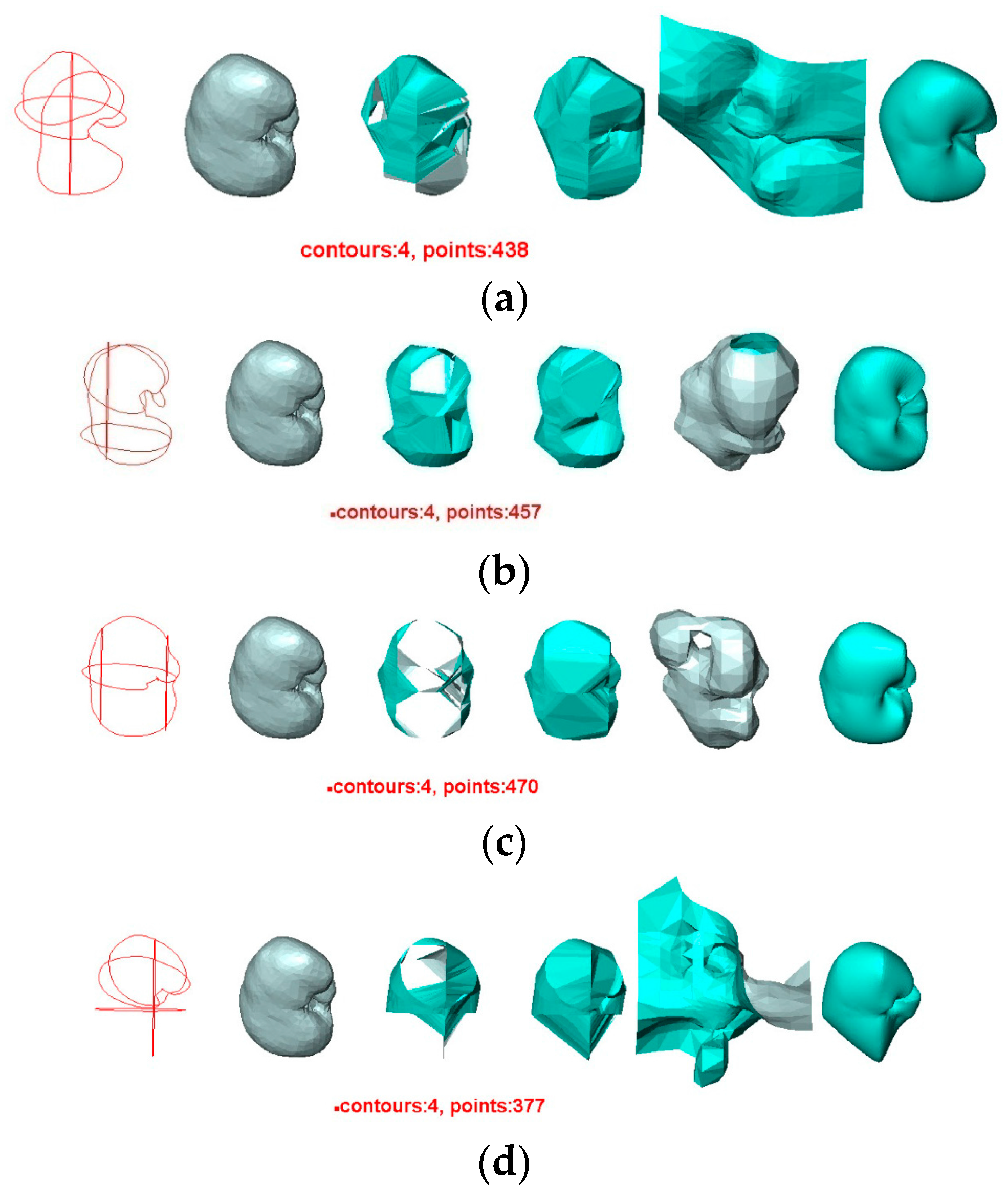
5.4. Experiment 4—Assessing the Reproducibility of Four Methods
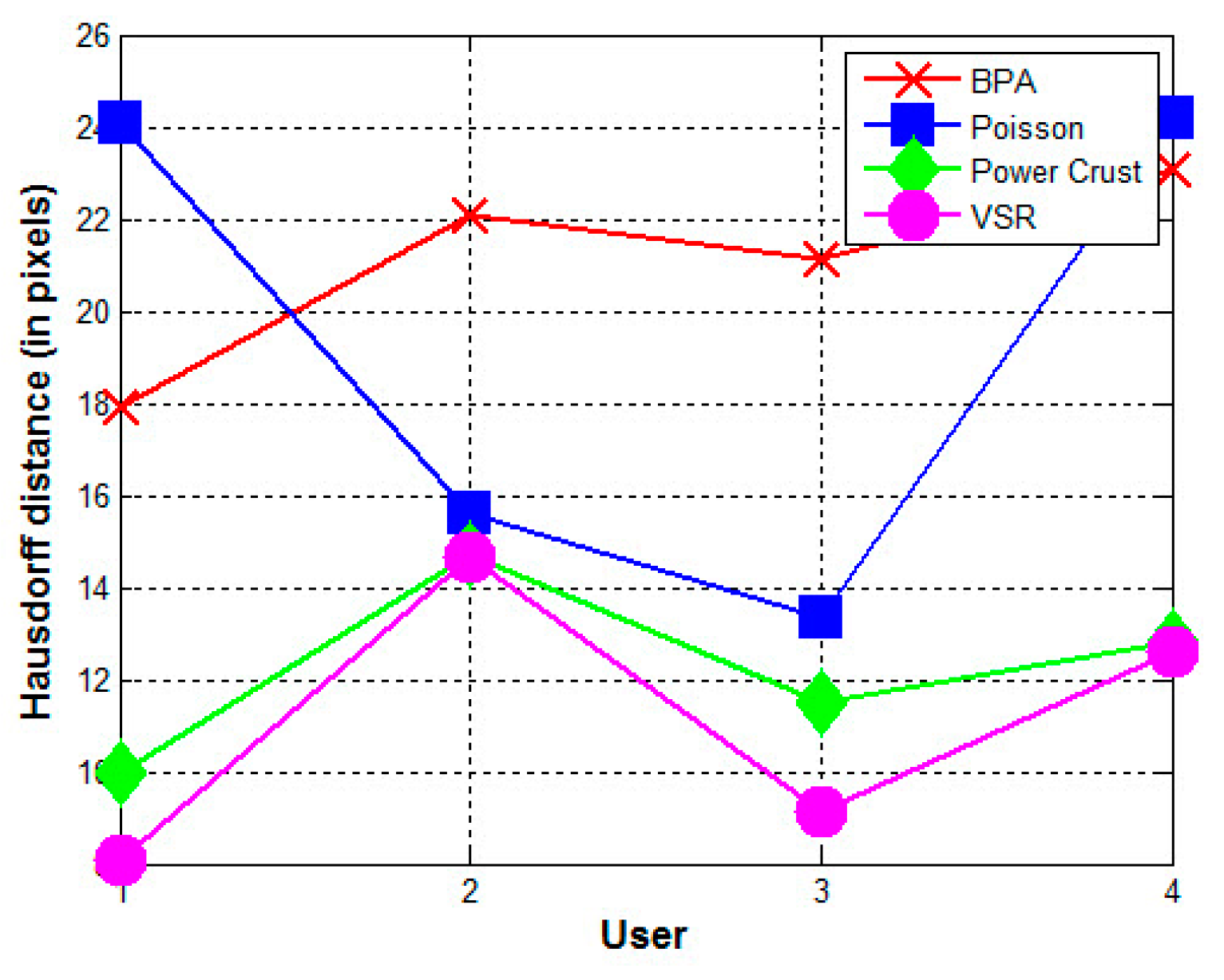
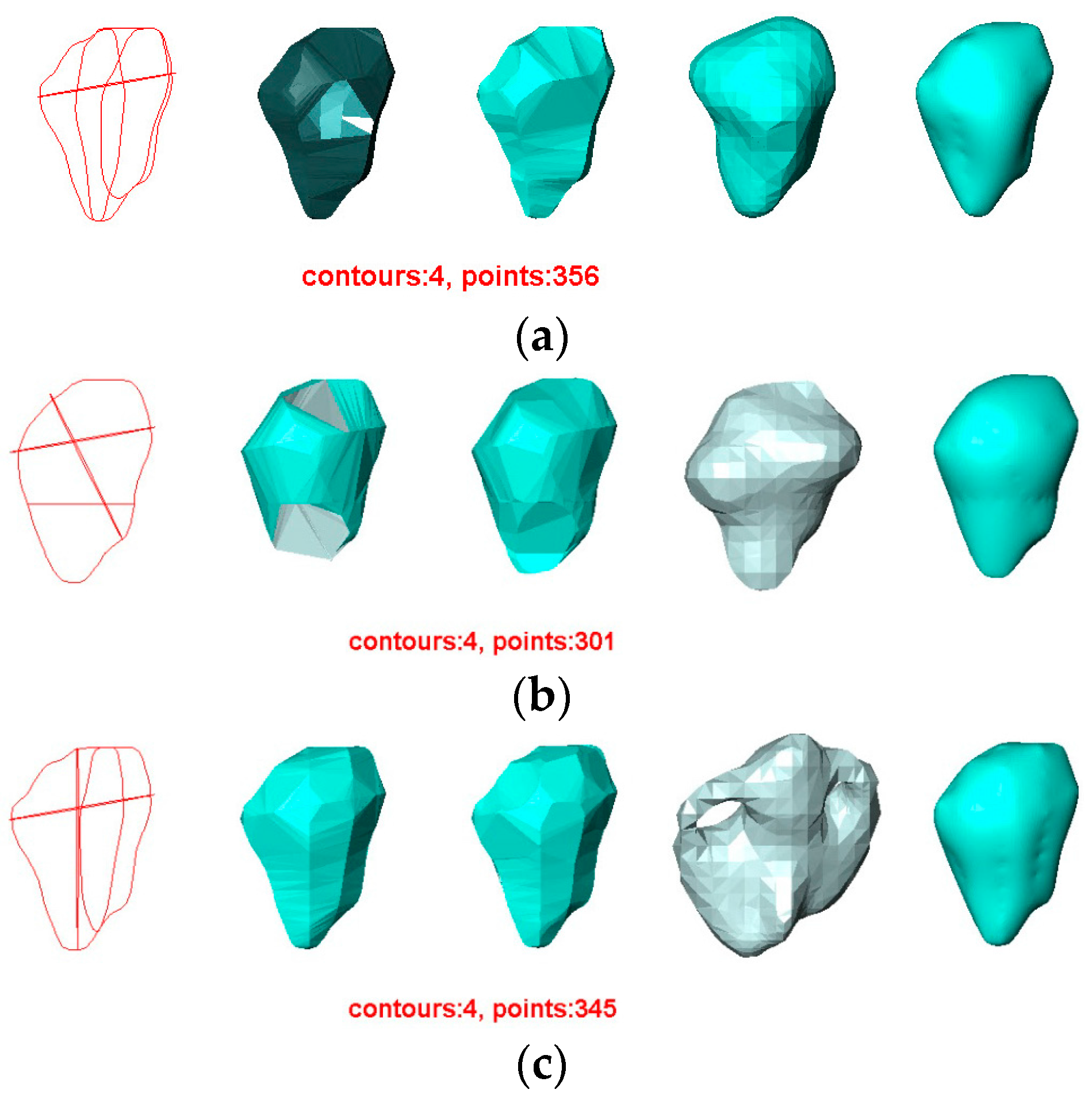
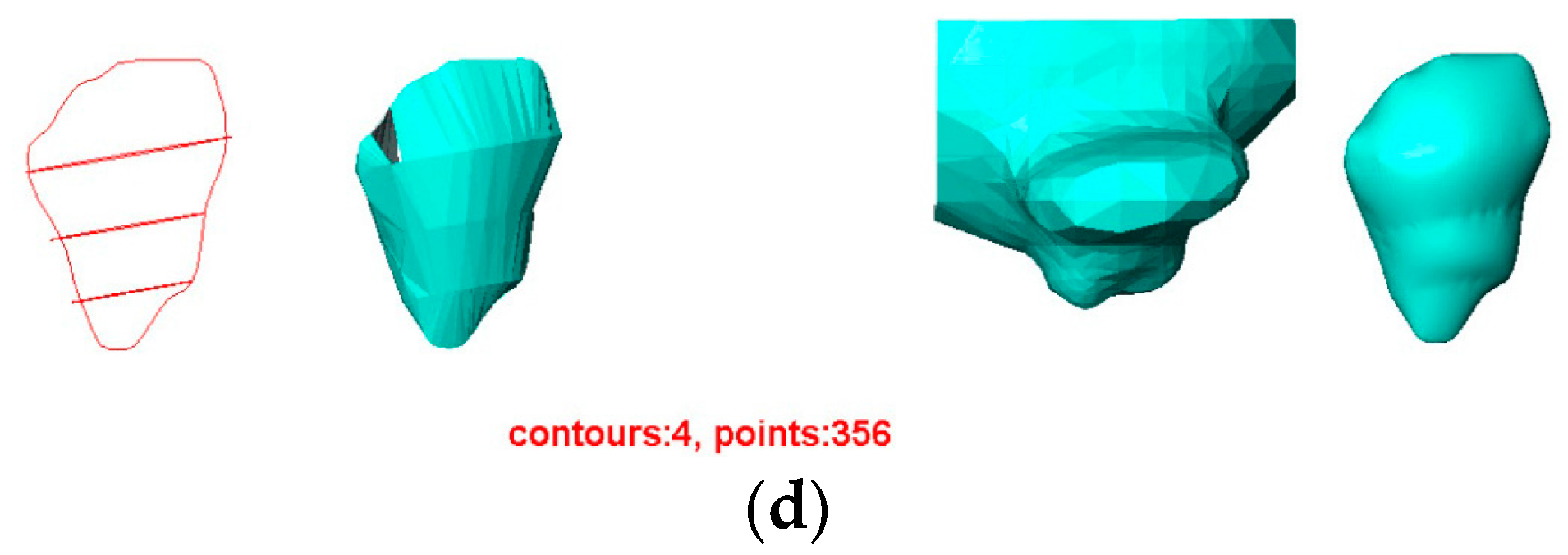
- The contours used greatly affect the quality of the reconstructed surfaces by all four methods. Visually, the contours drawn by User 3 produce the best approximation to the original surface, and the contours drawn by User 4 produce the poorest. Figure 11 confirms this conclusion graphically. This result indicates that the sparse input contours should cover the key contours of the original surface to produce a close approximation to it.
- In all cases, the surface reconstructed by the VSR method best visually resembles the original surface compared with the other methods. All metrics show that the VSR-reconstructed surface shows fewer differences from the original surface compared with the other methods, which indicates that the reproducibility of the VSR method is the best of the four methods.
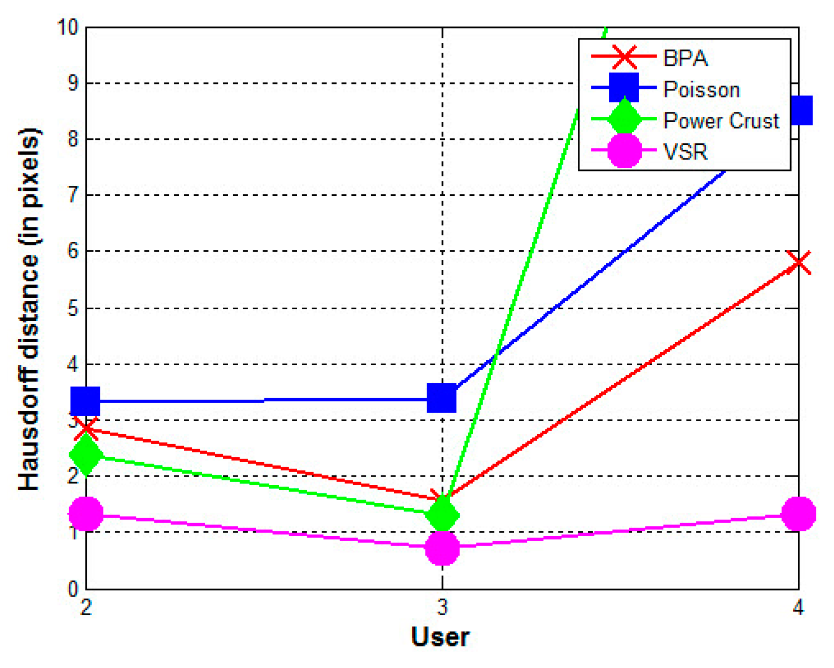
- The contours used greatly affect the quality of the reconstructed surfaces by all four methods. Visually, the contours drawn by User 3 produce the best approximation to the reconstructed surface from the contours drawn by User 1 using the BPA, Power Crust, and VSR methods. The contours drawn by User 4 produce the poorest approximation, especially when the Power Crust method is used; it fails to produce a surface. Figure 13 confirms this conclusion graphically. It should be noted that the Hausdorff distance of the Power Crust method is missing in Figure 13 since its value is much greater than that of the other methods.
- In all cases, the surface reconstructed by the VSR method best visually resembles the original surface compared with the other methods. All metrics show that the VSR-reconstructed surfaces show fewer differences from the surface reconstructed from the contours drawn by User 1 compared with the other methods, which indicates that the reproducibility of the VSR method is the best of four methods.
6. Discussion
7. Conclusions
Acknowledgments
Author Contributions
Conflicts of Interest
References
- Zhao, W.P.; Han, Z.Y.; Zhang, J.; Liang, P. A retrospective comparison of microwave ablation and high intensity focused ultrasound for treating symptomatic uterine fibroids. Eur. J. Radiol. 2015, 84, 413–417. [Google Scholar] [CrossRef] [PubMed]
- Livaghi, T.; Goldberg, S.N.; Lazzaroni, S.; Meloni, F.; Ierace, T.; Solbiati, L.; Gazelle, G.S. Hepatocellular carcinoma: Radio-frequency ablation of medium and large lesions. Radiology 2000, 214, 761–768. [Google Scholar] [CrossRef] [PubMed]
- Liu, F.Y.; Yu, X.L.; Liang, P.; Cheng, Z.G.; Han, Z.Y.; Dong, B.W.; Zhang, X.H. Microwave ablation assisted by a real-time virtual navigation system for hepatocellular carcinoma undetectable by conventional ultrasonography. Eur. J. Radiol. 2012, 81, 1455–1459. [Google Scholar] [CrossRef] [PubMed]
- Reis, J.; Butani, D. Tumor Ablation: Ultrasound versus CT. Ultrasound Clin. 2013, 8, 171–183. [Google Scholar] [CrossRef]
- Reis, J.; Butani, D. Ultrasound Guidance in Tumor Ablation. Ultrasound Clin. 2014, 9, 67–79. [Google Scholar] [CrossRef]
- Huang, X.; Hill, N.A.; Peters, T.M. Ultrasound-based technique for intrathoracic surgical guidance. In Proceedings of the Medical Imaging 2005: Visualization, Image-Guided Procedures, and Display, San Diego, CA, USA, 12 February 2005.
- Fenster, A.; Downey, D.B. 3-D ultrasound imaging—A review. IEEE Eng. Med. Biol. Mag. 1996, 15, 41–51. [Google Scholar] [CrossRef]
- Fenster, A.; Downey, D.B.; Cardinal, H.N. Three-dimensional ultrasound imaging. Phys. Med. Biol. 2000, 46, R67–R99. [Google Scholar] [CrossRef]
- Gee, A.; Prager, R.; Treece, G.; Berman, L. Engineering a freehand 3D ultrasound system. Pattern Recognit. Lett. 2003, 24, 757–777. [Google Scholar] [CrossRef]
- Mercier, L.; Langø, T.; Lindseth, F.; Collins, L.D. A review of calibration techniques for freehand 3-D ultrasound systems. Ultrasound Med. Biol. 2005, 31, 143–165. [Google Scholar] [CrossRef] [PubMed]
- Rousseau, F.; Hellier, P.; Barillot, C. Confhusius: A robust and fully automatic calibration method for 3D freehand ultrasound. Med. Image Anal. 2005, 9, 25–38. [Google Scholar] [CrossRef] [PubMed]
- Rao, Y.; Li, X.X.; Jiang, L.P.; Deng, S.C.; Cao, Y.Y.; Yao, P.; Li, X.H.; Liu, S.Q. 3-D calibration method for freehand ultrasound image with high precision based on string-beads phantom. In Proceedings of the Industrial Mechatronics and Automation (ICIMA), 2010 2nd International Conference on, Wuhan, China, 30–31 May 2010.
- Solberg, O.V.; Lindseth, F.; Torp, H.; Blake, R.E.; Hernes, T.A.N. Freehand 3D Ultrasound Reconstruction Algorithms—A Review. Ultrasound Med. Biol. 2007, 33, 991–1009. [Google Scholar] [CrossRef] [PubMed]
- Rohling, R.; Gee, A.; Berman, L. A comparison of freehand three-dimensional ultrasound reconstruction techniques. Med. Image Anal. 1999, 3, 339–359. [Google Scholar] [CrossRef]
- Prager, R.; Gee, A.; Treece, G.; Berman, L. Freehand 3D ultrasound without voxels: Volume measurement and visualisation using the Stradx system. Ultrasonics 2002, 40, 109–115. [Google Scholar] [CrossRef]
- Sherebrin, S.; Fenster, A.; Rankin, R.N.; Spence, D. Freehand three-dimensional ultrasound: Implementation and applications. In Proceedings of the Medical Imaging 1996: Physics of Medical Imaging, Toronto, ON, Canada, 10 February 1996; pp. 296–303.
- Barry, C.D.; Allott, C.P.; John, N.W.; Mellor, P.M.; Arundel, P.A.; Thomson, D.S.; Waterton, J.C. Three dimensional freehand ultrasound: Image reconstruction and volume analysis. Ultrasound Med. Biol. 1997, 8, 1219–1224. [Google Scholar] [CrossRef]
- Scheipers, U.; Koptenko, S.; Falco, T.; Remilinger, R.; Lachaine, M. 3-D Ultrasound Volume Reconstruction Using the Direct Frame Interpolation Method. IEEE Trans. Ultrason. Ferroelectr. Freq. Control 2010, 57, 2460–2470. [Google Scholar] [CrossRef] [PubMed]
- William, L.; Harvey, E.C. Marching cubes: A high resolution 3-d surface construction algorithm. Comput. Gr. 1987, 4, 163–169. [Google Scholar]
- Newman, T.S.; Yi, H. A survey of the marching cubes algorithm. Comput. Gr. 2006, 30, 854–879. [Google Scholar] [CrossRef]
- Suri, J.S.; Liu, K.; Singh, S.; Laxminarayan, S.N.; Zeng, X.; Reden, L. Shape recovery algorithms using level sets in 2-D/3-D medical imagery: A state-of-the-art review. IEEE Trans. Inf. Technol. Biomed. 2002, 6, 8–28. [Google Scholar] [CrossRef] [PubMed]
- Poon, M.; Hamarneh, G.; Abugharbieh, R. Efficient Interactive 3D Livewire Segmentation of Objects with Arbitrarily Topologies. Comput. Med. Imaging Gr. 2008, 32, 639–650. [Google Scholar] [CrossRef] [PubMed]
- Mory, B.; Ardon, R.; Yezzi, A.; Thiran, J.-P. Non-Euclidean Image-Adaptive Radial Basis Functions for 3D Interactive Segmentation. In Proceedings of the IEEE 12th International Conference on Computer Vision, Kyoto, Japan, 29 September–2 October 2009; pp. 787–794.
- Grady, L. Random Walks for Image Segmentation. IEEE Trans. Pattern Anal. Mach. Intell. 2006, 28, 1768–1783. [Google Scholar] [CrossRef] [PubMed]
- Boykov, Y.; Funka-Lea, G. Graph Cuts and Efficient N-D Image Segmentation. Int. J. Comput. Vis. 2006, 70, 109–131. [Google Scholar] [CrossRef]
- Cook, L.T.; Cook, P.N.; Lee, K.R.; Batnitzky, S.; Wong, B.Y.S.; Fritz, S.L.; Ophir, J.; Dwyer, S.J.; Bigongiari, L.R.; Templeton, A.W. An algorithm for volume estimation based on polyhedral approximation. IEEE Trans. Biomed. Eng. 1980, 9, 493–500. [Google Scholar] [CrossRef] [PubMed]
- King, D.L.; Gopal, A.S.; Keller, A.M.; Sapin, P.M.; Schröder, K.M. Three-dimensional echocardiography: Advances for measurement of ventricular volume and mass. Hypertension 1994, 1, I172–I179. [Google Scholar] [CrossRef]
- Hodges, T.C.; Detmer, P.R.; Burns, D.H.; Beach, K.W.; Strandness, D.E., Jr. Ultrasonic three-dimensional reconstruction: In vitro and in vivo volume and area measurement. Ultrasound Med. Biol. 1994, 20, 719–729. [Google Scholar] [CrossRef]
- Liu, L.; Bajaj, C.; Deasy, J.O.; Low, D.A.; Ju, T. Surface reconstruction from non-parallel curve networks. Comput. Gr. Forum 2008, 2, 155–163. [Google Scholar] [CrossRef] [PubMed]
- Cazals, F.; Giesen, J. Delaunay Triangulation Based Surface Reconstruction: Ideas and Algorithms. Eff. Comput. Geom. Curves Surf. 2006, 231–276. [Google Scholar] [CrossRef]
- Seng, P.L.; Haron, H. Surface reconstruction techniques: A review. Artif. Intell. Rev. 2012, 42, 59–78. [Google Scholar]
- Ni, T.G.; Ma, Z.H. A fast surface reconstruction algorithm for 3D unorganized points. In Proceedings of the 2010 2nd International Conference on Computer Engineering and Technology (ICCET), Chengdu, China, 16–18 April 2010; pp. V7-15–V7-18.
- Nagai, Y.; Ohtake, Y.; Suzuki, H. Tomographic surface reconstruction from point cloud. Comput. Gr. 2015, 46, 55–63. [Google Scholar] [CrossRef]
- Moriconi, S.; Scalco, E.; Broggi, S.; Avuzzi, B.; Valdagni, R.; Rizzo, G. High quality surface reconstruction in radiotherapy: Cross-sectional contours to 3D mesh using wavelets. In Proceedings of the 37th Annual International Conference of the IEEE Engineering in Medicine and Biology Society (EMBC), Milan, Italy, 25–29 August 2015; pp. 4222–4225.
- Rostami, M.; Michailovich, O.V.; Wang, Z. Surface Reconstruction in Gradient-Field Domain Using Compressed Sensing. IEEE Trans. Image Process. 2015, 24, 1628–1638. [Google Scholar] [CrossRef] [PubMed]
- Duan, J.; Haines, B.; Ward, W.O.C.; Bai, L. Surface Reconstruction from Point Clouds Using a Novel Variational Model. In Research and Development in Intelligent Systems XXXII; Springer International Publishing: Cham, Switzerland, 2015. [Google Scholar]
- Bernardini, F.; Mittleman, J.; Rushmeier, H.; Silva, C.; Taubin, G. The Ball-Pivoting Algorithm for Surface Reconstruction. IEEE Trans. Vis. Comput. Gr. 1999, 4, 349–359. [Google Scholar] [CrossRef]
- Amenta, N.; Choi, S.; Kolluri, T.K. The power crust, union of balls, and the medial axis transform. Comput. Geom. 2001, 19, 127–153. [Google Scholar] [CrossRef]
- Kazhdan, M.; Bolitho, M.; Hoppe, H. Poisson surface reconstruction. Symp. Geom. Process. 2006, 61–70. Available online: http://research.microsoft.com/en-us/um/people/hoppe/proj/poissonrecon/ (accessed on 16 April 2016). [Google Scholar]
- Deng, S.; Jiang, L.; Cao, Y.; Zhang, J.; Zheng, H. Variational approach to reconstruct surface from sparse and nonparallel contours in freehand 3D ultrasound imaging. In Proceedings of the 2012 International Workshop on Image Processing and Optical Engineering, Harbin, China, 15 November 2011.
- Turk, G.; Dinh, H.Q.; O’Brien, J.F.; Yngve, G. Implicit surfaces that interpolate. In Proceedings of the International Conference on Shape Modeling and Applications, Genova, Italy, 7–11 May 2001; pp. 62–71.
- Ohtake, Y.; Belyaev, A.; Seidel, H.P. 3D scattered data interpolation and approximation with multilevel compactly supported RBFs. Gr. Models 2005, 3, 150–165. [Google Scholar] [CrossRef]
- Walder, C.; Schölkopf, B.; Chapelle, O. Implicit surface modelling with a globally regularized basis of compact support. Comput. Gr. Forum 2006, 25, 635–644. [Google Scholar] [CrossRef] [Green Version]
- Morse, B.S.; Yoo, T.S.; Rheingans, P.; Chen, D.T.; Subramanian, K.R. Interpolating implicit surfaces from scattered surface data using compactly supported radial basis functions. In Proceedings of the 2001 International Conference on Shape Modeling and Applications (SMI 2001), Genoa, Italy, 7–11 May 2001; pp. 89–98.
- Süßmuth, J.; Meyer, Q.; Greiner, G. Surface reconstruction based on hierarchical floating radial basis functions. Comput. Gr. Forum 2010, 6, 1854–1864. [Google Scholar] [CrossRef]
- Heckel, F.; Konrad, O.; Hahn, H.K.; Peitgen, H.-O. Interactive 3D Medical Image Segmentation with Energy-Minimizing Implicit Functions. Comput. Gr Vis. Comput. Biolo. Med. 2011, 35, 275–287. [Google Scholar] [CrossRef]
- Pazinato, D.V.; Stein, B.V.; de Almeida, W.R.; Werneck, R.O.; Júnior, P.R.M.; Penatti, O.A.B.; Torres, R.S.; Menezes, F.H.; Rocha, A. Pixel-Level Tissue Classification for Ultrasound Images. IEEE J. Med. Health Inform. 2015, 20, 256–267. [Google Scholar] [CrossRef] [PubMed]
- Dey, T.K. Curve and Surface Reconstruction, 1st ed.; Cambridge University Press: New York, NY, USA, 2007; p. 10. [Google Scholar]
- FEI Coporate. Amira 3D Software for Life Sciences. Available online: http://www.amira.com (accessed on 15 April 2016).
- Carr, J.C.; Beatson, R.K.; Cherrie, J.B.; Mitchell, T.J.; Fright, W.R.; McCallum, B.C.; Evans, T.R. Reconstruction and representation of 3D objects with radial basis functions. In Proceedings of the SIGGRAPH‘01 Proceedings of the 28th annual conference on Computer graphics and interactive techniques, Los Angeles, CA, USA, 12–17 August 2001; pp. 67–76.


| Number of Cross Sections | Surface Reconstruction Method | Mean Distance | std | rms | Hausdorff Distance | Medial Distance | Area Difference (%) | Volume Difference (%) |
|---|---|---|---|---|---|---|---|---|
| 2 | BPA | 2.6412 | 2.19942 | 3.43703 | 11.6783 | 2.16232 | −48 | −60 |
| PowerCrust | 9.50837 | 6.57579 | 11.5607 | 23.4187 | 9.52517 | −55 | −81 | |
| Poisson | 2.74878 | 2.24832 | 3.55114 | 11.1559 | 2.15936 | 99 | −35 | |
| VSR | 0.710704 | 0.709221 | 1.00403 | 3.40886 | 0.477692 | −12 | −4 | |
| 3 | BPA | 1.65938 | 1.34633 | 2.13684 | 6.20571 | 1.36133 | −27 | −35 |
| PowerCrust | 1.68578 | 1.57828 | 2.30927 | 6.71023 | 1.23402 | −12 | −32 | |
| Poisson | 2.13187 | 1.64198 | 2.69089 | 7.98914 | 1.73299 | 73 | −77 | |
| VSR | 0.926695 | 1.01773 | 1.37641 | 4.35121 | 0.537287 | −19 | −17 | |
| 4 | BPA | 1.41748 | 1.34832 | 1.95631 | 6.20571 | 1.02828 | −22 | −24 |
| PowerCrust | 1.51101 | 1.66481 | 2.24826 | 6.71748 | 0.778636 | −17 | −26 | |
| Poisson | 2.59704 | 2.0811 | 3.32798 | 9.51066 | 2.05565 | 45 | −6 | |
| VSR | 0.876429 | 1.12105 | 1.42297 | 4.59235 | 0.350886 | −18 | −15 | |
| 5 | BPA | 0.888351 | 0.79243 | 1.19042 | 4.05483 | 0.658741 | −11 | −4 |
| PowerCrust | 0.639664 | 0.675445 | 0.930259 | 3.68787 | 0.394742 | 2 | −9 | |
| Poisson | 1.96806 | 1.64165 | 2.56285 | 7.70361 | 1.4991 | 67 | 30 | |
| VSR | 0.411081 | 0.476312 | 0.629169 | 3.02812 | 0.227498 | −8 | −1 | |
| 6 | BPA | 0.865362 | 0.801298 | 1.17937 | 4.05483 | 0.608282 | −10 | −5 |
| PowerCrust | 0.656822 | 0.805945 | 1.03968 | 4.19336 | 0.321317 | 1 | −13 | |
| Poisson | 1.91001 | 1.51941 | 2.44062 | 7.74737 | 1.53498 | 79 | 43 | |
| VSR | 0.456283 | 0.632145 | 0.779608 | 3.41585 | 0.191891 | −9 | −6 | |
| 7 | BPA | 0.876748 | 0.854095 | 1.22399 | 4.54538 | 0.561955 | −11 | −2 |
| PowerCrust | 0.498742 | 0.591533 | 0.773721 | 4.13959 | 0.285986 | 5 | −11 | |
| Poisson | 1.83339 | 1.63492 | 2.45646 | 7.77791 | 1.34775 | 98 | 26 | |
| VSR | 0.274174 | 0.315076 | 0.417661 | 2.12882 | 0.154248 | −4 | −2 |
| Number of Cross Sections | Surface Reconstruction Method | Mean Distance | std | rms | Hausdorff Distance | Medial Distance | Area Difference (%) | Volume Difference (%) |
|---|---|---|---|---|---|---|---|---|
| 3 | BPA | 5.40364 | 4.37961 | 6.9542 | 18.9081 | 4.27574 | −48.10 | −86.11 |
| Power Crust | 2.89954 | 2.96081 | 4.14305 | 14.0522 | 1.87489 | −12.56 | −26.25 | |
| Poisson | 5.95107 | 5.20793 | 7.90635 | 23.448 | 4.37537 | 110.84 | −61.14 | |
| VSR | 2.57361 | 2.91418 | 3.88682 | 14.539 | 1.37939 | −7.49 | −11 | |
| 4 | BPA | 3.45712 | 3.51744 | 4.93067 | 17.8971 | 2.35204 | −26.14 | −54.27 |
| Power Crust | 2.54163 | 2.37519 | 3.47789 | 9.96287 | 1.76471 | −9.91 | −17.72 | |
| Poisson | 6.06799 | 4.58929 | 7.60663 | 24.0824 | 5.02371 | 26.70 | 30.68 | |
| VSR | 1.7113 | 1.8289 | 2.504 | 8.05269 | 0.974841 | −6.73 | −6.71 | |
| 6 | BPA | 2.30932 | 2.67167 | 3.53038 | 13.9329 | 1.20211 | −14.57 | −34.66 |
| Power Crust | 10.4462 | 12.8452 | 16.5517 | 42.5017 | 3.72379 | −39.17 | −52.38 | |
| Poisson | 2.80168 | 2.66679 | 3.86704 | 12.9421 | 2.04536 | 4.74 | 8.25 | |
| VSR | 1.08773 | 1.32213 | 1.71156 | 7.36376 | 0.530696 | −3.39 | −3.05 | |
| 8 | BPA | 1.73677 | 2.15556 | 2.76733 | 11.2383 | 0.88484 | −7.93 | −39.12 |
| Power Crust | 1.32654 | 1.87959 | 2.29979 | 10.6975 | 0.663859 | −5.69 | −8.62 | |
| Poisson | 1.54515 | 1.47949 | 2.13873 | 9.09251 | 1.11002 | 0.37 | 3.42 | |
| VSR | 0.862839 | 1.15736 | 1.44313 | 7.16898 | 0.33444 | −2.70 | −2.65 | |
| 10 | BPA | 1.49347 | 2.22578 | 2.67947 | 13.3502 | 0.690223 | −3.80 | −7.80 |
| Power Crust | 0.789766 | 0.929686 | 1.2195 | 5.72804 | 0.446035 | −3.83 | −4.75 | |
| Poisson | 1.33454 | 1.48037 | 1.99255 | 9.15823 | 0.822045 | 0.78 | 3.51 | |
| VSR | 0.675437 | 0.675437 | 1.0794 | 1.27285 | 7.16558 | 0.25 | −1.56 | |
| 11 | BPA | 1.29316 | 1.86346 | 2.26743 | 12.2463 | 0.553634 | −2.97 | −5.67 |
| Power Crust | 0.682934 | 0.819252 | 1.06625 | 4.56298 | 0.375812 | −3.02 | −5.14 | |
| Poisson | 1.25069 | 1.12206 | 1.67987 | 6.08752 | 0.949839 | −1.88 | 1.43 | |
| VSR | 0.654974 | 1.08766 | 1.26917 | 7.19773 | 0.213162 | 2.03 | −3.20 | |
| 12 | BPA | 1.25462 | 1.86828 | 2.24967 | 12.2463 | 0.503546 | −2.84 | −5.09 |
| Power Crust | 0.639903 | 0.820045 | 1.03984 | 4.96253 | 0.343724 | −2.80 | −4.90 | |
| Poisson | 1.03552 | 1.01728 | 1.45125 | 6.10591 | 0.725931 | 0.12 | 3.43 | |
| VSR | 0.538622 | 0.905817 | 1.05347 | 6.72458 | 0.181576 | 1.79 | −2.23 | |
| 14 | BPA | 1.29556 | 2.19755 | 2.55007 | 13.8442 | 0.457283 | −2.85 | −3.76 |
| Power Crust | 0.5029 | 0.591473 | 0.776141 | 3.61966 | 0.289134 | −2.52 | −3.58 | |
| Poisson | 0.883901 | 1.0258 | 1.35369 | 6.70781 | 0.554642 | −1.83 | 1.42 | |
| VSR | 0.473663 | 0.758462 | 0.893891 | 6.0587 | 0.16908 | 1.91 | −1.43 |
| User | Surface Reconstruction Method | Mean Distance | std | rms | Hausdorff Distance | Medial Distance | Area Difference (%) | Volume Difference (%) |
|---|---|---|---|---|---|---|---|---|
| User 1 | BPA | 3.45712 | 3.51744 | 4.93067 | 17.8971 | 2.35204 | −26.14 | −54.27 |
| Power Crust | 2.54163 | 2.37519 | 3.47789 | 9.96287 | 1.76471 | −9.91 | −17.72 | |
| Poisson | 6.06799 | 4.58929 | 7.60663 | 24.0824 | 5.02371 | 26.70 | 30.68 | |
| VSR | 1.7113 | 1.8289 | 2.504 | 8.05269 | 0.974841 | −6.73 | −6.71 | |
| User 2 | BPA | 4.48905 | 5.10272 | 6.79433 | 22.0837 | 2.09925 | −39.04 | −95.96 |
| Power Crust | 3.2693 | 3.37085 | 4.69462 | 14.7158 | 1.9469 | −13.94 | −29.77 | |
| Poisson | 3.61952 | 3.42344 | 4.98086 | 15.594 | 2.48503 | 37.66 | 26.67 | |
| VSR | 1.99204 | 2.78775 | 3.42519 | 14.6415 | 0.946489 | −7.72 | −7.85 | |
| User 3 | BPA | 4.40708 | 4.73455 | 6.4665 | 21.115 | 2.68107 | −50.46 | −71.71 |
| Power Crust | 2.72485 | 2.63747 | 3.79131 | 11.5233 | 1.96596 | −10.82 | −23.71 | |
| Poisson | 3.3612 | 2.8271 | 4.39114 | 13.3416 | 2.59396 | 47.83 | 22.53 | |
| VSR | 1.34403 | 1.71604 | 2.17905 | 9.10527 | 0.616535 | −5.71 | −5.89 | |
| User 4 | BPA | 4.91483 | 4.93414 | 6.96252 | 23.0959 | 3.22832 | −49.22 | −46.76 |
| Power Crust | 2.8246 | 2.99256 | 4.11397 | 12.8419 | 1.85294 | −13.05 | −20.85 | |
| Poisson | 6.73954 | 5.39803 | 8.63311 | 24.1895 | 5.40374 | 80.34 | −26.53 | |
| VSR | 2.06118 | 2.59825 | 3.3155 | 12.6043 | 0.963157 | −10.40 | −11 |
| User | Surface Reconstruction Method | Mean Distance | std | rms | Hausdorff Distance | Medial Distance | Area Difference (%) | Volume Difference (%) |
|---|---|---|---|---|---|---|---|---|
| User 2 | BPA | 0.606759 | 0.709767 | 0.932945 | 2.85121 | 0.304864 | −2.72 | 119.87 |
| Power Crust | 0.565943 | 0.586972 | 0.814723 | 2.37748 | 0.383221 | 11.60 | −25.79 | |
| Poisson | 1.04422 | 0.845751 | 1.34295 | 3.33231 | 0.737621 | 44.81 | 13.57 | |
| VSR | 0.199237 | 0.253187 | 0.321874 | 1.31926 | 0.0916052 | 19.80 | -9 | |
| User 3 | BPA | 0.179038 | 0.311993 | 0.359301 | 1.56732 | 0 | 6.94 | −94.72 |
| Power Crust | 0.196016 | 0.31971 | 0.374599 | 1.2938 | 0.0102139 | 16.88 | −25.98 | |
| Poisson | 0.66439 | 0.61721 | 0.906199 | 3.37821 | 0.492152 | 90.58 | 23.22 | |
| VSR | 0.0703013 | 0.123795 | 0.142199 | 0.718006 | 0.019699 | 23.09 | −6 | |
| User 4 | BPA | 0.542069 | 1.06084 | 1.18987 | 5.79188 | 0.153002 | 1.63 | 345.95 |
| Power Crust | 1.68e + 009 | 3.75e + 009 | 4.10e + 009 | 1e + 010 | 13.5631 | −100 | −100 | |
| Poisson | 1.85742 | 1.97787 | 2.71109 | 8.48791 | 0.996965 | 91.69 | 1140.05 | |
| VSR | 0.166469 | 0.265851 | 0.313325 | 1.31816 | 0.0547988 | 18.85 | −11 |
| Case | Surface Reconstruction Method | Mean Distance | std | rms | Hausdorff Distance | Medial Distance | Area Difference (%) | Volume Difference (%) |
|---|---|---|---|---|---|---|---|---|
| Non-contradictory contours | BPA | 5.4036 | 4.3796 | 6.9542 | 18.9081 | 4.2757 | −48.10 | −86.11 |
| Power Crust | 2.8995 | 2.9608 | 4.1430 | 14.0522 | 1.8748 | −12.56 | −26.25 | |
| Poisson | 5.9510 | 5.2079 | 7.9063 | 23.448 | 4.3753 | 110.84 | −61.14 | |
| VSR | 2.5736 | 2.9142 | 3.8868 | 14.539 | 1.3793 | −7.49 | −11 | |
| Contradictory contours | BPA | 6.1428 | 6.0208 | 8.5992 | 29.3689 | 3.9117 | −54.21 | −89.94 |
| Power Crust | 3.7181 | 3.3860 | 5.0277 | 15.5735 | 2.7963 | −17.79 | −35.19 | |
| Poisson | 7.8823 | 6.5397 | 10.239 | 26.9386 | 5.9497 | 40.99 | −62.38 | |
| VSR | 2.6500 | 2.8585 | 3.8968 | 14.6123 | 1.6135 | −8.74 | −13 |
© 2016 by the authors; licensee MDPI, Basel, Switzerland. This article is an open access article distributed under the terms and conditions of the Creative Commons Attribution (CC-BY) license (http://creativecommons.org/licenses/by/4.0/).
Share and Cite
Deng, S.; Li, Y.; Jiang, L.; Liang, P. Quantitative Assessment of Variational Surface Reconstruction from Sparse Point Clouds in Freehand 3D Ultrasound Imaging during Image-Guided Tumor Ablation. Appl. Sci. 2016, 6, 114. https://doi.org/10.3390/app6040114
Deng S, Li Y, Jiang L, Liang P. Quantitative Assessment of Variational Surface Reconstruction from Sparse Point Clouds in Freehand 3D Ultrasound Imaging during Image-Guided Tumor Ablation. Applied Sciences. 2016; 6(4):114. https://doi.org/10.3390/app6040114
Chicago/Turabian StyleDeng, Shuangcheng, Yunhua Li, Lipei Jiang, and Ping Liang. 2016. "Quantitative Assessment of Variational Surface Reconstruction from Sparse Point Clouds in Freehand 3D Ultrasound Imaging during Image-Guided Tumor Ablation" Applied Sciences 6, no. 4: 114. https://doi.org/10.3390/app6040114