Abstract
Gas and power networks are tightly coupled and interact with each other due to physically interconnected facilities. In an integrated gas and power network, a contingency observed in one system may cause iterative cascading failures, resulting in network wide disruptions. Therefore, understanding the impacts of the interactions in both systems is crucial for governments, system operators, regulators and operational planners, particularly, to ensure security of supply for the overall energy system. Although simulation has been widely used in the assessment of gas systems as well as power systems, there is a significant gap in simulation models that are able to address the coupling of both systems. In this paper, a simulation framework that models and simulates the gas and power network in an integrated manner is proposed. The framework consists of a transient model for the gas system and a steady state model for the power system based on AC-Optimal Power Flow. The gas and power system model are coupled through an interface which uses the coupling equations to establish the data exchange and coordination between the individual models. The bidirectional interlink between both systems considered in this studies are the fuel gas offtake of gas fired power plants for power generation and the power supply to liquefied natural gas (LNG) terminals and electric drivers installed in gas compressor stations and underground gas storage facilities. The simulation framework is implemented into an innovative simulation tool named SAInt (Scenario Analysis Interface for Energy Systems) and the capabilities of the tool are demonstrated by performing a contingency analysis for a real world example. Results indicate how a disruption triggered in one system propagates to the other system and affects the operation of critical facilities. In addition, the studies show the importance of using transient gas models for security of supply studies instead of successions of steady state models, where the time evolution of the line pack is not captured correctly.
1. Introduction
Large scale energy infrastructures for natural gas and power play a crucial role for any well-functioning society. These infrastructures are systematically analyzed and controlled in order to understand their operational characteristics and to provide an energy efficient operation and a sufficient level of security of supply. However, ensuring the required level of security of supply is becoming more challenging, especially because of the increasing interconnections among the facilities in both systems.
The dependence of power generation on natural gas has increased the vulnerability of electric power systems to interruptions in gas supply, transmission, and distribution. Since the storage of gas on-site is not an option, as it is for coal and fuel oil, the direct gas delivery through pipelines becomes more critical during unexpected events in electricity systems like peak periods or disruptions. Particularly, short term problems caused by pipeline constraints that cause an inability of a generator to receive fuel gas can seriously affect security of power supply [1].
Another issue is the lack of predictability of renewable generation, which might increase the magnitude of imbalances in the gas system. Although the increasing share of renewables will cause a reduction of the power system dependency on natural gas, forecasting the amount of gas needed to serve Gas Fired Power Plants (GFPPs) will become more challenging due to growing penetration of variable resources. Additionally, shale gas production already had a significant impact on the deployment of new infrastructures, especially in the USA, where the installed capacity of GFPPs has increased enormously during the last years and is expected to continue increasing in the coming years [2]. This increase has obviously tightened the dependency of the electricity system on the gas system. This could also be the case in other regions of the world, including Europe, especially under scenarios of abundant shale gas and low carbon policies.
Not only is the power system dependent on gas, but also the gas system is dependent on power. A gas network consists of different facilities that depend on electrical power in order to maintain normal operation (e.g., electric driven compressors, liquefied natural gas (LNG) facilities, underground gas storage facilities, valves, regulators, gas meters). The usage of electric drivers in gas facilities is increasing due to advantages regarding environmental impacts and flexibility compared to gas turbines [3]. Moreover, increased availability, better control, improved energy efficiency, and shorter delivery times are other important and attractive advantages of electric drivers. Since the proper functioning of electric drivers requires a reliable power supply, gas system dependency on the power system can be considered critical. Additionally, the present advancement in the Power-to-Gas (P2G) technology, where excess power generation from renewable sources is used to produce hydrogen or synthetic natural gas (SNG) will significantly contribute to the coupling of both systems [4], since the power system will depend on the gas system as an energy storage provider.
Summarizing these aspects, it appears that interconnections between gas and electricity systems make the entire energy system vulnerable, since a disruption occurring in one system (e.g., an unexpected failure) may propagate to the other system and may possibly feed back to the system, where the disruption started. Tight relations are increasing the potential risk for catastrophic events, triggered by either intentional or unintentional disruptions of gas or electricity supply and possibly magnified by cascading effects. Analyzing both systems in an integrated manner and developing a combined assessment methodology is needed in order to know whether and how such interdependencies may contribute to the occurrence of large outages and to ensure the proper functioning of the energy supply system.
In this paper, we propose a simulation framework for assessing the interdependency of integrated gas and power systems in terms of security of supply. The framework combines a steady state AC-flow model with a transient hydraulic gas model and captures the physics of both systems. The data exchange between both models is established through a developed software application named SAInt (Scenario Analysis Interface for Energy Systems), which contains a graphical user interface for creating the network models and scenarios and for evaluating the simulation results. The proposed framework implemented in SAInt, is intended to be used by system operators, researchers, operational planners interested in analyzing the operation and interdependency of gas and electricity systems in terms of security of energy supply; i.e., to analyze the cascading impacts of contingencies on the operation of integrated gas and power systems and to assess system flexibilities by providing information on system abilities to react to changes.
To achieve these goals, the paper follows the following pattern. In Section 2, we give an overview of available models in the scientific literature addressing the analysis of combined gas and power systems and highlight the gaps in the literature we intend to fill. Section 3 discusses the different modeling aspects to be considered in a combined gas and power system model for assessing security of supply, while Section 4 elaborates the developed simulation framework and its implementation into a software application. In Section 5, we apply the proposed model to perform a contingency analysis on a real life sized test network. Finally, the conclusions are given in Section 6.
2. State of the Art
The area of analyzing interdependencies between gas and power systems is relatively new. It is encouraging that the number of publications on integrated gas and electricity systems found in the literature is increasing, although still limited. Comprehensive reviews of past publications can be found in [5,6,7,8]. The different types of analysis undertaken in integrated gas and power systems literature can be categorized as; economic and market perspective analysis, operation planning and control (e.g., optimization, demand response), design and expansion planning, and security analysis.
Studies on the medium and long-term economic evaluations aiming at exploring the interactions between the mechanisms of pricing of each carrier are reported in [7,8,9,10,11,12,13,14,15,16,17], where the influence of technical constraints is often ignored or taken into account in a simplified way. Additionally in [18], the authors proposed a dynamic model representation of coupled natural gas and electricity network markets to test the potential interaction with respect to investments while considering network constraints of both markets. In [19], two methodologies for coupling interdependent gas and power market models are proposed in a medium-term scope, where the two systems are formulated separately as optimization problems and the obtained primal dual information is utilized.
From the operational viewpoint, unit commitment models relating to short term security constrained operation of combined gas and power systems are developed in [20,21,22]. In [21], the authors considered the natural gas network constraints in the optimal solution of security constrained unit commitment (SCUC). Additionally dual fuel units are modelled for analyzing different fuel availability scenarios. In [22], the model proposed in [21] is extended using a quadratic function of pressure for describing the gas flow in pipelines and also including the gas consumption of the compressors. In [23], an economic dispatch model (ED) is developed for integrated gas and power systems. The security constraints for both systems are integrated in the ED which aims to minimize power system operating costs. The optimal power flow (OPF) of the coupled gas and power systems are investigated in [24,25,26,27,28,29]. A method for OPF and scheduling of combined electricity and natural gas systems with a transient model for natural gas flow is investigated in [27] and the solutions for steady-state and transient models of the gas system are compared. A multi-time period OPF model was developed for the combined GB electricity and gas networks in [28,29].
The impact of uncertainties on integrated gas and power system operation caused by variable wind energy is discussed in [30,31,32,33]. In [30] the impacts of abrupt changes of power output from GFPPS, to compensate variable power output from wind farms, on the Great Britain (GB) gas network is analyzed. In [32], the authors developed partial differential equation (PDE) model of gas pipelines to analyze the effects of intermittent wind generation on the fluctuations of pressure in GFPPs and pipelines. The coordination between the gas and power systems based on an integrated stochastic model for firming the variability of wind energy is presented in [33]. Gas transmission system constraints and the variability of wind energy is considered in the optimal short-term operation of stochastic power systems with a scenario based approach.
Studies considering the implementation of demand side response in order to mitigate the pressure of peak demand can be found in [34,35,36,37]. An operating strategy for short-term scheduling of integrated gas and power system is proposed in [36] while considering demand response and wind uncertainty. In [37], the impact of demand side response on integrated gas and power supply systems in GB is analyzed for the time horizon from 2010 to 2050.
The problem of the design and expansion planning is addressed in [38,39] for the integrated gas and power systems at the distribution level and the transmission level, respectively.
Recently P2G has gained significant interest. A number of studies [4,40] have investigated the interdependencies introduced by P2G units on the integrated gas and power system operation in GB. The application of P2G for seasonal storage in gas networks was investigated in [41].
The security perspective including the reliability and the adequacy of integrated gas and power systems has gained significant interest due to increasing dependencies among the systems. Such studies may include the cascading effects of contingencies where the performance of the networks is reduced [8,42,43,44,45]. In [8], an integrated simulation model that aims at reflecting the dynamics of the systems in case of disruptions is proposed. While developing the integrated model, first gas and power systems are modeled separately and then linked with an interface.
Despite the growing interest in analyzing the integrated gas and power system in reliability aspects most of the studies on that area have used steady-state or successions of steady state formulations (i.e., supply and demand are assumed balanced at all time) to define each system in order to reduce the complexity of the problem [21,46,47]. However, these formulations could not reflect the different behavior of the two systems appropriately, since gas and power system dynamics evolve on very different timescales. Gas systems react slower to changes in the system, because of the larger system inertia, due to the quantity of gas accumulated in the pipelines, also referred to as linepack. Since steady state gas models do not account for the changes in linepack, these models are inadequate for describing the dynamic behavior of gas systems, when boundary conditions change over time (demand, supply, etc.) [48,49]. Capturing the dynamic behavior of gas systems correctly requires the use of transient models. Nevertheless, few references can be found in literature considering the integration of gas dynamics with electricity systems [27,49]. In [27], gas and electricity systems have been modeled in a coupled manner to assess the coordinated daily scheduling of interdependent gas and electricity transmission systems that are based on slow transient process of gas flow. However, the authors did not take into account the ability of GFPPs to change their output within the day. Moreover, the flexibility of the gas system to adapt itself to changing demands of GFPPs is not analyzed in the study. In [49] an integrated gas and electric flexibility model has been developed where a relevant flexibility metric is introduced to assess the ability of the gas transmission networks to react to changes in the power system, particularly, due to intermittent renewables. The proposed model uses both steady-state and transient gas analysis and electrical DC optimal power flow, where the bus voltages and reactive power balance are neglected. The simplification used in DC power model may provide too optimistic results, mainly because voltage profile of buses and reactive power has significant impacts on the system conditions when perturbed by failure events [8].
This study extends previous work in the area in several ways. First, to the best of our knowledge it is the first scenario-based integrated simulation tool to analyze the cascading effects of the contingencies for integrated gas and power systems in such detail. The proposed framework (referred to as SAInt) couples a transient gas hydraulic model, which considers sub-models of the most important facilities, such as compressor stations, LNG terminals and UGS facilities, with a steady state power model based on AC flow, where the transmission capacity, active-reactive generation and upper-lower limits on voltage magnitude are considered. The gas model is designed with a dynamic time step adaptation method which adapts the simulation time step in relation to the control mode changes in order to capture these changes with a higher time resolution. Moreover bidirectional interdependencies are modeled by considering the gas dependency of GFPPs and the power dependency of electric driven compressor stations, LNG terminals and UGS facilities. The proposed model focuses on integrated analysis of gas and electricity systems to achieve a sustainable energy system and to improve energy security, as well as aiming at developing a methodology to identify and assess the impact of interactions between gas and electric systems in terms of energy security.
3. Security of Supply in Integrated Gas and Power Systems
The interactions between gas and electric systems make it increasingly difficult to separate security of gas supply from security of electricity supply. The changes in the overall system due to all type of incidents affect the dynamic behavior and vulnerability of the integrated gas/electricity system. The degree of integrated power and gas system vulnerability depends on some external conditions like the level of power system dependency on GFPPs, power generation mixture of the region, weather conditions, natural disaster probabilities of the region, and failure probability of facilities in either of the systems, among other factors.
Generally speaking, large disruptions in gas systems affecting both power and non-power consumers are not so common. The gas system is well known as reliable and safe. However, there could be incidents resulting in curtailment of gas in some conditions which can immediately cause problems in the power system such as, unexpected increase in demand, freezing of wellheads and disruption of pipelines among others. In such cases, the delivery pressure needed by the facilities has to be taken into account. This is particularly important in recently deployed GFPPs using modern combustion turbines, which need higher gas pressure to operate compared to conventional combustion turbines. It should be noted that, even if the gas system had enough capacity to deliver gas to GFPPs at peak demand, the coincidence of peak demand for GFPPs and for conventional use (household, commercial, industrial) may result in a significant diminished pressure in pipelines, which eventually may produce interruptions in the electricity generation because of insufficient pressure.
In case of lack of gas supply in a GFPP, the possible solutions that may help bridge the gap of gas availability could be dual fuel capabilities or/and a variety of storage options (line-pack and UGS facilities close to consumption areas). However, the costs and feasibility of storage and fuel switching has to be analyzed in detail since sometimes they cannot be used as a solution in practice. In fact, quite frequently because of the cost of fuel-oil storage a dual fuel GFPP cannot switch to the alternative fuel due to lack of fuel stored on-site.
When the consequences and cascading effects of a disruption originating in one system and propagating to the other system are compared, the gas system is more resilient to local and short-term disruptions compared to the electricity system. The main reason for this is that, in addition to the existence of the linepack as short-term storage, the majority of compressor stations are still powered by gas turbines, which keeps the pressure profile within limits, allowing continued operation. Furthermore, in case electric driven compressors are installed, a back-up power system (typically diesel) is usually available to protect the system from power outages. A massive power failure would generally have no serious effect on the physical pipeline facilities, provided that it does not last too long. Compressor stations that utilize electric drivers would be the most affected and have to be analyzed carefully.
When analyzing and modelling integrated gas and electricity systems, there are several issues that have to be addressed mainly due to the differences in the structure of the systems. For instance, the failure response of the power and gas system infrastructures is significantly different. A technical failure in the power system infrastructure can result in an immediate loss of service from a generating unit or a transmission line, that can, under some extreme conditions, propagate loss of service to the electric customers due to cascading effects. On the contrary, most technical failures in gas systems (e.g., pipeline rupture, failure in compressor station or storage facility etc.) result in a locally or regionally reduced network capacity rather than an entire loss of service to the gas consumers [1]. This capacity reduction might result in curtailments of gas delivery to customers according to their priority level of service. Another important distinction is the different dynamic behavior of the two systems. Electricity travels almost instantaneously and cannot be stored economically in large quantities in current power systems, with the only exception of hydraulic pumping power stations, whose availability is very much limited in a significant number of countries. In case of disruptions, the response time of the power system is quite small and basically the transmission line flows satisfy the steady-state algebraic equations. On the contrary, the gas flow in pipelines is a much slower process, with gas velocities below 15 m/s, resulting in a longer response time in case of disruptions. In particular, high-pressure transmission pipelines have much slower dynamics due to the large volumes of gas stored in the pipelines. This quantity of gas cannot be neglected when simulating the dynamics in a gas transmission system; in fact the line pack in the pipeline increases the flexibility of the gas system to react to short term fluctuations in demand and supply. This information is important especially in the modeling stage, since different timing of the systems needs to be considered during the simulation process.
Based on the information above, a simulation framework is proposed that allows simulating integrated gas and power systems in a realistic way, emphasizing the integration and communication between the networks. The architecture of the simulator is explained in detail in the next section.
4. Methodology
In this section, we elaborate the different models and methods used in the proposed simulation framework for analyzing the interdependence between gas and power systems. In the first part, we derive the physical equations describing the behavior of both systems independently. Next, we elaborate the coupling equations describing the most relevant interconnections between the two energy systems. Finally, we integrate the individual models together with the coupling equations into a single integrated simulation framework and describe the algorithm and the communication and synchronization between the simulators in the course of the solution process of the combined energy system.
4.1. Power System Model
A power transmission system is described by a directed graph consisting of a set of nodes V and a set of branches E, where each branch represent a transmission line or a transformer and each node a connection point between two or more electrical components, also referred to as bus. At some of the buses power is injected into the network, while at others power is consumed by system loads.
Transmission lines and transformers, can be described by a generic per-phase equivalent π-circuit model depicted in Figure 1, which reflects the basic properties of both components, such as resistance , reactance , line charging susceptance , transformer tap ratio and phase shift angle .
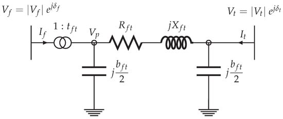
Figure 1.
Generic branch model (π-circuit) for modeling transmission lines ( & ), in-phase transformers () and phase-shifting transformers (). The transformer tap ratio is modeled only on the from-Bus side of the branch model.
From the π-circuit model, we can derive for each branch a branch admittance matrix , which relates the complex from-bus and to-bus current injections & , respectively, to the complex from-bus and to-bus voltages & , respectively, as follows:
with
The elements of the branch admittance matrices can be used to assemble the bus admittance matrix which describes the relation between the vector of complex bus current injections to the vector of complex bus voltages for the entire power network.
The steady state power balance in the power system is derived from Kirchhoff’s Current Law (KCL, i.e., all incoming and outgoing currents at a bus must sum up to zero) applied to each bus in the network, which yields the following complex power balance matrix equation for the entire network:
where the left hand side describes the active and reactive power injections/extractions at generation/load buses, respectively, and the right hand side the incoming and outgoing apparent power flows from transmission lines and transformers.
The operation of a power system is restricted by a number of constraints imposed by technical components and stakeholders (producers, consumers, regulators etc.) involved in the power supply chain. Transmission lines, for instance, can only transport a limited amount of power due to thermal restrictions, while the operation of power plants is limited by the capability curves of the installed generators. The power transmission system operator (TSO) is responsible for respecting these constraints, while operating the system in an economic and secure manner. The real time power dispatch in an electric power system can be described by a steady state AC-optimal power flow model (AC-OPF) [50], which is expressed by the following non-linear inequality constrained optimization model:
where the decision variables expressed by vector
are the set of bus voltage angles Δ, bus voltage magnitudes and active and reactive power generation and , respectively. Equation (5) is a scalar quadratic objective function, which describes the total operating costs for each committed generation unit in terms of its active power generation, while the non-linear equality constraints expressed by Equations (6)–(9) describe the set of active and reactive power balance equations derived from matrix Equation (4). Equations (10) and (11) are non-linear inequality constraints, which describe the transmission capacity limits for each line, while the upper and lower limits of the decision variables are described by Equations (13)–(15). For each isolated sub network one bus is chosen as the voltage angle reference (see Equation (12)), i.e., the voltage angle of the reference bus is set to zero.
The described AC-OPF model is implemented into the open source power flow library MATPOWER [51], which we utilize as the power system simulator in the context of the proposed simulation framework.
4.2. Gas System Model
Similar to the power system network, the gas network is described by a directed graph composed of nodes V and branches E. Facilities with an inlet, outlet and flow direction are modeled as branches, while connection points between these branches as well as entry and exit stations are represented by nodes. Branches, in turn, can be distinguished between active and passive branches. Active branches represent controlled facilities, which can change their state or control during simulation, such as compressor stations, regulator stations and valves, while passive branches, such as pipelines and resistors represent facilities or components whose state is fully described by the physical equations, derived from the conservation laws. A description of the different branch types is given in Table 1. Nodes can also be differentiated according to their function into supply, demand, storage and junctions. A description of the different node types and their corresponding node facilities is given in Table 2.

Table 1.
Basic elements comprising gas transport networks.
Table 2.
Classification and characteristics of nodes in the network.
The gas model proposed in this study includes sub-models of all important facilities comprising a gas transport system, such as pipelines, compressor stations (CS), production fields (PRO), cross-border import (CBI) and export stations (CBE), city gate stations (CGS), stations of direct served customers (GFPPs, IND), liquefied natural gas (LNG) regasification terminals and underground gas storage (UGS) facilities. The model is able to capture appropiately [52,53] the reaction of gas transport systems to load variations (i.e., daily and seasonal changes of gas demands at offtake points) and disruption events (e.g., loss of supply from an entry point, failure in a compressor station, etc.) with moderate computational cost, taking into account the physical laws governing the dynamic behavior of gas transport systems. The accuracy of the proposed gas model has been confirmed in [52,53], where it is benchmarked against a commercial software package. In the following we give a brief description of the physical equations used fro describing the gas system. We refer to previous publications, for more details on the gas model implemented in SAInt [52,53,54].
The dynamic behavior of a gas transport system is predominantly determined by the gas flow in pipelines. The set of non-linear hyperbolic partial differential equations (PDE) describing the transient flow of natural gas in pipelines are derived from the law of conservation of mass, momentum and energy and the real gas law.
Applying these laws on an infinitesimal control volume () of a general pipeline with a constant cross-sectional area A and an infinitesimal length (see Figure 2) and assuming the parameters describing the gas flow dynamics along the pipe coordinate x are averaged over A, yields the following set of fundamental Partial Differential Equations (PDEs) describing the gas flow through pipelines (the assumption of averaging the flow parameters over the cross-sectional area can be justified as long as the pipe length L is much greater than the pipe diameter D which is the case in transmission networks where is of order or lower):
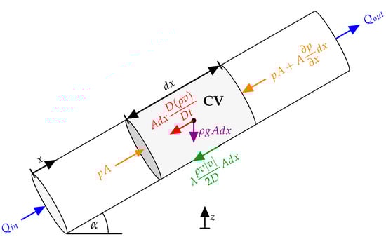
Figure 2.
Forces acting on a control volume in a general gas pipeline.
Law of Conservation of Mass—Continuity Equation:
Newton’s Second Law of Motion—Momentum Equation:
First Law of Thermodynamics - Energy Equation:
Real Gas Law - State Equation:
The fundamental equations are typically simplified by adapting them to the prevailing conditions in transport pipelines. The most common assumptions are isothermal flow (i.e., constant temperature in time and space, thus, energy equation is redundant and can be neglected) and small flow velocities (i.e., relatively small Mach numbers, thus, convective term in momentum equation is negligible compared to the other terms), which applied to the above equations yields the following set of non-linear hyperbolic PDEs:
with
The above PDEs express the physical behavior of the gas flow in each pipe section in the gas model. We can integrate the set of PDEs for the entire network into one coupled equation system by applying the following integral form of the continuity equation to a nodal control volume in the network, assuming all pipelines in the network are divided into a finite number of pipe segments:
with
Equation (23) can be expressed for each nodal control volume in the network, resulting in set of equations with unknown state variables, where and denote the number of nodes and branches, respectively. Thus, additional independent equations are required in order to close the entire problem. These equations are provided by the pressure drop equation for each pipe segment derived in Equation (22) and the equations describing the control modes and active constraints of non-pipe facilities [52]. The differential equations can be discretized using the following fully implicit finite difference approximations for the state variables p, Q and L and their time and space derivatives:
The resulting (non-)linear finite difference equations and control equations of non-pipe facilities are solved iteratively by a sequential linearisation method [55]. For more details on the equations describing the control and active constraints of non-pipe facilities and the algorithm for solving the gas model we refer to [52,53,54].
Furthermore, we use the following expression for computing the quantity of gas stored in each pipe section (line pack):
with
where is the mean pressure in the pipe section and, and are the inlet and outlet gas pressure, respectively. The ramping of a GFPP depends on the availability of line pack in the hydraulic area (sub network bounded by controlled facilities) the GFPP is connected to. We consider the availability of line pack by setting a minimum nodal gas pressure threshold for the corresponding GFPP node. Since line pack is linearly correlated to the mean gas pipeline pressure, GFPPs operate only if a specific line pack level equivalent to the specified minimum pressure is available.
The presented gas model is implemented into the simulation tool SAInt, which we use as a simulator for the gas model in the proposed simulation framework.
4.3. Interconnection between Gas and Power Systems
As discussed in the previous sections, gas and electric power systems are physically interconnected at different facilities. In this paper, we consider the most important connections between both systems as follows:
- Power supply to electric drivers installed in gas compressor stations:The electric power consumed by the compressor station can be described by the following expression (derived from the first and second law of thermodynamics for an isentropic compression process) describing the required driver power for compressing the gas flow Q from inlet pressure to outlet pressure [56,57]:where f is a factor describing the fraction of total driver power provided by electric drivers, the average adiabatic efficiency of the compressors, the average mechanical efficiency of the installed drivers, the outlet pressure, , , the inlet pressure, compressibility factor, temperature, respectively, R the gas constant, κ the isentropic exponent.The power supply of the gas network is added to the active power demand in the electric model.
- Electric power supply to LNG terminals and UGS facilities:We capture this interaction by assuming a generic linear function in terms of the regasification or withdrawal rate , respectively:
- Fuel gas offtake from gas pipelines for power generation in GFPPs:The required fuel gas for active power generation at plant i can be expressed in terms of the thermal efficiency of the GFPP and the gross calorific value of the fuel gas, as follows:
4.4. Integrated Simulation Framework for Security of Supply Analysis
The modeling framework carried out within SAInt considers the integrated gas and electricity transmission network under cascading outage contingency analysis. The cascading outages are investigated when the gas or electricity system has just experienced a disruption, like a shortage in supply or transmission capacity. The framework comprises of
- (i)
- a simulator (MATPOWER) for solving an AC-OPF for the power system,
- (ii)
- a transient hydraulic gas simulator (SAInt) for the gas system which includes sub-models of all relevant pipe and non-pipe facilities
- (iii)
- and an interface (SAInt) which handles the communication and data exchange between the two isolated simulators.
SAInt is composed of two separate modules, namely, SAInt-API (Application Programming Interface) and SAInt-GUI (Graphical User Interface). The API, is the main library of the software and contains the solvers, routines and classes for instantiating the different objects included in gas and electric systems. In order to perform power flow calculations and to extend the functionality of the software, the API has been linked to MATLAB using the Matlab COM Automation Server. This link has been used to establish a communication between the Matlab-based open source power flow library MATPOWER [51] and SAInt-API. This allows the execution of AC-Power Flow and AC-OPF with MATPOWER and the evaluation and visualization of the obtained results using SAInt-GUI [52]. For more information on SAInt we refer to previous publications [52,54].
The proposed simulation framework is illustrated in the flow diagram depicted in Figure 3, which is explained further below.
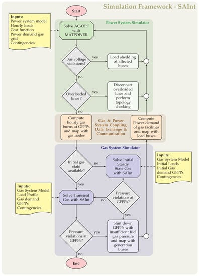
Figure 3.
Flow chart of the proposed Simulation Framework SAInt, showing the implemented algorithm.
The power model proposed in this paper is designed to provide a realistic representation of the behavior of an actual power system when subjected to contingencies. Cascading effects of contingencies in the power grid are very complex phenomenona, and identifying the typical mechanisms of cascading failures and understanding how these mechanisms interact during blackouts is an important research area [58,59,60,61,62,63]. Potential mechanisms that might be modeled include overloaded line tripping by impedance relays due to the low voltage and high current operating conditions, line tripping due to loss of synchronism, the undesirable generator tripping events by overexcitation protection, generator tripping due to abnormal voltage and frequency system condition, and under-frequency or under-voltage load shedding. For each additional mechanism of cascading failure included in a model, assumptions must be made about how the system will react to these rarely observed operating conditions.
This paper introduces a steady state AC-flow model which is adapted to reflect a set of corrective actions performed by TSOs when trying to return the system to a stable operating condition after a contingency.
While the initial contingency can usually be considered as being a random event, an interaction of cascading failure mechanisms exists in the subsequent events. For example, the loss of critical components such as tripping of transmission lines creates load redistribution to other components, which might become overloaded. The overall network is then weakened due to the stress on remaining elements, possibly leading to an instability. If corrective action plans are not applied quickly further failures might be created as a consequence leading to a blackout. In this paper, this cascading failure phase, starting with the initiating event is modeled, where the cascading contingencies occurrence are affected by operator actions and the times between subsequent events are considered in a range of tens of seconds to 1 h. Various system adjustments that are considered include the post-contingency redispatch of active and reactive resources, cascade tripping of an overloaded transmission line, tripping or re-dispatching of generators due to load/generation imbalance, and load shedding at load buses to prevent a complete system blackout when insufficient voltage magnitudes are observed.
The initial state of the model is obtained by solving the standard AC optimal power-flow problem as described in Equations (5)–(15), which yields the optimum hourly generator dispatch for given hourly loads, cost functions for each generator and bus voltage and line loading constraints. To execute this task MATPOWER 6.01b AC-OPF algorithm is applied [51].
Any change from the initial state caused by a contingency event, such as a (simultaneous) failure of one or more transmission lines, failure of a generation unit or decreased amount of generation capacity due to lack of gas supply, can be introduced in the model by defining a scenario event for the corresponding facility, which is composed of an event time, an event parameter and its corresponding value.
Whenever a contingency is observed in the system, an imbalance between total generation and total load may occur. In order to re-balance the system, the model redistributes the missing or excess power to the remaining facilities in the power grid. The power re-dispatch is obtained by running the AC-OPF model, while considering the new topology triggered by a previous disruption (e.g., lines and generation units may be disconnected). However, since the system is under a stressed state, the AC-OPF algorithm may deliver an infeasible solution, that does not satisfy the convergence criteria, since system constraints such as line overloading or voltage limits cannot sustain the desired system loads. In order to allow the system to find a converged solution, the bus voltage () and line capacity constraints ( & ) in the standard AC-OPF formulation are relaxed for the re-dispatching process. The re-dispatching process is followed by a two step feasibility checking procedure. In step one, bus voltage violations are mitigated by performing load shedding at the affected buses and recomputing the relaxed AC-OPF until no voltage violations are detected, so called under-voltage load shedding. The model assumes that there is enough time for the operator to implement under voltage load shedding to prevent a voltage collapse which is the root cause of most of the major power system disturbances [64,65,66]. The model sheds load in blocks of 2% for the corresponding bus until the relaxed bus voltage constraint is satisfied. If a violation is not eliminated although the load sheds more than 50% of its original load, we assume complete failure of the affected bus and set the load value to zero [8]. The second step of the feasibility checking procedure follows after all bus voltage violations have been remedied in the first step. During the re-dispatching process new failures may occur at certain components as they become overloaded. In this paper the overloads are aimed to be strictly avoided for all component contingencies. This means that it is assumed that the probability for line trip is 1 when line flow exceeds its thermal capacity with a tolerance parameter. The second step involves disconnecting overloaded transmission lines from the power grid and recomputing the relaxed AC-OPF until a feasible solution is obtained. It should be noted that, the connectivity of the network is checked in every simulation step prior to the AC-OPF computation in order to detect isolated facilities. The algorithm used for checking the connectivity is based on the well-known minimum spanning tree algorithm and is described in detail in [8].
After obtaining a feasible solution for the power system, the resulting hourly power generation of GFPPs is converted into a hourly gas demand profiles and provided as input to the gas model. The gas model needs an initial state for running the transient simulation. This state can either be a solution of a steady state simulation or the terminal state of a transient simulation. If an initial state is not available the algorithm uses the initial loads of the generated gas demand profiles for GFPPs to compute a steady state solution. This solution is then used as an initial state for the transient simulation. After each transient or steady state simulation the algorithm checks if the fuel gas pressures at GFPP nodes are sufficient to operate the facilities. If an insufficient fuel gas pressure is detected, the affected GFPP is shut-down and the power system model is recomputed. The algorithm is terminated if no pressure violations are detected after the transient gas simulation. Finally, the amount of energy not supplied is calculated as an indicator of the impact of the disruption event.
The gas and electric model described above are connected through an interface which enables the communication and data exchange between the two simulators (i.e., MATPOWER as power system simulator and SAInt as transient gas simulator, see Figure 3). The time integration of the combined model is performed separately for both systems and the interconnection between both systems is established through data exchange at discrete time and space points.
The timing of the power model is based on the discrete event simulation concept. It is assumed that the configuration of the power system (e.g., the state of generation units and lines) remains unchanged between events and changes only at the time of the specific event. If no events are scheduled or triggered in the course of the simulation the time step of the power system corresponds to a reference time step of 1 hour.
In contrast to the power system, the time integration of the transient gas model, is based on a dynamic time step adaptation method (DTA), which adapts the time resolution with respect to the control changes of controlled gas facilities during the solution process. The DTA allows capturing rapid changes in the gas system (shut-down of a power plant or compressor station etc.) with a higher time resolution. In this context, the gas model can be viewed as a quasi-continuous system, where the values of the state variables (i.e., nodal pressure p, element flows Q and nodal loads L) between two discrete time points are approximated by linear interpolation. If no events are scheduled or triggered in the course of the simulation the time step of the gas system corresponds to a reference time step of 15 min.
The gas and power system simulator used in the simulation framework have both been tested and verified. The gas simulator SAInt was benchmarked against a commercial software in previous publications [52,53] and the power system simulator MATPOWER [51] is well known and accepted by the scientific community.
In the following section, the proposed framework is applied to perform a contingency analysis for an integrated gas and power system network.
5. Model Application
In this section, an integrated gas and power network is constructed to demonstrate the previously discussed simulation framework implemented in SAInt. Three supply side scenarios (one non-disrupted scenario (base case) and two supply disruption scenarios) are presented in order to demonstrate the value of the proposed framework and to stress the importance of modeling the interdependence between gas and power systems with respect to security of supply.
The proposed scenarios are performed on the test network depicted in Figure 4. (The test network applied in this paper is a model of a real gas and electric power network of an European region. Due to confidentiality reasons and the sensitivity of the presented results, the topology and facility names of the real network have been disguised. The network topology and properties used for the computations, however, are realistic data for the combined network). The scenarios are composed of a number of extreme events causing more than two network facilities to be deactivated or to cascade out of service.
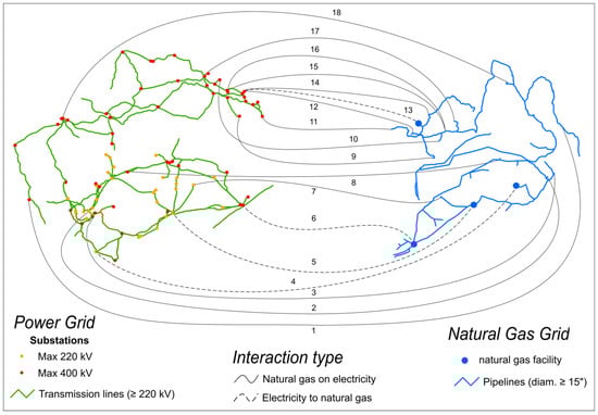
Figure 4.
Integrated gas and power network applied in the case study. Map shows a real network of an European region, which has been disguised due to confidentiality reasons. The network data and properties used for the case studies, however, are original input data for the actual network. The solid black lines (lines 1–3, 7–12, 14–18) represent interconnections between Gas Fired Power Plants (GFPPs) in the power grid (left) and their fuel gas offtake points in the gas grid (right), while the dashed black lines (4–6, 13) represent interconnections between electric buses in the power grid (left) supplying electric power to connected facilities in the gas grid.
The sample network includes a power grid with 158 buses, 62 generating units with 22,076 ( MW) installed capacity based on different generation mix that mainly consists of lignite (33%), natural gas (28%), coal (20%), wind power (7%) and others (12%). The transmission system consists of 194 high voltage transmission lines with total line length of approx. 8000 (km). The base voltage levels for the transmission lines are distinguished between 200 (kV) and 400 (kV).
The solution of the AC-OPF equations requires the knowledge of the voltage levels, admittances as well as the maximum thermal capacities of the transmission lines. The reactance of a line depends mainly on its physical properties. It increases proportionally to the geometric length of the line. Therefore, in the scope of this work, we assume equal physical properties for all lines and use the length to determine the reactance. A typical value for the reactance of a transmission line per unit length is 0.2 (Ω/km). Regarding the thermal capacities of the transmission lines, we assume a transmission capacity of 800 (MW) for 400 (kV) lines and 530 (MW) for 200 (kV) lines. In AC-OPF analysis the reactive power has strong influence on voltage drop thresholds. Thus, during AC OPF analysis, the maximum and minimum voltage levels for buses are considered and a value between 1.12 and 0.96 (p.u.) is assigned, respectively.
The gas network, comprises of 345 pipe segments with a total pipe length of roughly 4000 (km), 10 compressor stations and 352 nodes (54 exit stations to the local distribution system (CGS), 15 stations to direct served customers (14 GFPPs and one large industrial customer (IND)), two cross border export stations (CBE_1 & CBE_2), one cross border import station (CBI), one LNG terminal (LNG), one production field (PRO) and one underground gas storage facility (UGS). The CBI, PRO, LNG terminal and UGS facility are pressure controlled, while each compressor station is pressure ratio controlled with a pressure ratio set point ranging between 1.02 and 1.2. The input data for the compressor stations are listed in Table 3. The data used for the facilities supplying gas to the gas system are given in Table 4, while the data for the GFPPs are listed in Table 5. The minimum delivery pressure for the 14 GFPPs is set to 30 (bar-g) while the time needed to reach complete shut-down of a GFPP is set to 45 (min).
Table 3.
Compressor station control (PRSET—Pressure Ratio Set Point) and constraints (PRMAX— Maximum Pressure Ratio, PWMAX—Maximum Available Driver Power, POMAX—Maximum Discharge Pressure, PIMIN—Minimum Suction Pressure).
Table 4.
Input data for facilities supplying the gas system with gas.
Table 5.
Input data for GFPPs connected to the gas and electric power system. Numbering of GFPPs corresponds to the numbering of the solid interconnection lines in Figure 4.
The transient scenarios for the integrated gas and power network are simulated by assigning the relative load profile depicted in Figure 5 to the relevant exit stations (left plot represents the gas load profile and right plot the power load profile). It should be noted that, the relative load profile for the gas system is only assigned to CGSs, which are the connection points between the gas transmission and local distribution system. For all other exit stations (CBE_1, CBE_2, IND) a constant load profile corresponding to the steady state load is assumed. The absolute values of the load profile for CGS nodes are obtained by multiplying the steady state load with the relative values in Figure 5 (left plot). The load profiles of the 14 GFPPs in the gas model are provided by the power model based on allocating the results obtained from the AC-OPF analysis to the corresponding nodes in the gas model. For the power network, the resulting loads for a time window of 24 h are obtained by multiplying the initial loads by the relative profile depicted in Figure 5 (right plot).
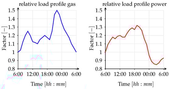
Figure 5.
Load profiles gas (left side) and power (right side) networks.
All 14 GFPPs in the power grid are physically interconnected to the gas network. Furthermore, we assume additional interconnections between the gas and power network at two compressor stations, at the LNG terminal and at the UGS facility, which are supplied with power from the electric grid. The integrated gas and power network with 18 physically interconnected facilities is illustrated in Figure 4. Additional input parameters for the gas simulator are given in Table 6.
Table 6.
Input data for the gas simulator.
Applying the simulation tool SAInt on the presented sample network, some preliminary observations on cascading outage contingency analysis can be made. Initially, a base case scenario (scenario 0) with no supply disruption in any of the two interlinked networks is introduced. In the base case scenario, we capture the behavior of the networks at normal operation. Then, we compare the base case scenario with two scenarios, where we introduce a number of disruption events and simulate the reaction of the system to these events. The simulated grid is generated with a time resolution of 900 (s) and all scenarios are simulated for one gas day from 06:00 to 06:00 (For the case study, we chose a simulation time of one operating day (24 h) with a time resolution of 15 min for the gas model and a time resolution of one hour for the power model, in order to keep the size of input data and information at a moderate level for the results discussion. However, the framework is designed to allow an extension and adaptation of the time window and resolution depending on if a short or long term study of a contingency scenario is of interest.) It should be noted that although it is possible to change the status of the failed components (repairing and restoration can be modeled) within the simulation, the scenarios that are presented in this study do not take into account the repairing activity in order to analyze system capabilities in worst-cases.
While the first scenario involves a disruption of several supply points in the gas network, the second scenario includes supply disruptions triggered by the power network. In scenario 1, we assume a reduced regasification rate for the LNG terminal from maximum via a ramp-down between 06:00 and 07:00 (see Figure 6), which corresponds to an expected 7-day delay in cargo. In addition, we assume a supply disruption at the production field causing a ramp down of the supply between 08:00 and 9:00 (see Figure 6). Furthermore, a 30% supply reduction at CBI station at time 14:00 is implemented via a ramp-down between 14:00 and 15:00 (see Figure 6). Scenario 2 is related to power network contingencies and initial contingency set consist of the loss of major lignite power plant with 1157 (MW) operational capacity at 07:00 and 70% lack of power generation from wind turbines at 06:00 (see Figure 6).
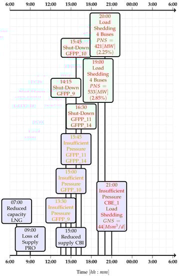
Figure 6.
Timing of initial (black) and cascading (orange, red) events for Scenario 1. Abbreviation PNS stands for power not supplied, while GNS stands for gas not supplied, value in brackets refers to the fraction of not supplied power/gas with respect to total power/gas loads.
In the following, we discuss the simulation results for the three scenarios (The simulation results and conclusions are based on the input data chosen for the sample network. While some data were provided by the TSOs, others were not available (e.g., pipe roughness, gas temperature, line properties etc.) and were therefore estimated using typical values. Thus, these input data are connected with uncertainties).
The sequence of initial events (shown in black) and their consequences (shown in orange and red) are summarized in Figure 6 and Figure 7 for scenario 1 and scenario 2, respectively. It can be seen from the figures, that when a minimum pressure violation for a GFPP is detected in the gas model, the failure of the corresponding power plant is applied after 45 (min) due to the required shut-down time. Figure 8, Figure 9 and Figure 10 show the difference in gas supply to the system through the CBI station, the production field and the LNG terminal. There is a big difference in inflows to the system through these supply points in scenario 0 and scenario 1, where the difference is more than 20 (Msm3/d) (Million standard cubic meter per day, where the reference pressure is 1.0135 (bar) and the reference temperature is 0 (°C)). The impact of this observation can be seen in Figure 8, Figure 9, Figure 10, Figure 11 and Figure 12. Figure 11 shows that the disruptions introduced in scenario 1 have the highest impact on the gas network, since the flow balance, which is the sum of inflow minus sum of outflow, is always negative; the system is not able to supply enough gas to balance the demand. In fact, the flow balance is quite negative throughout the time, peaking down to equivalent daily flows of (Msm3/d). As a result, the quantity of gas stored in the pipeline (i.e., the line pack) reduces significantly as time passes. The flow balance can be viewed as the time derivative of the line pack, thus, if the flow balance is negative the line pack decreases and if positive the line pack increases. A zero flow balance corresponds to no change in line pack. Latter is the assumption made in steady state gas models, which cannot capture the changes in line pack, and therefore, the real behavior of the gas system appropriately. Moreover, Figure 11 shows a decrease in line pack from ca. 85 to 67 (Msm3/d) for scenario 1 (approx. 18 (Msm3/d) lost along the day in the pipelines). In contrast, in scenario 0 only approx. 1.5 (Msm3/d) of line pack is extracted.
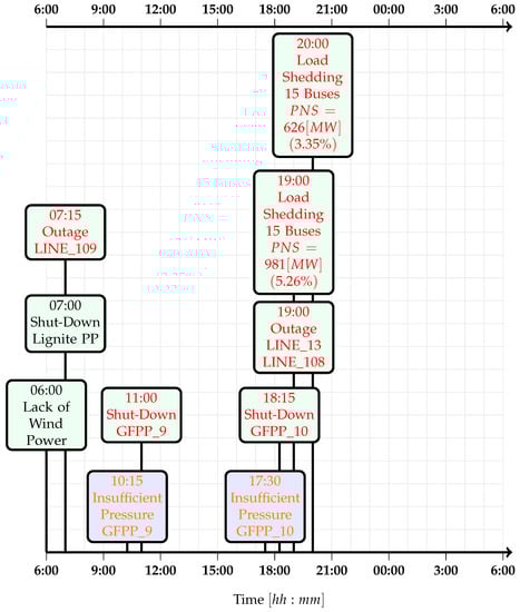
Figure 7.
Timing of initial (black) and cascading (orange, red) events for Scenario 2. Abbreviation PNS stands for power not supplied, value in brackets refers to the fraction of not supplied power with respect to total loads.
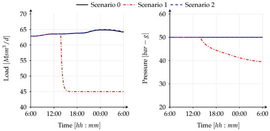
Figure 8.
Time evolution of gas supply and pressure at the cross border import (CBI) node for the computed scenarios.
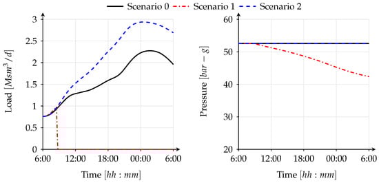
Figure 9.
Time evolution of gas supply and pressure at the production field for the computed scenarios.
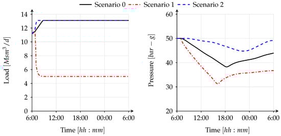
Figure 10.
Time evolution of regasification rate and pressure at the liquefied natural gas (LNG) terminal for the computed scenarios.
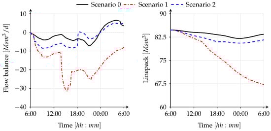
Figure 11.
Time evolution of flow balance (sum of inflow minus sum of outflow) and line pack for the computed scenarios.
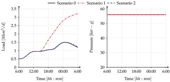
Figure 12.
Time evolution of withdrawal rate and pressure at underground gas storage (UGS) facility for the computed scenarios.
This produces a steady decrease of pressure in the CBI station, the production field and the LNG facility causing the pressure to reduce to approx. 39, 42 and 31 (bar-g), respectively (see Figure 8, Figure 9 and Figure 10).
An important observation is the pressure drop to approximately 31 (bar-g) at the LNG terminal, which is the main gas supplier for some of the GFPPs in the hydraulic region. This value is slightly above the 30 (bar-g) minimum delivery pressure threshold required by the GFPPs. When gas supplies are scarce, the only way to keep maintain sufficient pressure and to allow the network to continue operating is to reduce consumption, either through curtailment or fuel switching, if there is the chance to do this with some power plants. In scenario 1, gas curtailment at GFPPs is implemented, presuming that replacement fuel is not available in any of the investigated GFPPs.
Figure 12 shows the behavior of the UGS facility, the only supply node able to increase gas supply to satisfy the increased demand in scenario 1. The UGS facility is able to maintain its pressure set point till the end of the simulation (see Figure 12). The disconnection of four GFPPs from the gas network at 14:15, 15:45 and 16:30, respectively, allows the gas system to continue running (see Figure 6 and Figure 13). The pressure and load profiles for failed GFPPs are given in Figure 13 and Figure 14. This curtailment was sufficient to cope with the pressure drop in the network. Therefore, there was no need of gas curtailment at CGSs, where protected customers (e.g., households, public services) are supplied with gas.
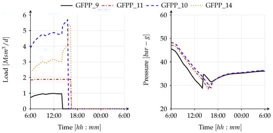
Figure 13.
Time evolution of load and pressure of failed GFPPs in scenario 1.
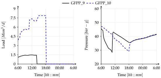
Figure 14.
Time evolution of load and pressure of failed GFPPs in scenario 2.
Figure 15 and Figure 16 depicts the voltage profiles for a selected number of buses, where minimum voltage violation is detected for scenario 1 and 2, respectively. In order to keep the bus voltage above the minimum voltage level, load shedding is implemented at the affected buses. The left plots in Figure 15 and Figure 16 show the voltage profiles of the affected buses for the computation where voltage violations were detected and no countermeasures were employed to avoid this violation, while the right plots show the voltage profiles after implementing load shedding at the affected buses. As can be seen in the right plots of Figure 15 and Figure 16, the bus voltages recover to a value above the minimum voltage threshold after load shedding is implemented. However, due to load shedding some customers connected to the affected buses are not supplied with enough electricity (see Figure 6 and Figure 7).
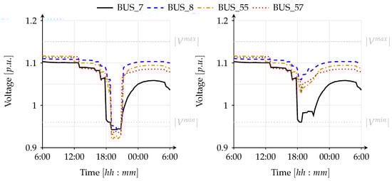
Figure 15.
Time evolution of bus voltage before load shedding (left) and after (right) for scenario 1. All four buses where load shedding was applied are shown in this figure.
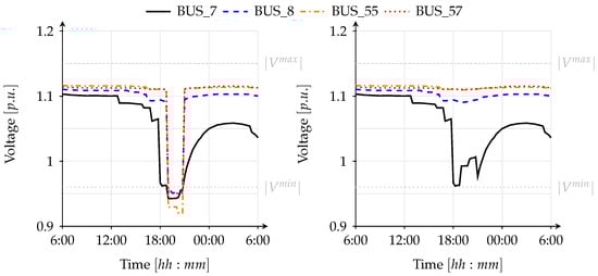
Figure 16.
Time evolution of bus voltages before load shedding (left) and after (right) for scenario 2. Load shedding was applied at 15 buses. Among these buses are the 4 buses from scenario 1, which are shown in this figure.
Regarding the CBE_1 station, due to the pressure drop at the station (see Figure 17), the flow is restricted around 21:00 because the threshold pressure of 30 (bar-g) is reached. This is the only way to keep minimum delivery pressure at that exit point; otherwise problems would arise downstream due to too low pressure. Figure 17, shows the drop in flow (around 8 (Msm3/d) ) at CBE_1 station due to the pressure restriction.
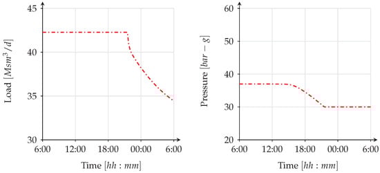
Figure 17.
Load and pressure profile of CBE_1 for scenario 1.
Moreover, the difference between scenario 0 and scenario 2 shows the gas system reaction to the electric side disruption. In Figure 11, it can be seen that the flow balance of the gas network in scenario 2 is more negative (the gas system loses more gas) than in scenario 0 until 18:00. This is caused by the increase in gas demand of GFPPs due to the disruption of the lignite power plant and the loss of power generation from wind turbines. The increase in gas demand of GFPPs leads to a pressure drop in two GFPPs, followed by the disconnection of the power plants from the network (see Figure 7 and Figure 14). The pressure and load profiles for failed GFPPs are given in Figure 14. The disconnection of the generators affects the loading of the gas system in a positive way. Moreover, the line pack starts to recover after 18:00 (see Figure 11).
The scenario results indicate clearly that the disruptions taking place in the gas network that affect GFPPs also affected the operability of the power network. After failure of each GFPP, the power model calculates the new generating profiles for all power plants and sends these profiles to the gas model. In scenario 1, the closure of 4 GFPPs due to low pressure levels in the gas system caused voltage violations in the electricity network at peak demand hour (19:00–20:00) because of the high amount of power transmission from relatively distant generators in order to compensate the missing generating capacity. This violation in voltage levels caused 954 (MW) of load shedding during 2 h (see Figure 6 and Figure 15). In scenario 2, the cascading effects are more severe including three line overloads and load shedding of 1607 (MW) at the peak demand hours (19:00–20:00, see Figure 7 and Figure 16). The initial failure of large capacity lignite power plant together with lack of power generation from wind power caused an increase in power generation from GFPPs. This increase results in pressure drops at two GFPPs followed by the closure of both facilities. The system has to implement these cascading effects in order to avoid a complete blackout in the overall network.
Furthermore, the results show that the impact of disruptions introduced in both scenarios is much higher for the power system than for the gas system Section 3.
6. Conclusions
In this paper, we developed an integrated simulation framework for cascading outage contingency analysis in combined gas and power system networks and demonstrated the capabilities of the implemented framework by applying it to a realistic, combined electricity and gas transmissions network of an European region.
The simulation framework is composed of a transient hydraulic model for the gas system and a steady state AC-OPF model for the power system. Both models, are derived from the physical laws governing the flow of gas and electrical power, respectively. Moreover, the most important facilities and their technical constraints are considered. The gas and power system models a coupled through coupling equations describing the fuel gas offtake of GFPPs for power generation and the power supply to LNG terminals, UGS facilities and electric driven compressor stations.
The model application was divided into three scenarios, namely, scenario 0 with no disruption, scenario 1 with gas side disruptions and scenario 2 with power side disruptions. The results of these scenarios show how disruption events triggered in one system propagate to the other system. In scenario 1, for instance, three major gas supply stations are disrupted and as a result a number of GFPPs are shut-down due to insufficient fuel gas pressure. This contingency propagates further to other buses in the power system, where load shedding is implemented in order to maintain the voltage levels above the minimum voltage threshold. Similar observations are made in scenario 2, where a drastic reduction in renewable energy generation together with a shutdown of a large power plant triggered a large increase in gas demand of GFPPs, leading to a rapid pressure drop in the gas network and the subsequent shut-down of GFPPs. Eventually, this circumstance increased the stress on the power system leading to minimum bus voltage violations in a couple of buses, which is remedied by applying load shedding at the affected buses.
Based on these key findings, it can be concluded that there is a need for close collaboration and coordination between gas and power TSOs. Data concerning pressures, flows, voltages etc., efficiently handled and communicated may introduce resilience on the integrated network. This has to be done via well-structured protocols that inform the other TSO about the grace periods and support that each network may grant the other. The use of models like the one proposed in this study may be of much help for getting part of this information to share with the other operator.
We believe it is fair to state that the integrated model allows for detailed fingerprinting and exploration of the effects of disruption in gas and/or power, to a level of detail that is not possible by qualitative, expert analysis. Once the data characterizing a gas and electricity grid have been loaded, experts can perform in-silico experiments at will to investigate the system, determine weak elements, and propose mitigation strategies. In both two scenarios, GFPP_9 and GFPP_10 fail, which merits an investigation into their position in the system. If in more scenarios it is these two plants that fail first, it could be decided to equip these with alternative backup fuel options. In the future, we intend to further develop the simulation framework to implement more simulation options and functionalities into the simulation tool SAInt in order to investigate the effectiveness of different demand and supply side measures to mitigate the consequences of supply disruptions in coupled gas and electric power systems.
Acknowledgments
This work has been developed within the framework of the European Program for Critical Infrastructure Protection (EPCIP) of the European Commission. We express our gratitude to our colleague Nicola Zaccarelli from the Joint Research Centre—Institute for Energy and Transport, in Petten, Netherlands, for providing the GIS-Data for the presented gas and electric model. We would also like to thank Tom van der Hoeven for the productive discussions and suggestions, which have improved the simulation tool SAInt.
Author Contributions
Kwabena Addo Pambour developed the simulation software SAInt, designed and implemented the simulation framework into SAInt and wrote the paper; Burcin Cakir-Erdener designed the simulation framework and the case studies, performed the computations, analyzed the results, and wrote the paper; Ricardo Bolado-Lavin reviewed the paper and proposed modifications to improve the design of the simulation framework and the case studies; Gerard P. J. Dijkema reviewed the paper and suggested changes to improve the quality of the paper.
Conflicts of Interest
The authors declare no conflict of interest.
Abbreviations
The following abbreviations are used in this manuscript:
| Abbreviations | |
| AC | Alternating current |
| API | Application Programming Interface |
| EU | European Union |
| ED | Economic dispatch |
| CBE | Cross Border Export |
| CBI | Cross Border Import |
| CBP | Cross Border Point |
| CEI | Critical Energy Infrastructures |
| CGS | City Gate Station |
| DC | Direct current |
| DTA | Dynamic Time Step Adaptation |
| GB | Great Britain |
| GFPP | Gas Fired Power Plant |
| GNS | Gas not supplied |
| GUI | Graphical User Interface |
| IND | Large Industrial Customer |
| KCL | Kirchoff’s Current Law |
| LNG | Liquefied Natural Gas |
| NGTS | National Gas Transport System |
| P2G | Power to Gas |
| PF | Power Flow |
| PDE | Partial Differential |
| PNS | Power not supplied |
| PRO | Production Fields |
| OPF | Optimal Power Flow |
| SAInt | Scenario Analysis Interface |
| SCUC | Security Constraint Unit commitment |
| SNG | Synthetic Natural Gas |
| TSO | Transmission System Operator |
| UC | Unit commitment |
| UGS | Underground Gas Storage |
| Mathematical Symbols | |
| A | cross-sectional area |
| a | transformer tap ratio |
| elements of the node-branch incidence matrix | |
| b | line charging susceptance |
| coefficients of cost function | |
| c | speed of sound |
| control volume | |
| D | inner pipe diameter |
| e | Euler’s number |
| E | set of branches |
| f | electric driver factor |
| g | gravitational acceleration |
| G | directed graph |
| gross calorific value | |
| electric curent injection at from bus | |
| electric curent injection at to bus | |
| j | imaginary number |
| coefficients of coupling equation | |
| L | nodal load |
| fuel gas offtake for power generation at GFPPs | |
| l | pipe length |
| line pack | |
| M | number of pipe section |
| n | simulation time point |
| number of gas nodes | |
| number of buses, number of branches | |
| number of compressor stations | |
| number of power generation units | |
| number of GFPPs | |
| number of inequality constraints | |
| number of transmission lines and transformers | |
| active power demand | |
| power demand of compressor stations | |
| power demand of LNG terminals and UGS facilities | |
| active power generation | |
| vector of active power generation | |
| p | gas pressure (vector) |
| inlet pressure | |
| outlet pressure | |
| mean pipe pressure | |
| Q | gas flow rate, reactive power |
| vector of reactive power generation | |
| R | gas constant, line resistance |
| apparent power injection at from bus of branch k | |
| maximum transmission capacity of branch k | |
| apparent power injection at to bus of branch k | |
| vector of apparent power flow | |
| t | time, complex transformer tap |
| time point | |
| time step | |
| T | temperature |
| reference temperature | |
| v | gas velocity |
| V | complex bus voltage, set of nodes |
| vector of complex bus voltage | |
| vector of complex bus voltage magnitudes | |
| bus voltage magnitude | |
| nodal volume | |
| X | line reactance |
| x | pipeline coordinate |
| vector of decision variables | |
| pipe segment length | |
| Y | line admittance |
| branch admittance matrix | |
| bus admittance matrix | |
| Z | compressibility factor, impedance |
| Greek Symbols | |
| α | inclination |
| coefficients of heat rate curve | |
| δ | voltage angle |
| Δ | vector of bus voltage angles |
| ϵ | residual tolerance |
| compressor adiabatic efficiency | |
| driver efficiency | |
| thermal efficiency | |
| κ | isentropic exponent |
| λ | friction factor |
| transformer phase shift angle | |
| ρ | gas density |
| gas density at reference conditions | |
| Physical Units | |
| (bar-g) | bar gauge (absolute pressure minus atmospheric pressure) |
| (p.u.) | per unit |
| (Msm3) | millions of standard cubic meters (line pack, inventory) |
| (Msm3/d) | millions of standard cubic meters per day (gas flow rate) |
| (sm3) | standard cubic meters (line pack, inventory) |
References
- North American Electric Reliability Corporation (NERC). Accommodating an Increased Dependence on Natural Gas for Electric Power, Phase II: A Vulnerability and Scenario Assessment for the North American Bulk Power; Technical Report; North American Electric Reliability Corporation (NERC): Atlanta, GA, USA, 2013. [Google Scholar]
- Pearson, I.; Zeniewski, P.; Gracceva, F.; Zastera, P.; McGlade, C.; Sorrell, S. Unconventional Gas: Potential Energy Market Impacts in the European Union; Technical Report; JRC Scientific and Policy Reports EUR 25305 EN; Joint Research Centre of the European Commission: Petten, The Netherlands, 2012. [Google Scholar]
- Judson, N. Interdependence of the Electricity Generation System and the Natural Gas System and Implications for Energy Security; Technical Report; Massachusetts Institute of Technology Lincoln Laboratory: Lexington, MA, USA, 2013. [Google Scholar]
- Clegg, S.; Mancarella, P. Integrated modeling and assessment of the operational impact of power-to-gas (P2G) on electrical and gas transmission networks. IEEE Trans. Sustain. Energy 2015, 6, 1234–1244. [Google Scholar] [CrossRef]
- Acha, S. Impacts of Embedded Technologies on Optimal Operation of Energy Service Networks. Ph.D. Thesis, University of London, London, UK, 2010. [Google Scholar]
- Rubio Barros, R.; Ojeda-Esteybar, D.; Ano, A.; Vargas, A. Integrated natural gas and electricity market: A survey of the state of the art in operation planning and market issues. In Proceedings of the Transmission and Distribution Conference and Exposition: Latin America 2008 IEEE/PES, Bogota, Colombia, 13–15 August 2008.
- Rubio Barros, R.; Ojeda-Esteybar, D.; Ano, A.; Vargas, A. Combined operational planning of natural gas and electric power systems: State of the art. In Natural Gas; Potocnik, P., Ed.; INTECH Open Access Publisher: Rijeka, Croatia, 2010. [Google Scholar]
- Cakir Erdener, B.; Pambour, K.A.; Lavin, R.B.; Dengiz, B. An integrated simulation model for analysing electricity and gas systems. Int. J. Electr. Power Energy Syst. 2014, 61, 410–420. [Google Scholar] [CrossRef]
- Abrell, J.; Weigt, H. Combining Energy Networks; Electricity Markets Working Papers WP-EM-38 2010; TU Dresden: Dresden, Germany, 2010. [Google Scholar]
- Özdemir, O.; Veum, K.; Joode, J.; Migliavacca, G.; Grassi, A.; Zani, A. The impact of large-scale renewable integration on Europe’s energy corridors. In Proceedings of the IEEE Trondheim PowerTech, Trondheim, Norway, 19–23 June 2011; pp. 1–8.
- Möst, D.; Perlwitz, H. Prospect of gas supply until 2020 in Europe and its relevance of the power sector in the context of emissions trading. Energy 2008, 34, 1510–1522. [Google Scholar] [CrossRef]
- Lienert, M.; Lochner, S. The importance of market interdependencies in modelling energy systems—The case of European electricity generation market. Int. J. Electr. Power Energy Syst. 2012, 34, 99–113. [Google Scholar] [CrossRef]
- Chen, H.; Baldick, R. Optimizing short-term natural gas supply portfolio for electric utility companies. IEEE Trans. Power Syst. 2007, 22, 232–239. [Google Scholar] [CrossRef]
- Asif, U.; Jirutitijaroen, P. An optimization model for risk management in natural gas supply and energy portfolio of a generation company. In Proceedings of TENCON 2009—2009 IEEE Region 10 Conference, Singapore, 23–26 January 2009.
- Kittithreerapronchai, O.; Jirutitijaroen, P.; Kim, S.; Prina, J. Optimizing natural gas supply and energy portfolios of a generation company. In Proceedings of PMAPS 2010—IEEE 11th International Conference on Probabilistic Methods Applied to Power Systems, Singapore, 14–17 June 2010; pp. 231–237.
- Duenas, P.; Barquin, J.; Reneses, J. Strategic management of multi-year natural gas contracts in electricity markets. IEEE Trans. Power Syst. 2012, 27, 771–779. [Google Scholar] [CrossRef]
- Spiecker, S. Analyzing market power in a multistage and multiarea electricity and natural gas system. In Proceedings of EEM—8th IEEE International Conference on the European Energy Market, Zagreb, Croatia, 25–27 May 2011; pp. 313–320.
- Weigt, H.; Abrell, J. Investments in a combined energy network model: Substitution between natural gas and electricity. In Proceedings of the Annual Conference 2014 (Hamburg): Evidence-Based Economic Policy, Hamburg, Germany, 7–10 September 2014.
- Gil, M.; Dueñas, P.; Reneses, J. Electricity and natural gas interdependency: Comparison of two methodologies for coupling large market models within the European regulatory framework. IEEE Trans. Power Syst. 2016, 31, 361–369. [Google Scholar] [CrossRef]
- Shahidehpour, M.; Fu, Y.; Wiedman, T. Impact of natural gas infrastructure on electricity power system security. IEEE Proc. 2005, 93, 1042–1056. [Google Scholar] [CrossRef]
- Li, T.; Eremia, M.; Shahidehpour, M. Interdependency of natural gas network and power system security. IEEE Trans. Power Syst. 2008, 23, 1817–1824. [Google Scholar] [CrossRef]
- Liu, C.; Shahidehpour, M.; Fu, Y.; Li, Z. Security-constrained unit commitment with natural gas transmission constraints. IEEE Trans. Power Syst. 2009, 24, 1523–1536. [Google Scholar]
- Li, G.; Zhang, R.; Chen, H.; Jiang, T.; Jia, H.; Mu, Y.; Jin, X. Security-constrained economic dispatch for integrated natural gas and electricity systems. Energy Procedia 2016, 88, 330–335. [Google Scholar] [CrossRef]
- An, S.; Li, Q.; Gedra, T. Natural gas and electricity optimal power flow. IEEE Transm. Distrib. Conf. Expo. 2003, 1, 138–143. [Google Scholar]
- Unsihuay, C.; Marangon Lima, J.; Zambroni de Souza, A. Modelling the integrated natural gas and electricity optimal power flow. In Proceedings of IEEE Power Engineering Society General Meeting, Tampa, FL, USA, 24–28 June 2007.
- Martínez-Mares, A.; Fuerte-Esquivel, C. Integrated energy flow analysis in natural gas and electricity coupled systems. In Proceedings of IEEE NAPS—North American Power Symposium, Boston, MA, USA, 4–6 August 2011; pp. 1–7.
- Liu, C.; Shahidehpour, M.; Wang, J. Coordinated scheduling of electricity and natural gas infrastructures with a transient model for natural gas flow. Chaos Interdiscip. J. Nonlinear Sci. 2011, 21. [Google Scholar] [CrossRef] [PubMed]
- Chaudry, M.; Jenkins, N.; Strbac, G. Multi-time periode combined gas and electricity network optimisation. Electr. Power Syst. Res. 2008, 78, 1265–1279. [Google Scholar] [CrossRef]
- Clegg, S.; Mancarella, P. Integrated electrical and gas network modelling for assessment of different power-and-heat options. In Proceedings of the Power Systems Computation Conference (PSCC), Wroclaw, Poland, 18–22 August 2014; pp. 1–7.
- Qadrdan, M.; Chaudry, M.; Wu, J.; Jenkins, N.; Ekanayake, J. Impact of a large penetration of wind generation on the GB gas network. Energy Policy 2010, 38, 5684–5695. [Google Scholar] [CrossRef]
- Qadrdan, M.; Jenkins, N.; Ekanayake, J. Operating strategies for a GB integrated gas and electricity network considering the uncertainty in wind power forecasts. IEEE Trans. Sustain. Energy 2014, 5, 128–138. [Google Scholar] [CrossRef]
- Chertkov, M.; Backhaus, S.; Lebedev, V. Cascading of fluctuations in interdependent energy infrastructures: Gas-grid coupling. Appl. Energy 2015, 160, 541–551. [Google Scholar] [CrossRef]
- Alabdulwahab, A.; Abusorrah, A.; Zhang, X.; Shahidehpour, M. Coordination of Interdependent Natural Gas and Electricity Infrastructures for firming the variability of wind energy in stochastic day-ahead scheduling. IEEE Trans. Sustain. Energy 2015, 6, 606–615. [Google Scholar] [CrossRef]
- Cui, H.; Li, F.; Hu, Q.; Bai, L.; Fang, X. Day-ahead coordinated operation of utility-scale electricity and natural gas networks considering demand response based virtual power plants. Appl. Energy 2016, 176, 183–195. [Google Scholar] [CrossRef]
- Bai, L.; Li, F.; Cui, H.; Jiang, T.; Sun, H.; Zhu, J. Interval optimization based operating strategy for gas-electricity integrated energy systems considering demand response and wind uncertainty. Appl. Energy 2016, 167, 270–279. [Google Scholar] [CrossRef]
- Zhang, X.; Shahidehpour, M.; Alabdulwahab, A.; Abusorrah, A. Hourly electricity demand response in the stochastic day-ahead scheduling of coordinated electricity and Natural Gas Networks. IEEE Trans. Power Syst. 2016, 31, 592–601. [Google Scholar] [CrossRef]
- Qadrdan, M.; Cheng, M.; Wu, J.; Jenkins, N. Benefits of demand-side response in combined gas and electricity networks. Appl. Energy 2016. [Google Scholar] [CrossRef]
- Saldarriaga, C.A.; Hincapié, R.A.; Salazar, H. A holistic approach for planning natural gas and electricity distribution networks. IEEE Trans. Power Syst. 2013, 28, 4052–4063. [Google Scholar] [CrossRef]
- Chaudry, M.; Jenkins, N.; Qadrdan, M.; Wu, J. Combined gas and electricity network expansion planning. Appl. Energy 2014, 113, 1171–1187. [Google Scholar] [CrossRef]
- Qadrdan, M.; Abeysekera, M.; Chaudry, M.; Wu, J.; Jenkins, N. Role of power-to-gas in an integrated gas and electricity system in Great Britain. Int. J. Hydrogen Energy 2015, 40, 5763–5775. [Google Scholar] [CrossRef]
- Clegg, S.; Mancarella, P. Storing renewables in the gas network: Modelling of power-to-gas seasonal storage flexibility in low-carbon power systems. IET Gener. Transm. Distrib. 2016, 10, 566–575. [Google Scholar] [CrossRef]
- Urbina, M.; Li, Z. A combined model for analysing the interdependency of electrical and gas systems. In Proceedings of NAPS—39th IEE North American Power Symposium, Las Cruces, NM, USA, 30 September–2 October 2007.
- Urbina, M.; Li, Z. Modeling and analysing the impact of interdependency between natural gas and electricity infrastructures. In Proceedings of 2008 IEEE Power and Energy Society General Meeting—Conversion and Delivery of Electrical Energy in the 21st Century, Pittsburgh, PA, USA, 20–24 July 2008.
- Carvalho, R.; Buzna, L.; Bono, F.; Gutierrez, E.; Just, W.; Arrowsmith, D. Robustness of trans-European gas networks. Phys. Rev. E 2009, 80, 016106. [Google Scholar] [CrossRef] [PubMed]
- Munoz, J.; Jimenez-Redondo, N.; Perez-Ruiz, J.; Barquin, J. Natural gas network modeling for power systems reliability studies. In Proceedings of the 2003 IEEE Bologna Power Tech Conference, Bologna, Italy, 23–26 June 2003; p. 6.
- Arnold, M.; Andersson, G. Decomposed electricity and natural gas optimal power flow. In Proceedings of the 16th Power Systems Computation Conference (PSCC), Glasgow, Scotland, 14–18 July 2008.
- Jaworsky, C.; Spataru, C.; Turitsyn, K. Vulnerability assessment of Interdependent gas and electricity networks. In Proceedings of the Hawaii International Conference on System Sciences (HICSS48), Kauai, HI, USA, 5–8 January 2015.
- Osiadacz, A.J. Different transient flow models-limitations, advantages, and disadvantages. In Proceedings of the Pipeline Simulation Interest Group (PSIG) Annual Meeting, San Francisco, CA, USA, 24–25 October 1996.
- Clegg, S.; Mancarella, P. Integrated electrical and gas network flexibility assessment in low-carbon multi-energy systems. IEEE Trans. Sustain. Energy 2016, 7, 718–731. [Google Scholar] [CrossRef]
- Zlotnik, A.; Chertkov, M.; Carter, R.; Hollis, A.; Daniels, A.; Backhaus, S. Using power grid schedules in dynamic optimization of gas pipelines. In Proceedings of the Pipeline Simulation Interest Group (PSIG) Conference 2016, Vancouver, BC, Canada, 10–13 May 2016.
- Zimmerman, R.D.; Murillo-Sanchez, C.E.; Thomas, R.J. MATPOWER: Steady-state operations, planning and analysis tools for power systems research and education. IEEE Trans. Power Syst. 2011, 26, 12–19. [Google Scholar] [CrossRef]
- Pambour, K.A.; Cakir Erdener, B.; Bolado-Lavin, R.; Dijkema, G.P.J. An integrated simulation tool for analyzing the operation and interdependency of natural gas and electric power systems. In Proceedings of the Pipeline Simulation Interest Group (PSIG) Conference 2016, Vancouver, BC, Canada, 10–13 May 2016.
- Pambour, K.A.; Bolado-Lavin, R.; Dijkema, G.P. An integrated transient model for simulating the operation of natural gas transport systems. J. Nat. Gas Sci. Eng. 2016, 28, 672–690. [Google Scholar] [CrossRef]
- Pambour, K.A.; Bolado-Lavin, R.; Dijkema, G.P. SAInt—A simulation tool for analysing the consequences of natural gas supply disruptions. In Proceedings of the Pipeline Technology Conference (PTC) 2016, Berlin, Germany, 23–25 May 2016.
- Van der Hoeven, T. Math in Gas and the art of linearization; Energy Delta Institute: Groningen, The Netherlands, 2004. [Google Scholar]
- Cerbe, G. Grundlagen der Gastechnik; Carl Hanser Verlag: München, Germany, 2008. [Google Scholar]
- Osiadacz, A.J. Simulation and Analysis of Gas Networks; Gulf Publishing Company: Houston, TX, USA, 1987. [Google Scholar]
- Carreras, B.A.; Lynch, V.E.; Dobson, I.; Newman, D.E. Critical points and transitions in an electric power transmission model for cascading failure blackouts. Chaos Interdiscip. J. Nonlin. Sci. 2002, 12, 985–994. [Google Scholar] [CrossRef] [PubMed]
- Baldick, R.; Chowdhury, B.; Dobson, I.; Dong, Z.; Gou, B.; Hawkins, D.; Huang, H.; Joung, M.; Kirschen, D.; Li, F.; et al. Initial review of methods for cascading failure analysis in electric power transmission systems IEEE PES CAMS task force on understanding, prediction, mitigation and restoration of cascading failures. In Proceedings of the 2008 IEEE Power and Energy Society General Meeting—Conversion and Delivery of Electrical Energy in the 21st Century, Pittsburgh, PA, USA, 20–24 July 2008; pp. 1–8.
- Papic, M.; Bell, K.; Chen, Y.; Dobson, I.; Fonte, L.; Haq, E.; Hines, P.; Kirschen, D.; Luo, X.; Miller, S.S.; et al. Survey of tools for risk assessment of cascading outages. In Proceedings of the 2011 IEEE Power and Energy Society General Meeting, Detroit, MI, USA, 24–28 July 2011; pp. 1–9.
- Ren, H.; Fan, X.; Watts, D.; Lv, X. Early warning mechanism for power system large cascading failures. In Proceedings of the 2012 IEEE International Conference on Power System Technology (POWERCON), Auckland, New Zealand, 23–26 October 2012; pp. 1–6.
- Vaiman, M.; Bell, K.; Chen, Y.; Chowdhury, B.; Dobson, I.; Hines, P.; Papic, M.; Miller, S.S.; Zhang, P. Risk assessment of cascading outages: Part I 2014; Overview of methodologies. In Proceedings of the 2011 IEEE Power and Energy Society General Meeting, Detroit, MI, USA, 24–28 July 2011; pp. 1–10.
- Vaiman, M.; Bell, K.; Chen, Y.; Chowdhury, B.; Dobson.; Hines, P.; Papic, M.; Miller, S.S.; Zhang, P. Risk assessment of cascading outages: Methodologies and challenges. IEEE Trans. Power Syst. 2012, 27, 631–641. [Google Scholar] [CrossRef]
- Mozina, C.J. Power plant protection and control strategies for blackout avoidance. In Proceedings of the 2006 Power Systems Conference on Advanced Metering, Protection, Control, Communication, and Distributed Resources, Clemson, South Carolina, 14–17 March 2006.
- North American Electric Reliability Council (NERC). System Disturbance Report; Technical Report; North American Electric Reliability Council: Atlanta, GA, USA, 1998. [Google Scholar]
- Begovic, M.; Fulton, D.; Gonzalez, M.R.; Goossens, J.; Guro, E.A.; Haas, R.W.; Henville, C.F.; Manchur, G.; Michel, G.L.; Pastore, R.C.; et al. Summary of system protection and voltage stability. IEEE Trans. Power Deliv. 1995, 10, 631–638. [Google Scholar] [CrossRef]


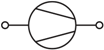
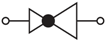


© 2017 by the authors; licensee MDPI, Basel, Switzerland. This article is an open access article distributed under the terms and conditions of the Creative Commons Attribution (CC-BY) license (http://creativecommons.org/licenses/by/4.0/).