A Cubature-Principle-Assisted IMM-Adaptive UKF Algorithm for Maneuvering Target Tracking Caused by Sensor Faults


1
Aeronautics and Astronautics Engineering College, Air Force Engineering University, Xi’an 710038, China
2
Astronautics College, Northwestern Polytechnic University, Xi’an 710072, China
*
Authors to whom correspondence should be addressed.
Appl. Sci. 2017, 7(10), 1003; https://doi.org/10.3390/app7101003
Submission received: 20 July 2017
/
Revised: 2 September 2017
/
Accepted: 26 September 2017
/
Published: 28 September 2017
Abstract
:Featured Application
The work is very effective and applicable in the fields of the maneuvering target tracking and navigations system design.
Abstract
Aimed at solving the problem of decreased filtering precision while maneuvering target tracking caused by non-Gaussian distribution and sensor faults, we developed an efficient interacting multiple model–unscented Kalman filter (IMM-UKF) algorithm. By dividing the IMM-UKF into two links, the algorithm introduces the cubature principle to approximate the probability density of the random variable, after the interaction, by considering the external link of IMM-UKF, which constitutes the cubature-principle-assisted IMM method (CPIMM) for solving the non-Gaussian problem, and leads to an adaptive matrix to balance the contribution of the state. The algorithm provides filtering solutions by considering the internal link of IMM-UKF, which is called a new adaptive UKF algorithm (NAUKF) to address sensor faults. The proposed CPIMM-NAUKF is evaluated in a numerical simulation and two practical experiments including one navigation experiment and one maneuvering target tracking experiment. The simulation and experiment results show that the proposed CPIMM-NAUKF has greater filtering precision and faster convergence than the existing IMM-UKF. The proposed algorithm achieves a very good tracking performance, and will be effective and applicable in the field of maneuvering target tracking.
1. Introduction
With the continuous development of space technology, maneuvering ability in real time is a key factor in completing complicated space missions for maneuvering targets [1,2,3,4]. Performing accurate maneuvering target tracking and precise locating are the core issues in the field of space target surveillance [5,6,7,8].
For maneuvering target tracking, the single model filter produces large filtering errors, and it is not appropriate for this application because the filtering algorithms highly depend on the motion model of the targets. The interacting multiple model (IMM) method integrates a variety of models to describe the motion rules of the targets, which improves the filtering precision. IMM was proposed by Blom and Barshalom [9], and consists of three processes: interaction, filtering, and fusion. The interaction process is the core difference between IMM and the first generation of multiple model filters, called autonomous multiple model (AMM) filters [10], which connect all the single filters organically to allow the “soft switching” between models. Due to the ability to automatically adjust the bandwidth of the filter, IMM has been widely used in navigation, positioning, signal processing, maneuvering target tracking, and other fields [11,12].
Based on the standard IMM, increasingly improved IMM algorithms have been created to further increase the filtering accuracy, including the Variable Structure Interactive Multiple Model (VSIMM) [13], Adaptive Interactive Multiple Model (AIMM) [14], and the Adaptive Grid Fuzzy Multiple Model (AGFIMM) [15]. After analysis, the above algorithms are common for all dynamic adjustments of the multi-model set and for real-time conversions between multi-model sets, in order to adapt to the real-time signal change and to improve the filter’s precision.
However, when interacting, the weighted sum of multiple random variables will lead to multiple peaks in the probability density function of the system state, so the sum will not conform to the pure Gaussian distribution [16,17]. As a result, the filtering precision is negatively influenced for the non-Gaussian distribution. Two methods are used to address the problem. The Gaussian distribution can be used to approximate the non-Gaussian distribution [18]. For example, Lainiotis uses the mean square error (MSE) to estimate the error covariance of the interacting random variable [19], but the estimated value is too conservative. Because the MSE estimation results are used in the filter iteration, it artificially increases the system noise in the filtering process, which makes the calculation value of gain matrix too large. Therefore, the filtering precision decreases, especially with a large measured value of noise [20]. The second method is to filter the results of the interaction by using non-Gaussian filters [21]. For instance, the IMM-PF filtering method [22,23] can be used, but the particle filter (PF) causes problems, such as particle degradation and poor real-time performance, in engineering applications [24,25].
The unscented Kalman filter (UKF) is the most widely used algorithm with a single filter in the IMM [26,27,28,29,30,31,32], and has many advantages compared to the Kalman Filter (KF), Extended Kalman Filter (EKF) [33,34], and PF. However, the tracking accuracy decreases significantly when sensor faults occur, because model mismatches are produced when the sensor receives measurements with biases [35,36,37]. Generally, the sensor faults include four varieties: complete failure, fixed deviation, drift deviation, and accuracy decrease. The second and third faults are considered in this research. The current existing adaptive UKF has been proven to be effective in dealing with unknown noise, but no effective adaptive UKF algorithms exist for sensor faults and model mismatches [38,39].
Recently, Arasaratnam et al. [40] proposed the cubature Kalman filter (CKF), based on the cubature principle, and provided rigorous mathematical proof. The cubature principle is the basis of CKF, and it computes the first and second order moments of the finite cubature points through nonlinear propagation, and then estimates the posterior probability density of the nonlinear system. As a typical deterministic sampling filtering algorithm, CKF has fewer sampling points and better numerical stability [41]. As the mixed probability of IMM interaction varies with time, the interaction process is described by nonlinear equations, and the cubature principle in CKF is used to estimate the probability density function of a random variable after the interaction. To address the single model filtering precision problem, a new adaptive matrix gene is used in UKF together with the IMM method, to balance the contribution of the state and filtering results in the presence of sensor faults.
This paper develops a new efficient IMM-UKF algorithm for maneuvering target tracking, which addresses the non-Gaussian distribution problem and sensor faults. The IMM-UKF filtering problem is described for maneuvering target tracking with the occurrence of sensor faults. For IMM-UKF external links, the cubature principle (CP) is introduced to IMM to approximate the probability density of the random variable in the interaction, and the precision of the approximation is analyzed, which contributes to CP-assisted IMM (CPIMM). For IMM-UKF internal links, an adaptive matrix gene is integrated into traditional UKF to balance the contribution of the system state and provides filtering solutions, which is called a new adaptive UKF (NAUKF). Simulation and experiment results showed that the proposed cubature principle assisted IMM–adaptive UKF algorithm (CPIMM-NAUKF) has high filtering precision and fast convergence, and achieves better tracking performance than the existing IMM-UKF.
2. Description of the IMM-UKF Filtering Problem
2.1. Maneuvering Target Tracking Dynamic System
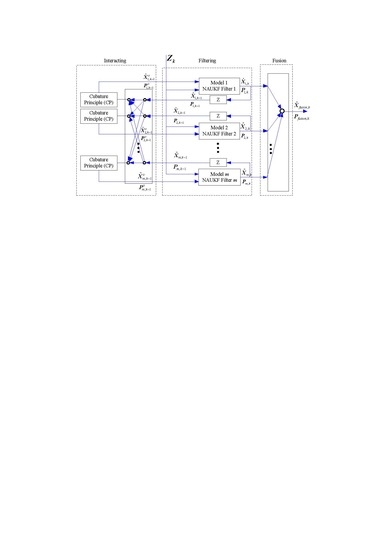
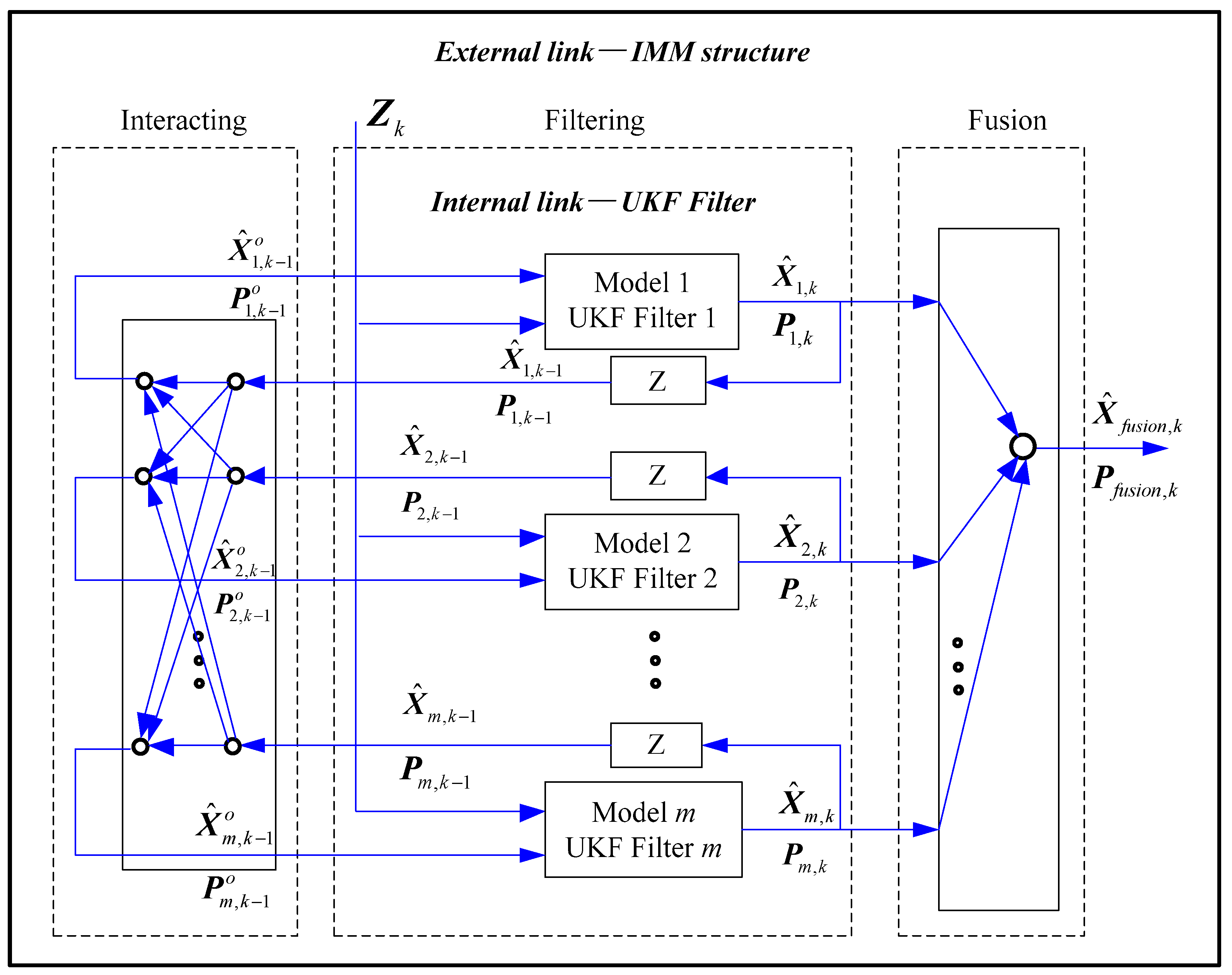
The general IMM-UKF structure diagram, including models, is shown in Figure 1, where represents the unit delay link. The IMM-UKF can be divided to two parts: the external link-IMM structure and the internal link-UKF filter.
In Figure 1, and are the state estimation and covariance matrix, respectively, of the single UKF filter at time step ; and are the corresponding vector at time step ; and are the interaction result of and , and they are the inputs of UKF filter ; and are the final state estimation and covariance of the IMM-UKF filter, respectively; and denotes the measurement vector for the single UKF filter.
For single model , the state and measurement equations of the maneuvering target are [1,4]
where the subscript is omitted for the sake of brevity.
Similarly, the state and measurement equations of the maneuvering target in the presence of sensor faults are [35,37]
where and represent the state transfer function and interference transfer matrix, respectively; and denote the system and measurement noise, respectively, and they are both white Gaussian noises and mutually uncorrelated; is a nonlinear coordinate transformation function; and denotes the model mismatches caused by sensor faults.
2.2. Standard IMM
Step 1: Model probability updating. The mixing probability is defined and calculated as
where is the transition probability; is the correct probability of model at time step ; and is the prediction probability of model from time step to time step [11] which provides
Therefore, we can obtain the updated model probability:
where ; ; represents the innovation residual vector of UKF filter ; and represents the covariance matrix of .
Step 2: Input interaction.
where .
Step 3: Resultant mean and covariance matrix computation.
2.3. Non-Gaussian Distribution and Sensor Fault Problems for IMM-UKF
2.3.1. Non-Gaussian Distribution
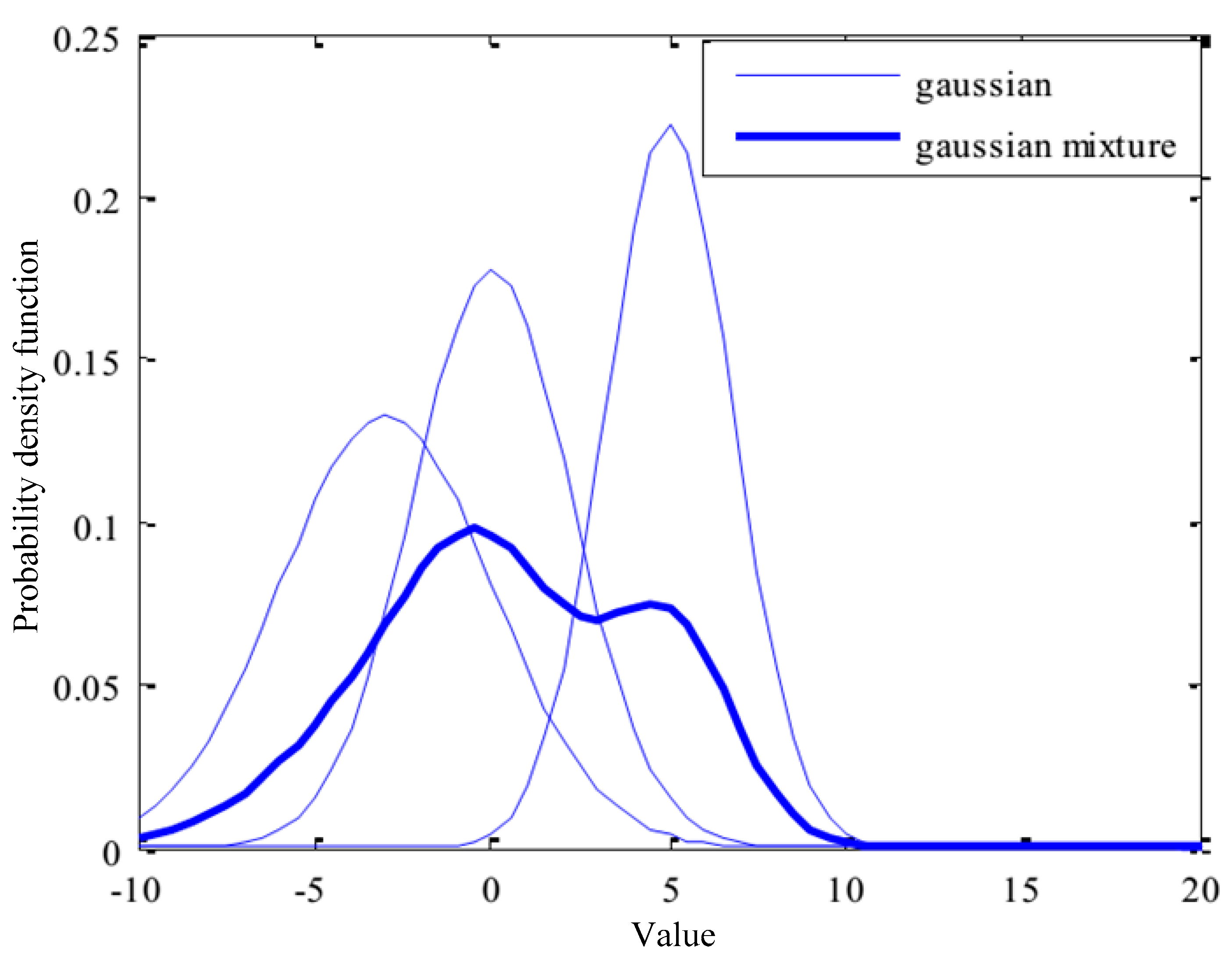
For the external IMM-UKF links, is a weighted sum of Gaussian random variables and no longer obeys the pure Gaussian distribution because many peaks will exist in the probability density, which is similar to the probability density of the mixed Gaussian distribution [19]. The case when is scalar and is constant is explained in this section. It is assumed that is the weighted sum of three Gaussian random variables with normal distribution, and is the square root of , where , , . The probability density of the mixed Gaussian distribution is shown in Figure 2.
In Figure 2, the thick line represents and has multiple peaks; the mixture no longer follows Gaussian distribution.
After the interaction, Lainiotis completes the approximation of the probability density through the Gaussian distribution [19]:
where is the square root of .
On the basis of the above distribution, MSE estimates the covariance matrix of the interacting random variables, where the mean and covariance matrix are computed by [16]
From Equations (11) and (12), we know is larger than the actual covariance of (). An example of the above one-dimensional case is available, and the Monte Carlo method (MC) is used with 10,000 random sampling points to compute the mean and covariance transferred. The results are shown in Table 1.
From Table 1, is verified. Because will participate in the filtering iteration, it is equivalent to an increase of the system noise in the process of filtering. Then, the gain matrix will be larger, and the filtering effect declines, especially when the actual system noise is small and the measurement noise is large.
Therefore, for the external IMM-UKF link, the filtering problem to be solved is how to make a precise estimate of the mean and covariance matrix of the random variables after the interaction for IMM.
2.3.2. Sensor Faults
When sensor faults exist, the third-order accuracy condition is no longer met for the standard UKF [42]. Therefore, for the internal IMM-UKF link, the filtering problem to be solved is how to design an effective adaptive UKF algorithm for systems given by Equation (2), when the sensor fault exists.
3. Cubature-Principle-Assisted IMM-Adaptive UKF Algorithm (CPIMM-NAUKF)
By considering the internal and external link of IMM-UKF respectively, the cubature principle is introduced to the standard IMM, and an adaptive gene matrix is brought into the standard UKF.
For IMM, the most important factor on influencing the filtering precision is the non-Gaussian probability density function after the mixing interaction. It is the key to estimating the first moment and second moment of the random variables with high accuracy.
For adaptive UKF, one effective method is to balance contribution to UKF filtering solutions of the state information, measurement information, and innovation information.
3.1. CPIMM
3.1.1. Cubature Principle
Assuming that , where the dimension of is , then the first moment and second moment of any function can be solved by the following integral form:
Equation (13) is a multidimensional integral problem, and it is difficult to solve through analytic methods. The cubature principle states that a cubature point with a weighted value can be chosen to approximate the integral of the multidimensional function, and the method of choosing the cubature point is:
where is the rth column of the unit matrix .
3.1.2. Estimating the Interaction by Using CP
Since the mixing probability varies with time, the interactive process is abstracted as a nonlinear function, and the cubature principle is used to approximate the probability distribution of the interacting random variables.
Firstly, the nonlinear function is used to describe the interaction process. The augmented system is constructed, where is a random variable with the dimension, and represents the state vector of the model ; ; . Assuming that is independent, and we have , the square root of the covariance matrix of is , and we have .
The next step is choosing cubature points for nonlinear propagation. The cubature points are selected by Equation (13), and is rewritten as , where is the upper triangular matrix with all the diagonal elements being ; is the value of the element on the diagonal of , and the cubature points can be written as
where is the rth column of .
The cubature points are calculated after the interaction by
Finally, according to the cubature principle, the mean and covariance matrix of are obtained as
where ; .
For the external IMM, shown by Equation (6) can be recalculated by Equation (18), and shown by Equation (7) can be recalculated by Equation (19); then, the newly obtained and are used in the iteration of the IMM filter, which leads to CP-IMM.
3.1.3. Accuracy Analysis of the CPIMM
In the literature [22], the approximate precision of the mean of the Gaussian random variable after nonlinear propagation, by using the cubature principle, has been analyzed. In this section, the accuracy of the covariance matrix of the cubature principle will be analyzed.
Assume that is the nonlinear mapping from to ; ; . If the Taylor series expansion of is carried out at with two derivatives, we have
where is the Jacobian matrix with a dimension; represents matrixes with dimensions, which are called Hessian matrixes; is the Hessian matrix. Thus, we have
Calculating the first and second moments of Equation (20), we obtain
where represents the trace of a matrix.
Equation (18) can be rewritten as
Substituting Equation (23) to (19), and assuming , we have
When is correct by considering the selection process of cubature points shown in Equation (17), we have
Substituting Equation (25) into Equations (23) and (24), respectively, we obtain
Equations (22) and (26) show that the mean and covariance estimates can achieve second-order accuracy of a Taylor series expansion using the cubature point to create a random variable through the nonlinear function. The one-dimensional case in Section 2.3 is used to illustrate that the mean value obtained by the cubature principle is 0.6, and the covariance is 1.3826, which is much closer to the results obtained by Monte Carlo method than the MSE method.
3.2. New Adaptive Unscented Kalman Filter (NAUKF)
Motivated by the proposed UKF algorithm, we propose a new adaptive UKF (NAUKF) consisting of an adaptive matrix gene. , and represent the corresponding covariance computed by the standard UKF, and they are changed into , and in the NAUKF.
Theorem 1.
On the basis of standard UKF, set up a new adaptive matrix gene as
Let
where is calculated from the Sigma points in the standard UKF; is the innovation; denotes the weighted coefficient [3]; ; and is the covariance of ; Then the NAUKF can address the filtering problem in the presence of sensor faults shown by Equation (2).
Proof:
Because model mismatches exist in the system shown by Equation (2), based on Theorem 1, the result is
where .
After setting up shown by Equation (27), we have
From Equations (29) to (31), we know that the third-order precision conditions can be satisfied, which means that the NAUKF can be used for the system that has sensor faults. This completes the proof.
To avoid the divergence problem of NAUKF, a covariance matching criterion is used:
where () is a preset adjustable coefficient.
If Equation (32) is satisfied, the NAUKF has been convergent; should be updated with an adaptive weighted coefficient by increasing the contribution of on the filtering solutions.
where is set by
3.3. Implementation Steps of the CPIMM-NAUKF Algorithm
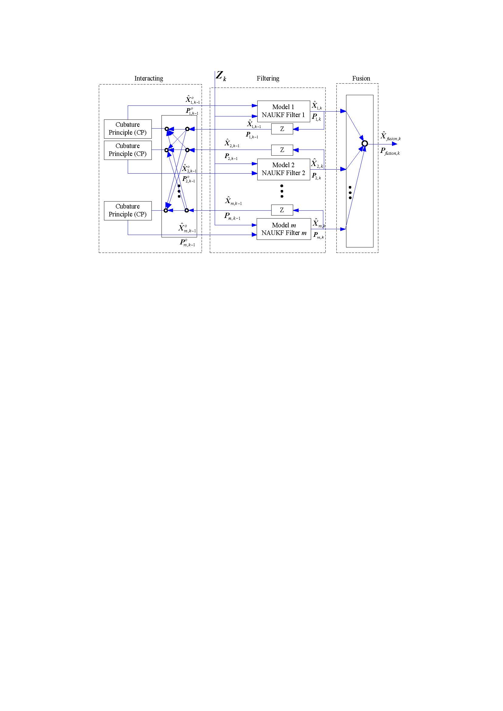
Based on Section 3.1 and Section 3.2, the CPIMM-NAUKF structure is shown in Figure 3. The implementation steps of the CPIMM-NAUKF are as follows.
Step 1: NAUKF filtering process.
First, calculate the covariance by setting and of the standard UKF, and compute . Next, select the new adaptive gene selection by setting up through Equation (27), and recalculate with Equation (28)
To determine the convergence strategy, judge the divergence according to Equation (32). If it is satisfied, go directly to the next step; otherwise, update by using Equations (33)–(35).
Next, to obtain the NUKF filtering results, use the following:
From Equations (38) and (39), obtain the , , …, and for UKF filters to of IMM-UKF.
Step 2: The CPIMM filtering process.
First, compute the mixing probability. Calculate the mixing probability according to Equation (3). Next, determine the Interaction by using CP. After , , …, and are obtained based on Step 1, calculate and , respectively, with Equations (18) and (19). Then update the model probability by calculating the mixing probability according to Equation (5). To complete the fusion, calculate resultant mean and covariance matrix with Equations (8) and (9).
4. Experimental Results and Discussion
To verify the effectiveness of the maneuvering target tracking of the proposed CPIMM-NAUKF, numerical simulations and practical experiments are both conducted. For the numerical simulation, two sets of experiments were simulated: (1) the standard IMM [9] and CPIMM algorithms; (2) the IMM-UKF [43], IMM-NAUKF connecting the standard IMM with NAUKF, CPIMM-UKF connecting the CPIMM with standard UKF, and CPIMM-NAUKF algorithms. The experimental environment was set as Intel i7 computer with 4-core, 64-bit, 2.4 GHz, 8 GB RAM, and MATLAB R2013a software. For the practical experiments, an integrated navigation system and a synthetic aperture radar (SAR) tracking system using the CPIMM-NAUKF algorithm are, respectively, shown to test the proposed method with real data.
4.1. Numerical Simulations and Analysis
To design the simulation scenarios, suppose that represents the state of the maneuvering target, including the position and velocity. The sensor is the radar, and its position is fixed at the coordinate origin. Thus, the measurement equation is
where and are the distance and angle measurement components of the radar, respectively.
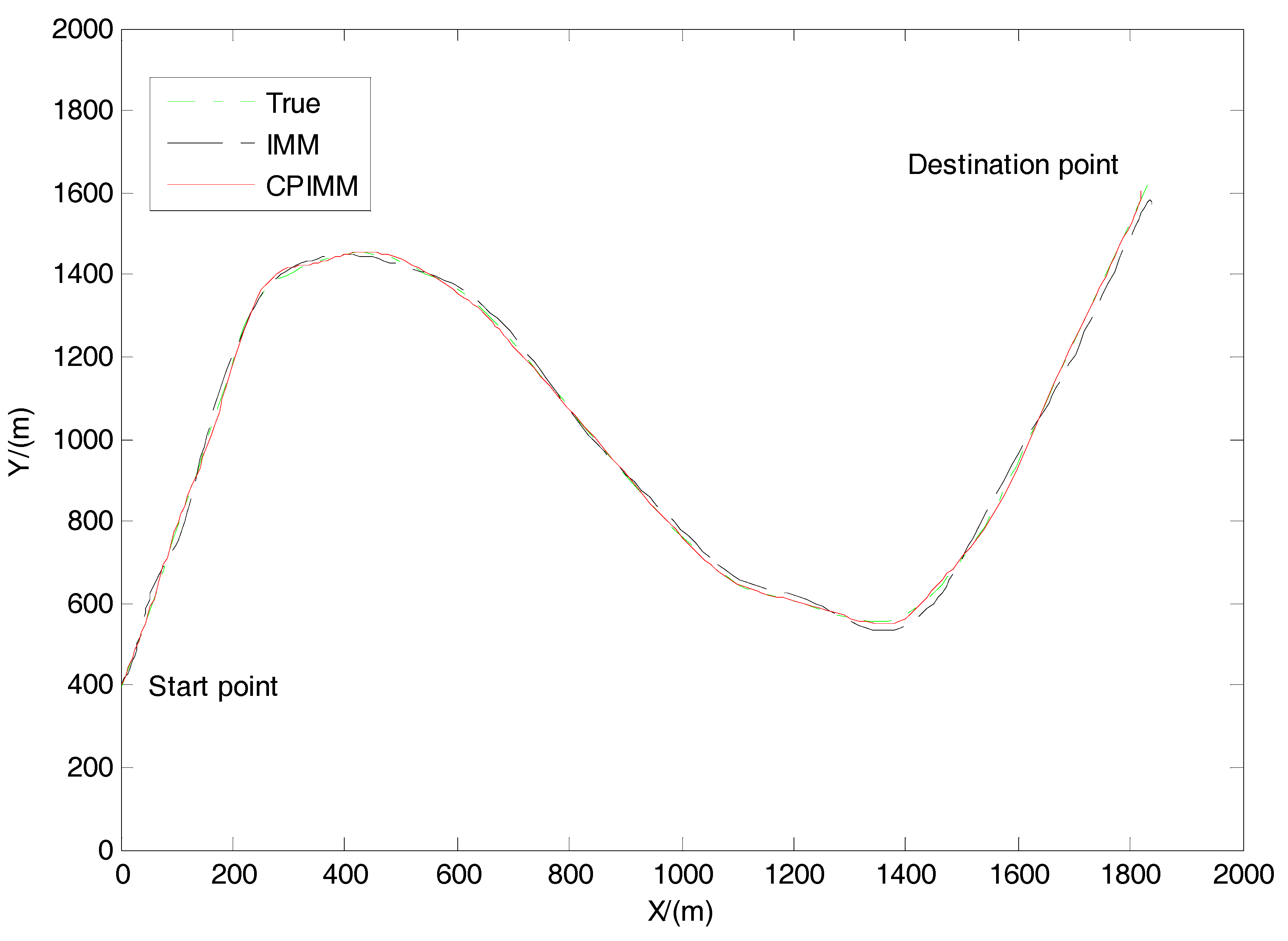
The high-speed maneuvering target moves in a two-dimensional scenario with 100 s; the initial position is [0 m, 400 m], and the initial velocity is [10 m/s, 40 m/s]; the target moves at a constant velocity in a straight line from 0 s–20 s, with a constant right turn rate being −0.1 rad/s from 20 s–40 s, constant velocity in a straight line at 40 s–60 s, constant left turn with the turn rate being 0.1 rad/s at 60 s–80 s, and a constant velocity in a straight line at 80 s–100 s. In a Cartesian coordinate system, the true trajectory of the maneuvering target is depicted in Figure 4.
Both the IMM and CPIMM include three models: one Constant Velocity (CV) model [44] and two Coordinated Turn (CT) models [44].
For the CV model, the state transition matrix is
where T is the sampling period, and T = 1 s.
The process noise is calculated with
where denotes the covariance of the process noise, and .
For the CT model, the state transition matrix is
where is the turn rate.
The process noise meets with
where denotes the covariance of the process noise, and .
The two models use the following transition and mode probabilities.
The transition probability matrix is
The initial mode probability matrix is
The measurement covariance is .
Case 1 is where the sensor has no faults and is in a normal work situation. Case 2 is when the sensor has faults, and , where and represents the distance deviation within [−5 m, 5 m] and the angle drift rate within , respectively.
Every simulation experiment is tested 100 times using Monte Carlo, and algorithms of two sets of comparison simulations are evaluated by root mean square error (RMSE), which is computed through
where and are the estimated and true state in the simulation, respectively; is the number of simulations; .
4.1.1. CPIMM Simulation
To validate the effectiveness of CPIMM, the first set of comparisons, including the standard IMM and CPIMM, was simulated. We assumed there were no sensor faults, similar to the Simulation Case 1 in the scenario design section.
Figure 5 gives the true and estimated trajectories of the maneuvering target. As seen in Figure 5, both CPIMM and IMM can track the trajectory of the target.
The comparisons of the RMSE position and velocity curves of the two filtering algorithms are shown in Figure 6 and Figure 7, and the corresponding statistical data of RMSE are listed in Table 2. The filtering precision of the IMM is lower than the CPIMM, although the IMM is not divergent. The CPIMM greatly increases the filtering precision compared with IMM. In addition, this means that the tracking performance of CPIMM is higher than that of the IMM, because the cubature principle is used to increase the estimation values in the interaction process of the IMM.
4.1.2. CPIMM-NAUKF Simulation
To validate the effectiveness of CPIMM-NAUKF, the second set of comparisons, including the IMM-UKF, IMM-NAUKF, CPIMM-UKF, and CPIMM-NAUKF were simulated, assuming there are sensor faults, similar to Simulation Case 2 in the scenario design section.
Figure 8 gives the true and estimated trajectories of the maneuvering target. Both CPIMM and IMM can track the trajectory of the target, but the estimated trajectory of CPIMM-NAUKF was closest to the true trajectory.
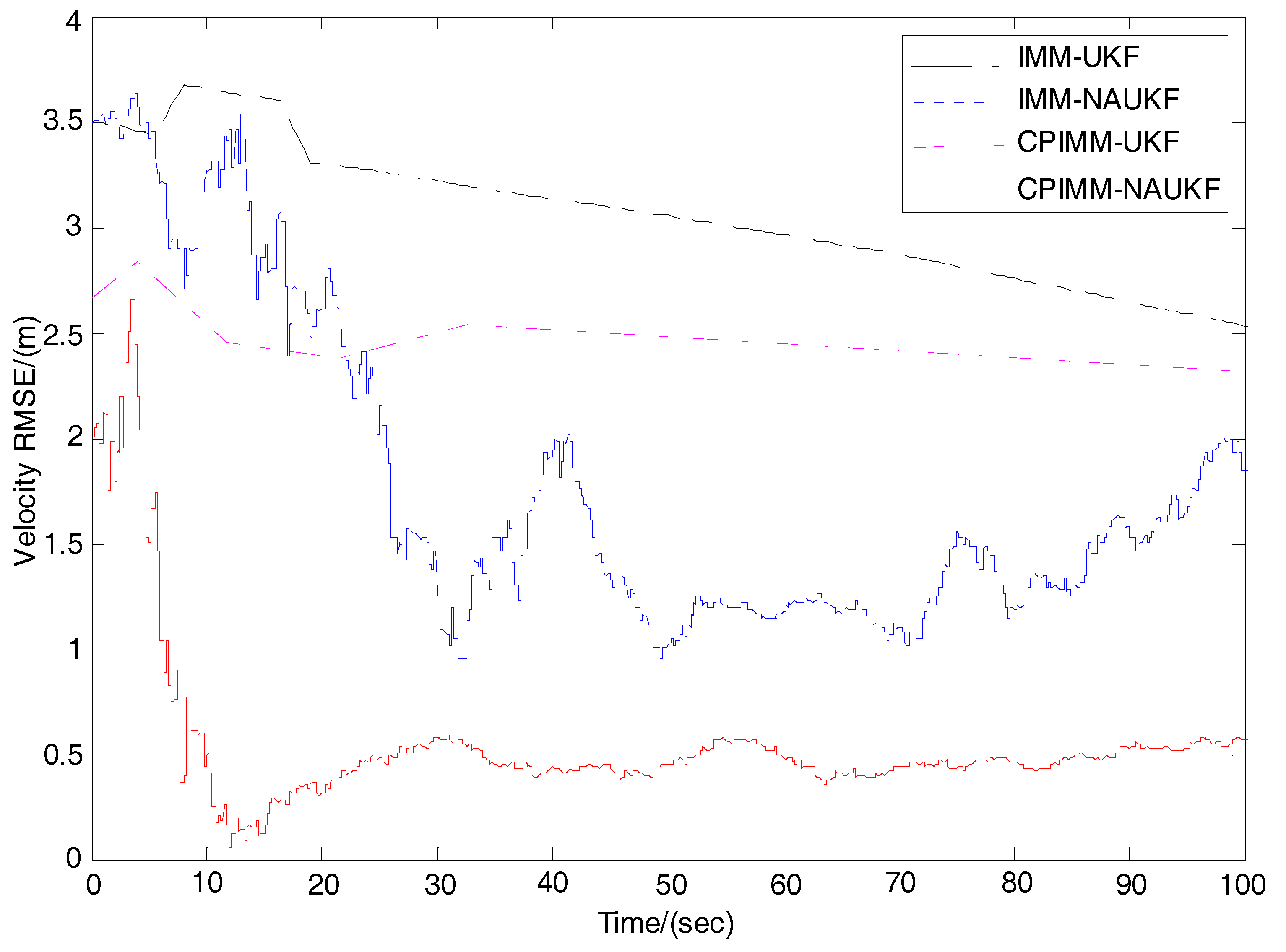
The comparisons of the RMSE position and velocity curves of four filtering algorithms are shown in Figure 9 and Figure 10, and the corresponding statistical data of RMSE are listed in Table 3. The sensor faults negatively influenced the filtering precision of the UKF and the filtering error of the standard IMM-UKF was the largest. The IMM-NAUKF has better filtering accuracy than the IMM-UKF, because the internal link NAUKF effectively handled the sensor fault problem, but the filtering convergence performance was poor. The CPIMM-UKF also has better filtering accuracy than the IMM-UKF because the internal link CPIMM has a better effect for maneuvering target tracking than IMM, but the filtering accuracy relationship between IMM-NAUKF and CPIMM-UKF does not exist. Ultimately, CPIMM-NAUKF has the best filtering accuracy, since it significantly improves the IMM-UKF through the external and internal links, which makes it extremely effective for maneuvering target tracking when sensor faults occur.
In summary, as a combination of CPIMM and NAUKF, the CPIMM-NAUKF, compared with the existing IMM-UKF, makes a greater contribution to filtering performance in terms of accuracy and convergence speed. This is because it includes two important links, the external CPIMM and the internal NAUKF, which work simultaneously and effectively.
4.2. Practical Experiments and Analysis
Furthermore, to demonstrate the effectiveness of the proposed CPIMM-NAUKF method for real applications, two practical experiments were conducted. An unmanned aerial vehicle (UAV) was loaded with an Inertial Navigation System (INS)/Global Positioning System (GPS) integrated navigation system for its navigation and positioning, and equipped with an SAR tracking system to track the maneuvering targets.
4.2.1. INS/GPS Integrated Navigation System
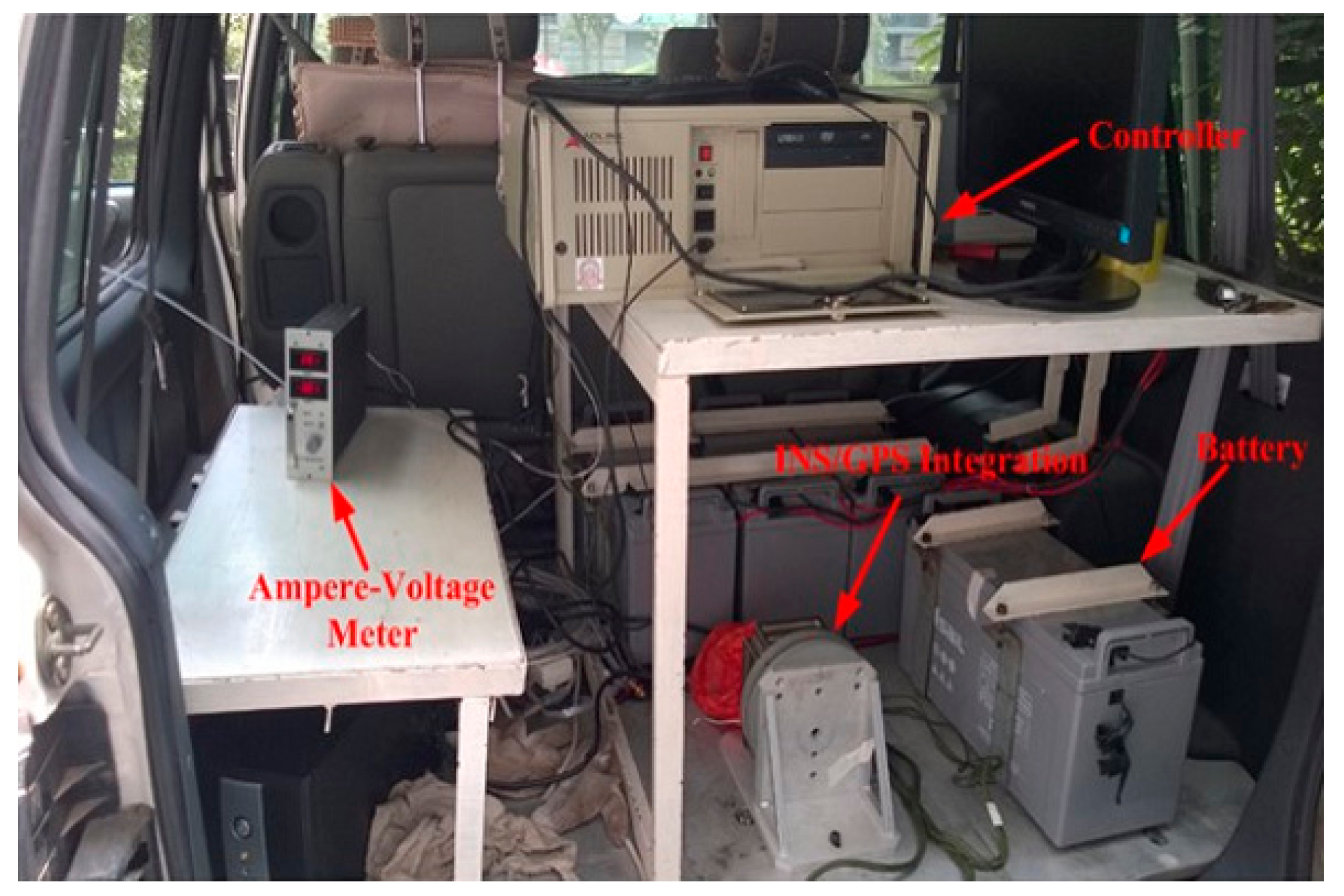
As shown in Figure 11 and Figure 12, the vehicle loaded integrated navigation system included a NV-IMU300 type INS, a JAVAD Lexon-GGD112T type GPS receiver, and a NovAtel DL-V3 GPS receiver on the vehicle, and another NovAtel DL-V3 GPS receiver was located at the Earth Reference Station. The working frequency of the GPS was 20 Hz. The maximum distance between the vehicle and the Earth Reference Station had to be less than 60 km, which ensured that the positioning precision of the vehicle was better than 0.1 m.
Let the geographic coordinate system be the navigation coordinate system with three directions of East, North, Up. Define the system states as
where represent the heading angle, the pitch angle, and the roll angle of the vehicle, respectively; are components of the velocity along the East, North, and Up directions, respectively; are components of the position along the East, North, and Up directions, respectively; represent the drift of the gyro; represent the bias of the accelerator.
The state space model is
the concrete equations of which can be found in [45].
Select the velocity and position outputs of the GPS as the measurement variables:
where are components of the velocity measured via GPS along the East, North, and Up directions, respectively; are components of the position measured via GPS along East, North, and Up directions, respectively. The velocity and position information measured via GPS can be used as a reference to confirm the position error of the INS/GPS.
The measurement equation is
where .
In the experiment process, the initial position was as follows: East longitude 108.891227°, North latitude 34.286866°, and an altitude of 437.92 m. Components of the velocity along the East, North, and Up directions were, respectively, −8 m/s, −35 m/s, and 0 m/s; the drift of the gyro was 0.12°/h, and the white noise was 0.02°/h; the bias of the accelerator was 10−3 g, and the white noise was 10−4 g; the positioning and position precision of the GPS were 5 m and 0.05 m/s; the other initial parameters were the same as the those described in the simulation section. The experiment test time was designed as 500 s with the sample period being 1 s, and the end point of the vehicle was East longitude 108.995683°, North latitude 34.285292°, and an altitude of 438.01 m. The practical road condition was the urban highway, and the real route of the vehicle is shown in Figure 13.
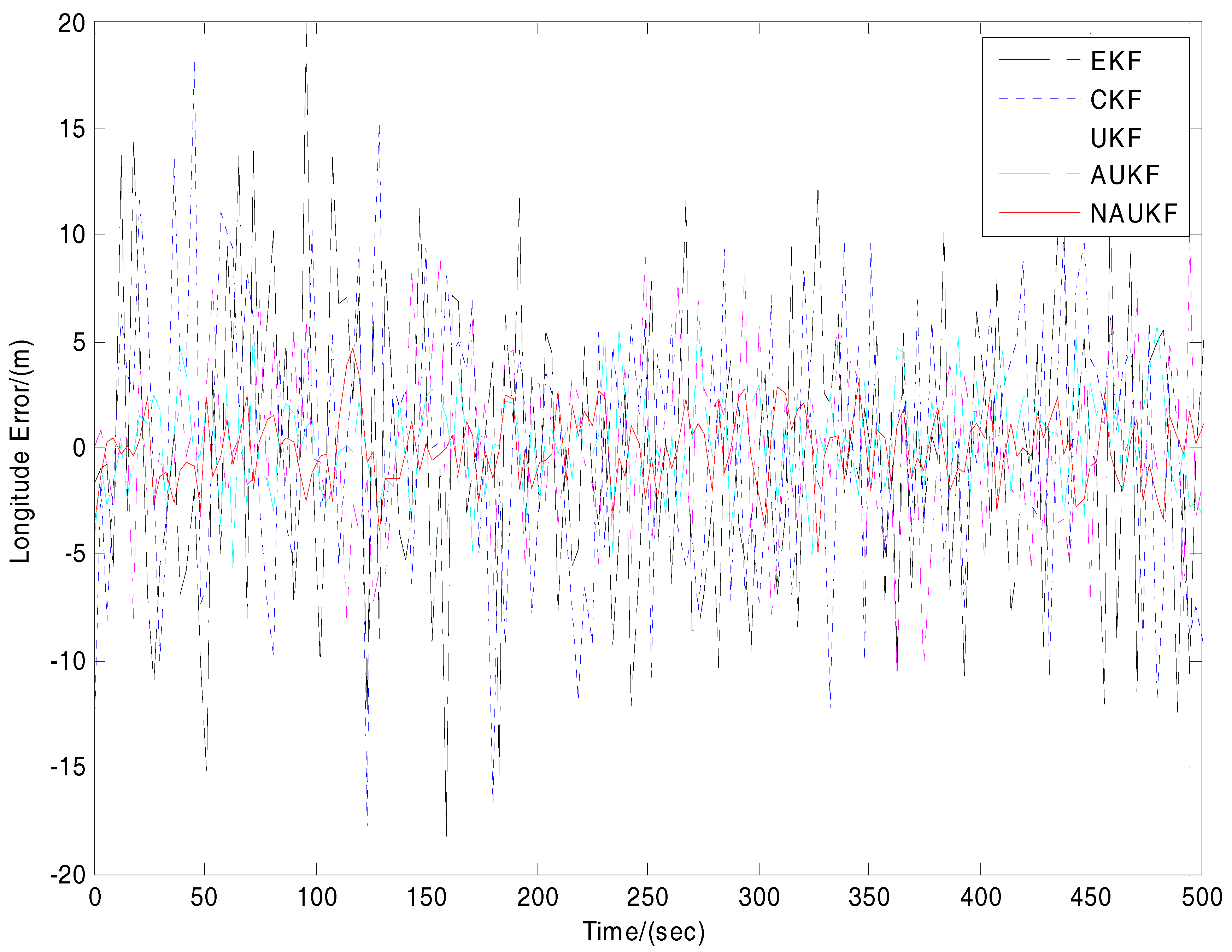
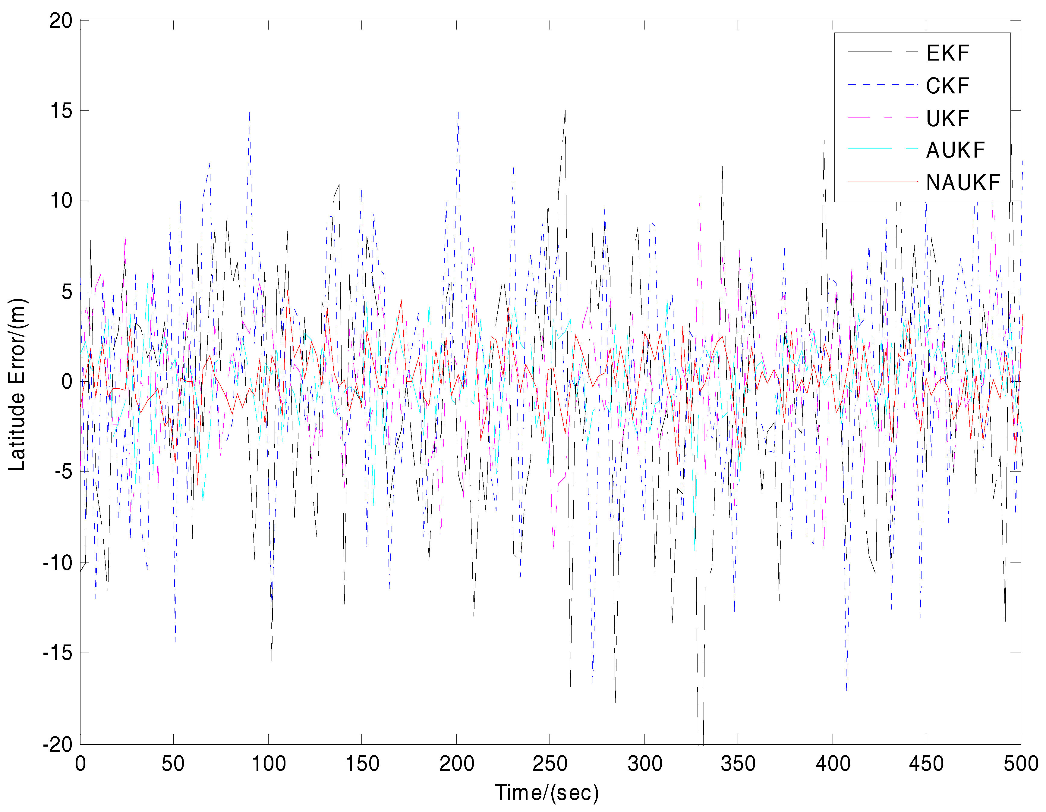
Five filtering methods including standard EKF [33], CKF [40], standard UKF [27], existing adaptive UKF (AUKF) [38], and NAUKF were used in the experiment, and these algorithms were evaluated by the estimation error rather than RMSE, which is computed through
The comparisons of the longitude and latitude error curves of five filtering algorithms are shown in Figure 14 and Figure 15, and the corresponding statistical data of the mean absolute error are listed in Table 4. We can see that the EKF and CKF have almost the same filtering accuracy, although both EKF and CKF can deal with the nonlinear filtering problems—they only have first order accuracy. The filtering errors are, respectively, [−18.1025, 19.9471] m and [−17.5118, 18.4296] m of the longitude error ranging, and [−20.1143, 16.2477] m and [−17.4154, 14.9953] m of the latitude error ranging. The standard UKF has better filtering precision than does EKF and CKF, because UKF can reach third order accuracy, but it still has substantial oscillation and error due to the longitude error ranging [−11.0549, 10.2178] m and latitude error ranging [−9.1766, 9.9737] m. The AUKF has the adaptive ability of the imprecise noise in the urban complex environment, so it has better filtering accuracy than the UKF with the longitude error ranging [−5.8142, 6.0273] m and latitude error ranging [−8.1184, 6.4153] m. Ultimately, NAUKF has the best filtering accuracy, with the longitude error ranging [−4.1109, 4.3804] m and latitude error ranging [−6.1096, 4.7138] m, since it can not only adapt to the noise but also the sensor faults and model mismatches.
In summary, UKF has better filtering precision than KF, EKF, and CKF, because UKF can reach third order accuracy. The proposed NAUKF has the best filtering performance in terms of precision and dynamic response for its adaptive ability to both imprecise noise and sensor faults, and it can increase the precision and adaptability of the navigation system effectively.
4.2.2. SAR Tracking System
As shown in Figure 16 and Figure 17, the UAV is equipped with one D3160 type SAR. The UAV is a six-rotor UAV with mass being 20 kg and velocity range being 0 m/s–20 m/s. The D3160 type SAR is a kind of micro-SAR system and the parameters are as follows: mass: 4 kg, operating frequency band: X or Ku, detection range: 10 km, resolution: 0.3 m.
The SAR can detect the pitch angle , azimuth and distance of the target vehicle relative to the UAV, and the measurement equation is
where is the position of UAV; is the position of the target vehicle.
In the experiment process, both the pitch angle and azimuth measurement had the drift rate, and the distance measurement had the deviation for the SAR, but the precise statistics about the sensor faults and noises are still unknown. In Figure 18, the target vehicle is driving on the expressway, and the initial position of the UAV and the target vehicle is, respectively, East longitude 108.933195°, North latitude 34.188183°, and an altitude of 1.50 km and East longitude 108.938962°, North latitude 34.187501°, and an altitude of 436.05 m. The experiment test time is designed as 1000 s with the sample period being 1 s, and the end point of the UAV and the target vehicle is, respectively, East longitude 109.130943°, North latitude 34.245275°, and an altitude of 1.50 km and East longitude 108.145231°, North latitude 34.239740°, an altitude of 436.76 m.
When the IMM and CPIMM methods are used, the target model description is the same as the numerical simulation. Four filtering methods including IMM-UKF, IMM-NAUKF, CPIMM-UKF, and CPIMM-NAUKF were used in the experiment, and these algorithms were evaluated by the estimation error shown by Equation (50).
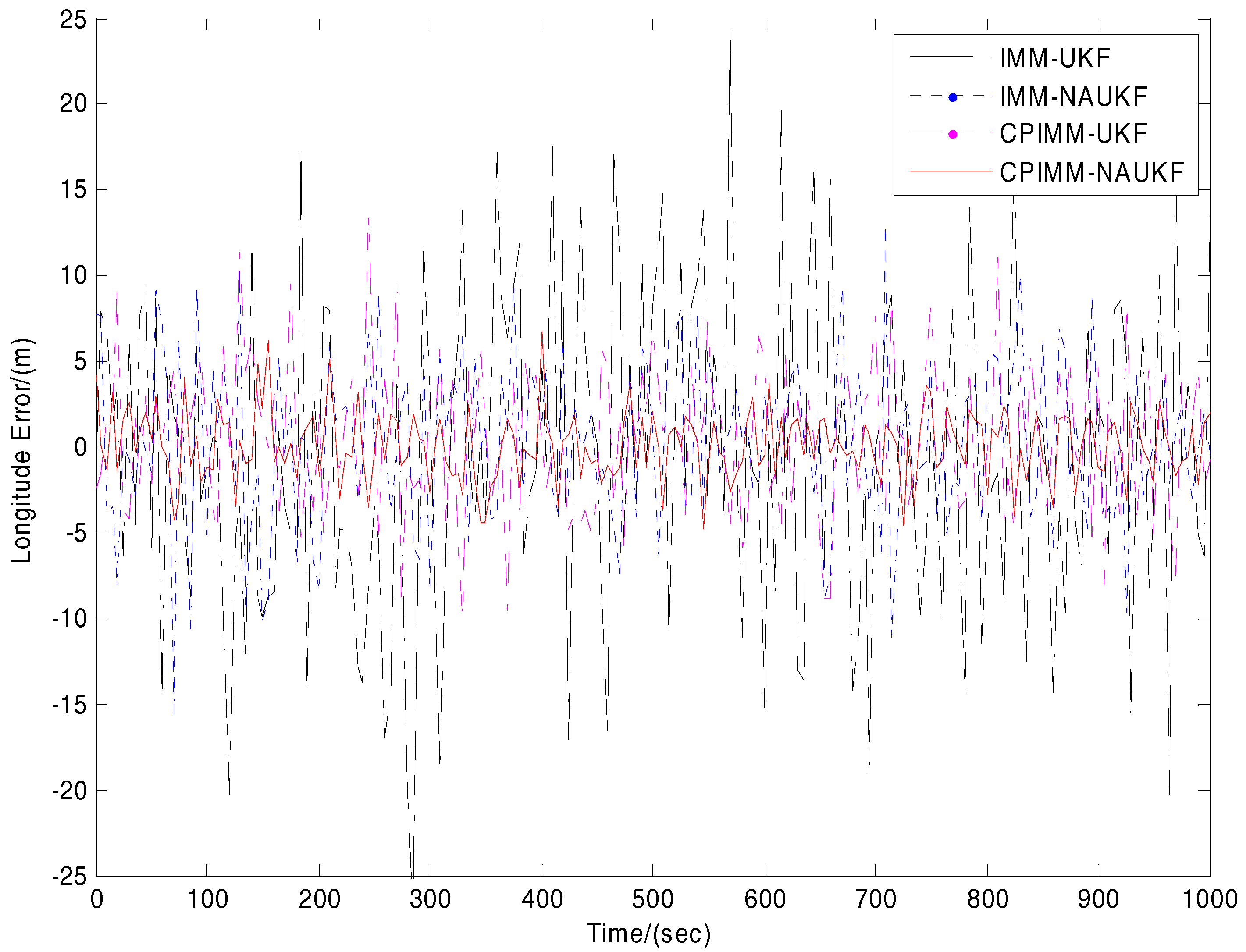
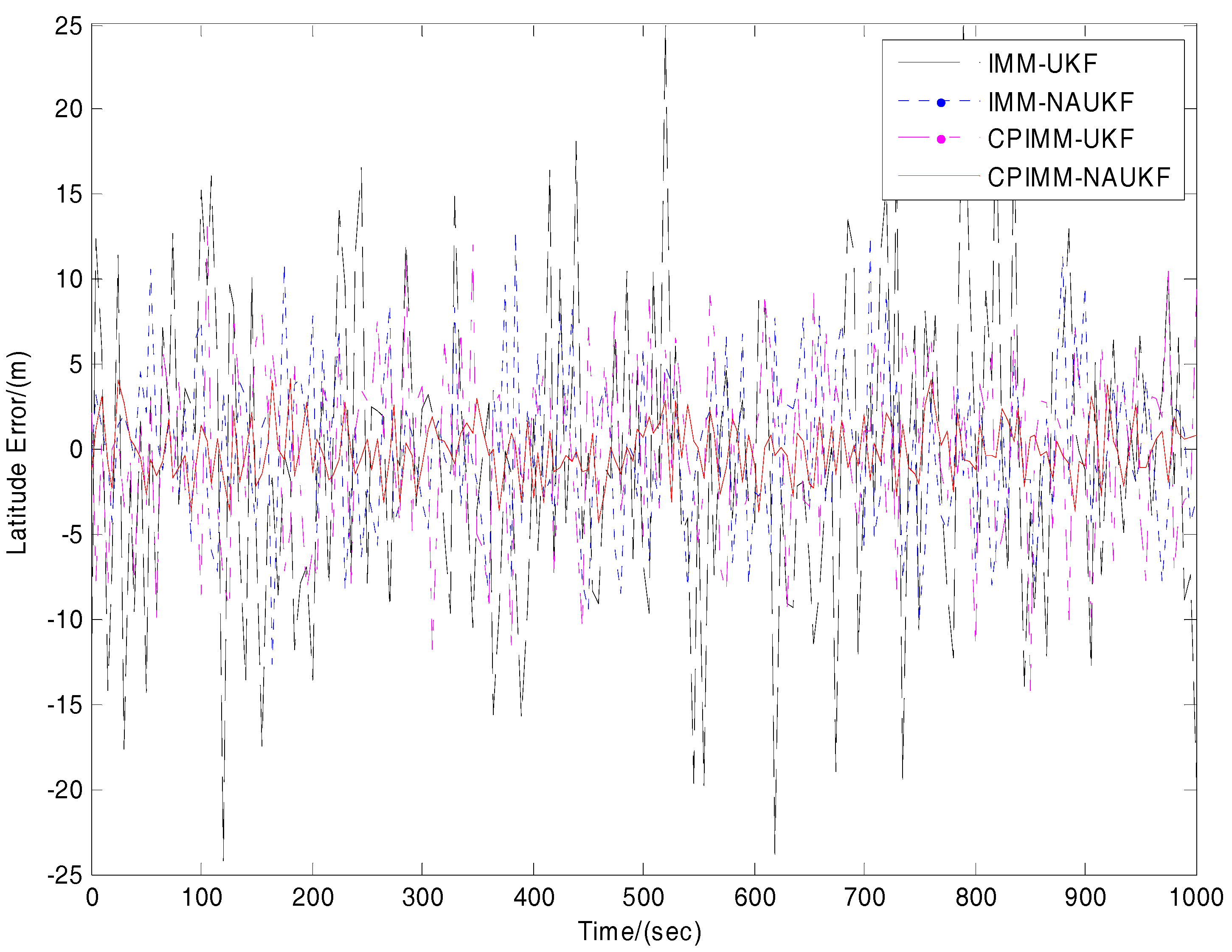
The comparisons of the longitude and latitude error curves of five filtering algorithms are shown in Figure 19 and Figure 20, and the corresponding statistical data of the mean absolute error are listed in Table 5. We can see that the standard IMM-UKF has the biggest filtering error with the longitude error ranging [−25.0223, 24.8762] m and latitude error ranging [−23.9917, 24.9834] m. The IMM-NAUKF has better filtering precision than IMM-UKF because of the adaptive ability to the sensor faults with the longitude error ranging [−16.1849, 14.0871] m and latitude error ranging [−13.8628, 14.0563] m. The CPIMM-UKF has better filtering precision than IMM-UKF because of the adaptive ability to the non-Gaussian distribution with the longitude error ranging [−10.0547, 14.2482] m and latitude error ranging [−14.7196, 12.2544] m. The CPIMM-NAUKF has the best filtering accuracy, since it can not only adapt to the non-Gaussian but also the sensor faults and model mismatches with the longitude error ranging [−5.0018, 6.8623] m and latitude error ranging [−4.8007, 4.9106] m.
In summary, the practical experiments results demonstrate that the proposed CPIMM-NAUKF is obviously superior to the existing IMM and UKF algorithms in terms of filtering precision and dynamic response for its adaptive ability to both non-Gaussian and sensor faults, and it can significantly improve the precision and robustness of the maneuvering target tracking system.
5. Conclusions
Maneuvering target tracking is a key technology and research hotspot in the field of navigation, guidance, and control. This paper proposes an efficient IMM-UKF, called CPIMM-NAUKF, for maneuvering target tracking. In the external link of CPIMM-NAUKF, the mean and covariance matrix can be calculated with high estimation precision by introducing the cubature principle, which solves the non-Gaussian problem. In the internal CPIMM-NAUKF link, the contribution of system states and innovations on the filtering solution can be balanced by introducing an adaptive matrix gene, which addresses the sensor faults. The proposed algorithm was evaluated in a classical maneuvering target tracking numerical simulation and two practical experiments including one navigation experiment with INS/GPS and one target tracking experiment with SAR. Simulation results validate that the proposed CPIMM-NAUKF improves the filtering performance in terms of higher accuracy and faster convergence, and tracks more effectively. In our future research, we will focus on the difference between UKF and other nonlinear filtering algorithms of various noise strengths.
Acknowledgments
This work was supported by the National Natural Science Foundation of China (No. 61601505), National Aviation Science Foundation of China (No. 20155196022) and the Shaanxi Natural Science Foundation of China (No. 2016JQ6050).
Author Contributions
Huan Zhou and Hui Zhao provided insights into formulating the ideas and designed the algorithm. Hanqiao Huang performed the simulations. Xin Zhao reviewed the manuscript and gave suggestions in the proposed method.
Conflicts of Interest
The authors declare no conflict of interest.
References
- Matveev, A.S.; Semakova, A.A.; Savkin, A.V. Tight circumnavigation of multiple moving targets based on a new method of tracking environmental boundaries. Automatica 2017, 79, 52–60. [Google Scholar] [CrossRef]
- Fan, Y.; Lu, F.; Zhu, W.; Bai, G.; Yan, L. A Hybrid Model Algorithm for Hypersonic Glide Vehicle Maneuver Tracking Based on the Aerodynamic Model. Appl. Sci. 2017, 7, 159. [Google Scholar] [CrossRef]
- Cao, Y.; Wang, G.; Yan, D.; Zhao, Z. Two Algorithms for the Detection and Tracking of Moving Vehicle Targets in Aerial Infrared Image Sequences. Remote Sens. 2016, 8, 28. [Google Scholar] [CrossRef]
- Leven, W.F.; Lanterman, A.D. Unscented Kalman Filters for Multiple Target Tracking With Symmetric Measurement Equations. IEEE Trans. Autom. Control 2009, 54, 370–375. [Google Scholar] [CrossRef]
- Song, Y.; Zhang, B.; Zhao, K. Indirect neuroadaptive control of unknown MIMO systems tracking uncertain target under sensor failures. Automatica 2017, 77, 103–111. [Google Scholar] [CrossRef]
- Wu, J.; Li, K.; Zhang, Q.; An, W.; Jiang, Y.; Ping, X.; Chen, P. Iterative RANSAC based adaptive birth intensity estimation in GM-PHD filter for multi-target tracking. Signal Process. 2017, 131, 412–421. [Google Scholar] [CrossRef]
- Dong, P.; Jing, Z.; Gong, D.; Tang, B. Maneuvering multi-target tracking based on variable structure multiple model GMCPHD filter. Signal Process. 2017, 141, 158–167. [Google Scholar] [CrossRef]
- Roy, A.; Mitra, D. Unscented-Kalman-Filter-Based Multitarget Tracking Algorithms for Airborne Surveillance Application. J. Guid. Control Dyn. 2016, 39, 1949–1966. [Google Scholar] [CrossRef]
- Blom, H.; Barshalom, Y. The Interacting Multiple Model Algorithm for Systems with Markovian Switching Coefficients. IEEE Trans. Autom. Control 1988, 33, 780–783. [Google Scholar] [CrossRef]
- Lan, J.; Li, X.R.; Jilkov, V.P.; Mu, C. Second order Markov chain based multi-model algorithm for maneuvering target tracking. IEEE Trans. Aerosp. Electron. Syst. 2013, 49, 3–19. [Google Scholar] [CrossRef]
- Khalid, S.S.; Abrar, S. A low-complexity interacting multiple model filter for maneuvering target tracking. Int. J. Electron. Commun. 2017, 73, 157–164. [Google Scholar] [CrossRef]
- Zhu, W.; Wang, W.; Yuan, G. An Improved Interacting Multiple Model Filtering Algorithm Based on the Cubature Kalman Filter for Maneuvering Target Tracking. Sensors 2016, 16, 805. [Google Scholar] [CrossRef] [PubMed]
- Kim, T.H.; Moon, K.R.; Song, T.L. Variable-structured interacting multiple model algorithm for the ballistic coefficient estimation of a re-entry ballistic target. Int. J. Control Autom. Syst. 2013, 11, 1204–1213. [Google Scholar] [CrossRef]
- Zhu, Z. Ship-borne radar maneuvering target tracking based on the variable structure adaptive grid interacting multiple model. J. Zhejiang Univ. Sci. C 2013, 14, 733–742. [Google Scholar] [CrossRef]
- Zhang, Y.; Guo, C.; Hu, H.; Liu, S.; Chu, J. An algorithm of the adaptive grid and fuzzy interacting multiple models. J. Mar. Sci. Appl. 2014, 13, 340–345. [Google Scholar] [CrossRef]
- Li, X.R.; Jilkov, V.P. Survey of maneuvering target tracking—Part V: Multiple-model methods. IEEE Trans. Aerosp. Electron. Syst. 2005, 41, 1255–1321. [Google Scholar]
- Cui, N.; Hong, L.; Layne, J.R. A Comparison of Nonlinear Filtering Approaches with an Application to Ground Target Tracking. Signal Process. 2008, 85, 1469–1492. [Google Scholar] [CrossRef]
- Li, W.; Jia, Y. Gaussian Mixture PHD Filter for Jump Markov Models based on Best-fitting Gaussian Approximation. Signal Process. 2011, 91, 1036–1042. [Google Scholar] [CrossRef]
- Lainiotis, D.; Sims, F. Performance measure for adaptive Kalman estimators. IEEE Trans. Autom. Control 1970, 15, 249–250. [Google Scholar] [CrossRef]
- Kirubarajan, T.; Barshalom, Y. Kalman Filter Versus IMM Estimator: When Do We Need the Latter? IEEE Trans. Aerosp. Electron. Syst. 2000, 39, 1452–1457. [Google Scholar] [CrossRef]
- Susan, S.; Sharma, M. Automatic texture defect detection using Gaussian mixture entropy modeling. Neurocomputing 2017, 235, 274–286. [Google Scholar] [CrossRef]
- Liang, H.; Kang, F. Tracking UUV based on interacting multiple model unscented particle filter with multi-sensor information fusion. Optik-Int. J. Light Electron. Opt. 2015, 126, 5067–5073. [Google Scholar]
- Chang, D.; Fan, M. Interacting multiple model particle filtering using new particle resampling algorithm. In Proceedings of the 2014 IEEE Global Communications Conference, Austin, TX, USA, 8–12 December 2014; pp. 3215–3219. [Google Scholar]
- Gordon, N.J.; Salmond, D.J.; Smith, A.F.M. Novel approach to nonlinear and non-Gaussian Bayesian state estimation. IEE Proc. F-Radar Signal Process. 1993, 140, 107–113. [Google Scholar] [CrossRef]
- Zhou, H.; Deng, Z.; Xia, Y.; Fu, M. A new sampling method in particle filter based on Pearson correlation coefficient. Neurocomputing 2016, 216, 208–215. [Google Scholar] [CrossRef]
- Julier, S.J.; Uhlmann, J.K.; Durrant-Whyte, H.F. A new approach for filtering nonlinear systems. In Proceedings of the American Control Conference, Seattle, WA, USA, 21–23 June 1995; pp. 1628–1632. [Google Scholar]
- Julier, S.J.; Uhlmann, J.K.; Durrant-Whyte, H.F. A new method for nonlinear transformation of means and covariances in filters and estimators. IEEE Trans. Autom. Control 2000, 45, 477–482. [Google Scholar] [CrossRef]
- Boada, B.L.; Boada, M.J.L.; Diaz, V. Vehicle sideslip angle measurement based on sensor data fusion using an integrated ANFIS and an Unscented Kalman Filter algorithm. Mech. Syst. Signal Process. 2016, 72–73, 832–845. [Google Scholar] [CrossRef]
- Wang, D.; Lv, H.; Wu, J. In-flight initial alignment for small UAV MEMS-based navigation via adaptive unscented Kalman filtering approach. Aerosp. Sci. Technol. 2017, 61, 73–84. [Google Scholar] [CrossRef]
- Kumar, D.V.A.N.R.; Rao, S.K.; Raju, K.P. Integrated Unscented Kalman filter for underwater passive target tracking with towed array measurements. Optik-Int. J. Light Electron. Opt. 2016, 127, 2840–2847. [Google Scholar] [CrossRef]
- Rahimi, A.; Kumar, K.D.; Alighanbari, H. Fault estimation of satellite reaction wheels using covariance based adaptive unscented Kalman filter. Acta Astronaut. 2017, 134, 159–169. [Google Scholar] [CrossRef]
- Zheng, X.; Fang, H. An integrated unscented kalman filter and relevance vector regression approach for lithium-ion battery remaining useful life and short-term capacity prediction. Reliab. Eng. Syst. Saf. 2015, 144, 74–82. [Google Scholar] [CrossRef]
- Zahedi Ygane, M.H.; Ansarifar, G.R. Extended Kalman filter design to estimate the poisons concentrations in the P.W.R nuclear reactors based on the reactor power measurement. Ann. Nucl. Energy 2017, 101, 576–585. [Google Scholar] [CrossRef]
- Kulikova, M.V.; Kulikov, G.Y. NIRK-based accurate continuous–Discrete extended Kalman filters for estimating continuous-time stochastic target tracking models. J. Comput. Appl. Math. 2017, 316, 260–270. [Google Scholar] [CrossRef]
- Yang, Y.; Gao, W. A new learning statistic for adaptive filter based on predicted residuals. Prog. Nat. Sci. 2006, 16, 833–837. [Google Scholar]
- Yang, Y.; Gao, W. An optimal adaptive Kalman filter. J. Geod. 2006, 80, 177–183. [Google Scholar] [CrossRef]
- Soken, H.E.; Hajiyev, C. Pico satellite attitude estimation via Robust Unscented Kalman Filter in the presence of measurement faults. ISA Trans. 2010, 49, 249–256. [Google Scholar] [CrossRef] [PubMed]
- Gan, X.; Gao, W.; Dai, Z.; Liu, W. Research on WNN soft fault diagnosis for analog circuit based on adaptive UKF algorithm. Appl. Soft Comput. 2017, 50, 252–259. [Google Scholar]
- Ning, X.; Li, Z.; Wu, W.; Yang, Y.; Fang, J.; Liu, G. Recursive adaptive filter using current innovation for celestial navigation during the Mars approach phase. Sci. China 2017, 60, 032205. [Google Scholar] [CrossRef]
- Arasaratnam, I.; Haykin, S. Cubature Kalman Filters. IEEE Trans. Autom. Control 2009, 54, 1254–1269. [Google Scholar] [CrossRef]
- Arasaratnam, I.; Haykin, S.; Hurd, T.R. Cubature Kalman Filtering for Continuous-Discrete Systems: Theory and Simulations. IEEE Trans. Signal. Process. 2010, 58, 4977–4993. [Google Scholar] [CrossRef]
- Zhou, H.; Huang, H.; Zhao, H.; Zhao, X.; Yin, X. Adaptive Unscented Kalman Filter for Target Tracking in othe Presence of Nonlinear Systems Involving Model Mismatches. Remote Sens. 2017, 9, 657. [Google Scholar] [CrossRef]
- Elenchezhiyan, M.; Prakash, J. State estimation of stochastic non-linear hybrid dynamic system using an interacting multiple model algorithm. ISA Trans. 2015, 58, 520–532. [Google Scholar] [CrossRef] [PubMed]
- Chen, X.; Li, Y.; Li, Y.; Yu, J.; Li, X. A Novel Probabilistic Data Association for Target Tracking in a Cluttered Environment. Sensors 2016, 16, 2180. [Google Scholar] [CrossRef] [PubMed]
- Zhao, L.; Qiu, H.; Feng, Y. Analysis of a robust Kalman filter in loosely coupled GPS/INS navigation system. Measurement 2016, 80, 138–147. [Google Scholar] [CrossRef]
Figure 1.
General interacting multiple model-unscented Kalman filter (IMM-UKF) structure.

Figure 2.
The probability density of the mixed Gaussian distribution.

Figure 3.
The cubature principle assisted IMM-adaptive UKF algorithm (CPIMM-NAUKF) structure.
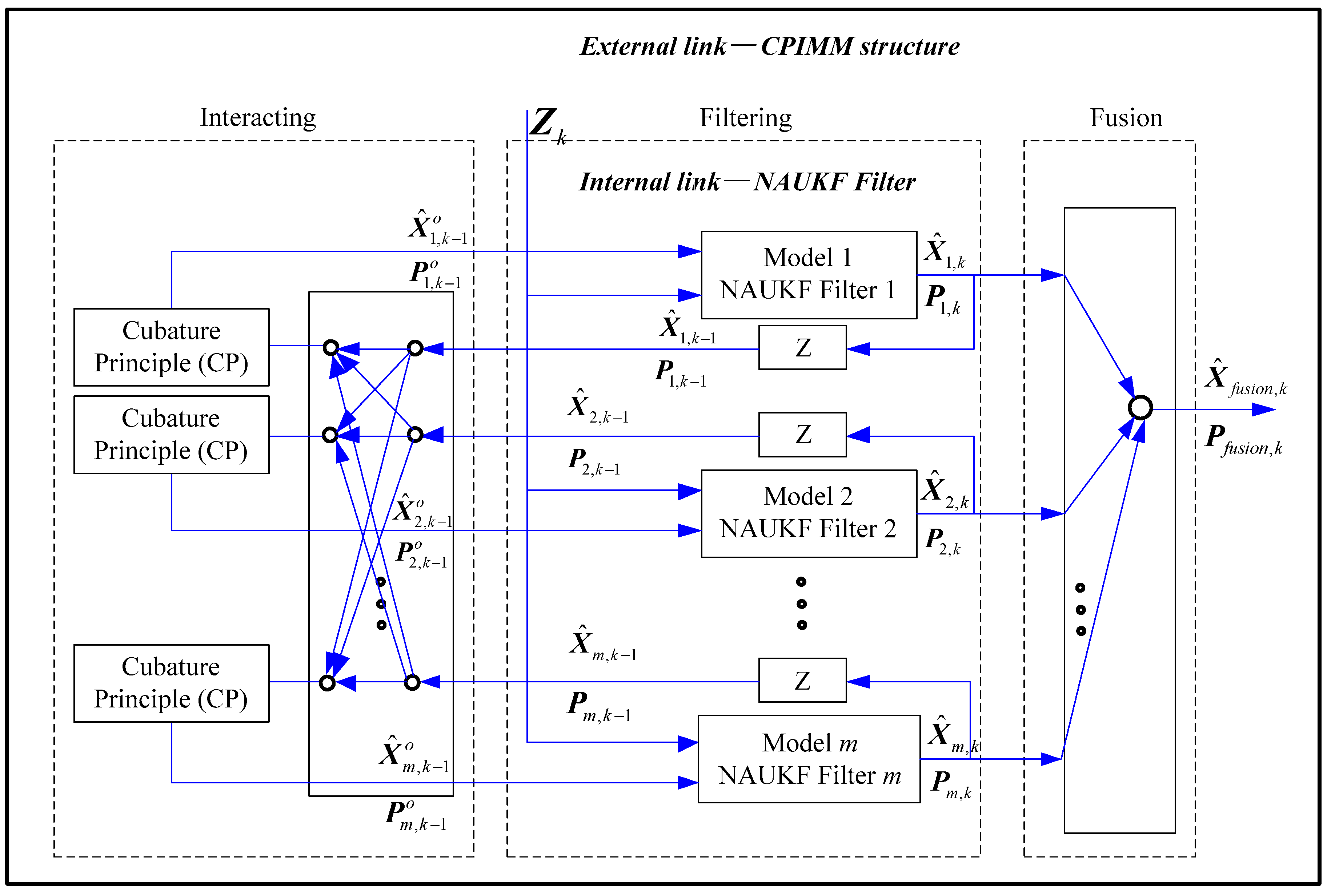
Figure 4.
True trajectory of the maneuvering target.
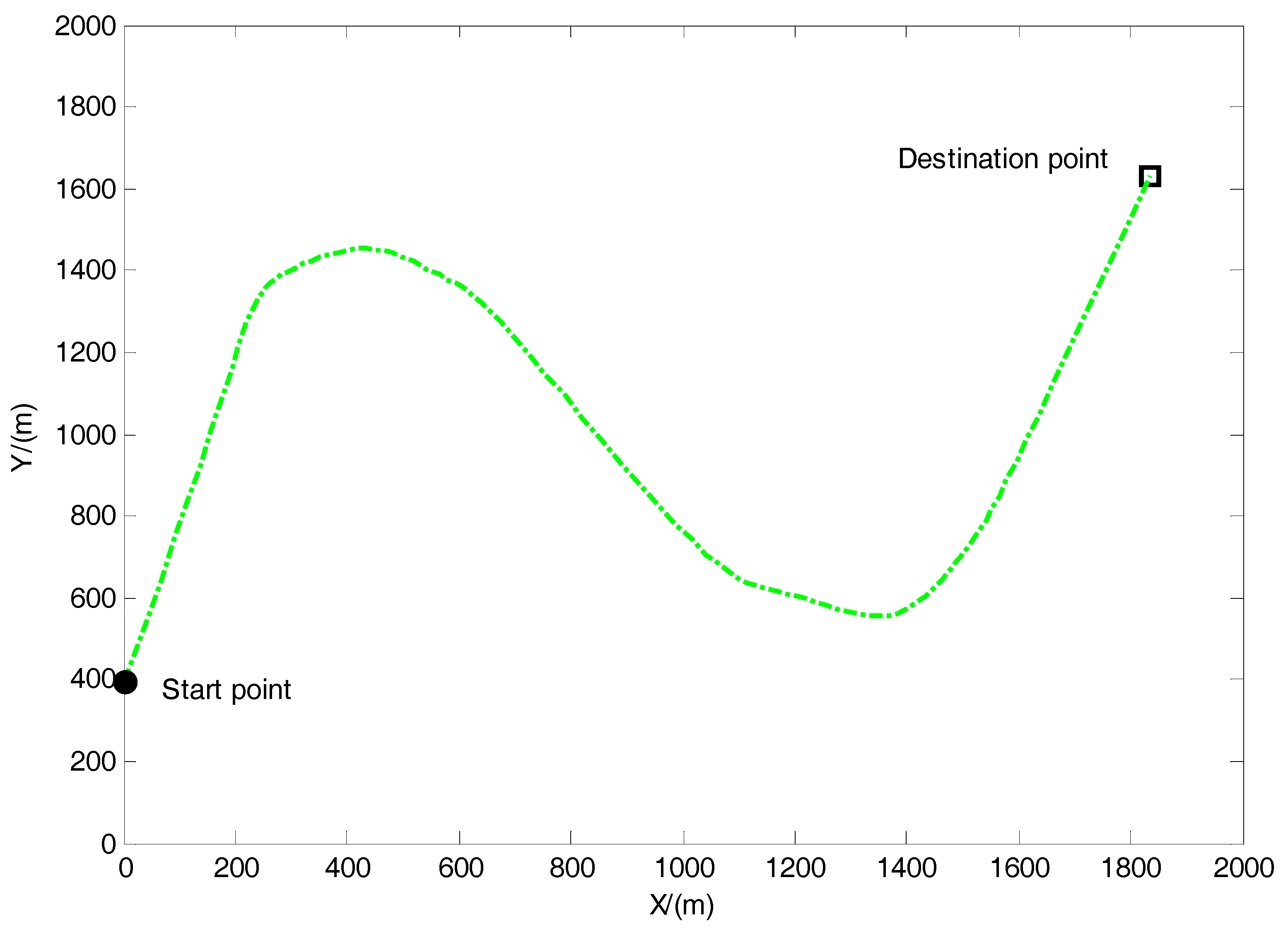
Figure 5.
True and estimated trajectories of the maneuvering target for CPIMM for Case 1.

Figure 6.
Position root mean square error (RMSE) comparison for CPIMM for Case 1.
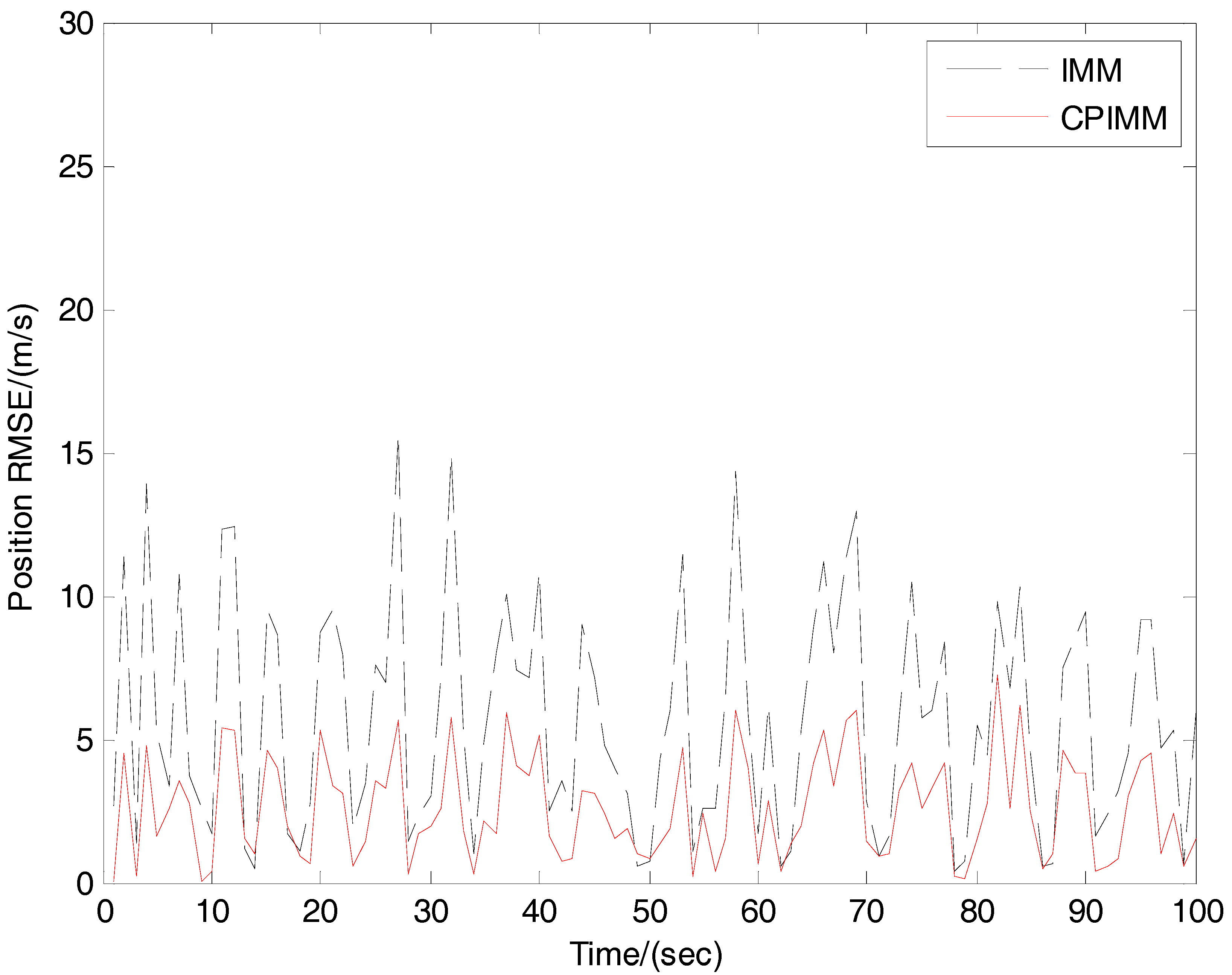
Figure 7.
Velocity RMSE comparison for CPIMM for Case 1.
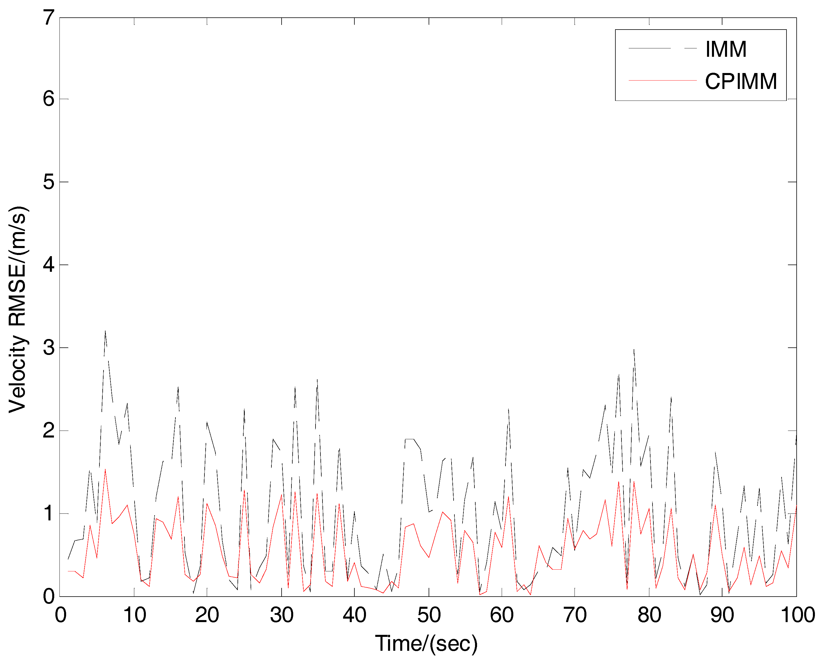
Figure 8.
True and estimated trajectories of the maneuvering target for CPIMM-NAUKF for Case 2.
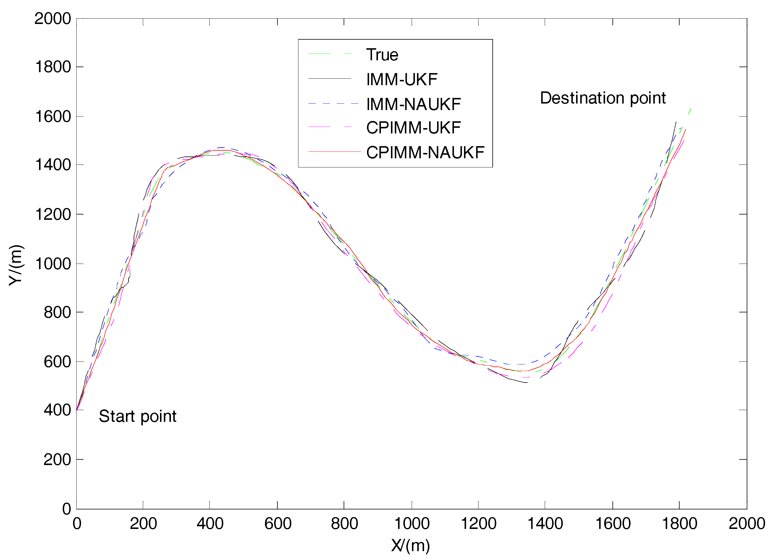
Figure 9.
Position RMSE comparison for CPIMM-NAUKF for Case 2.
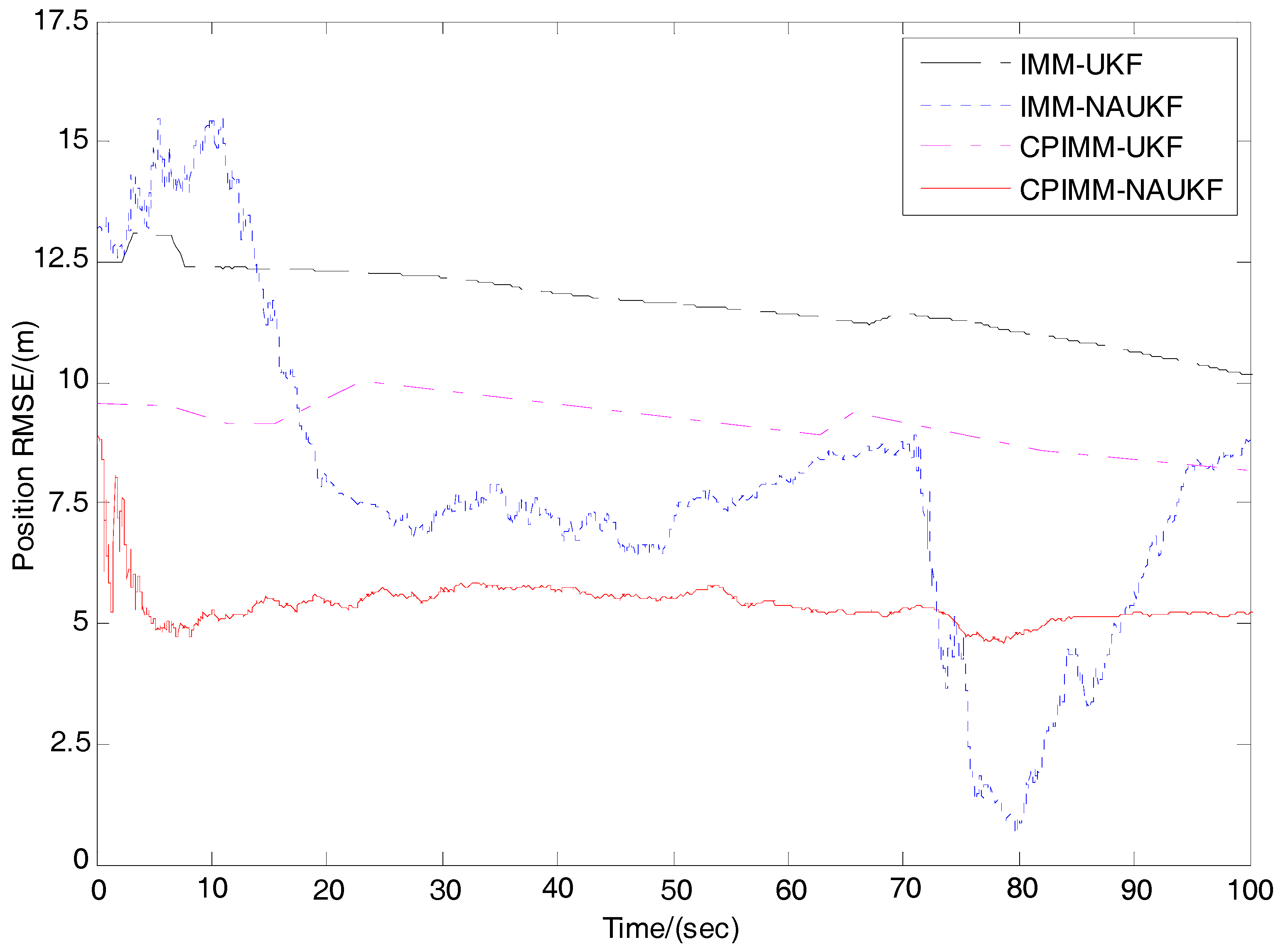
Figure 10.
Velocity RMSE comparison for CPIMM-NAUKF for Case 2.

Figure 11.
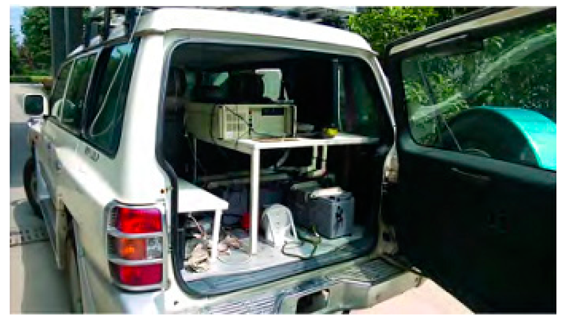
The experimental vehicle.

Figure 12.
The vehicle loaded navigation equipment.

Figure 13.
The real route of the vehicle in navigation.
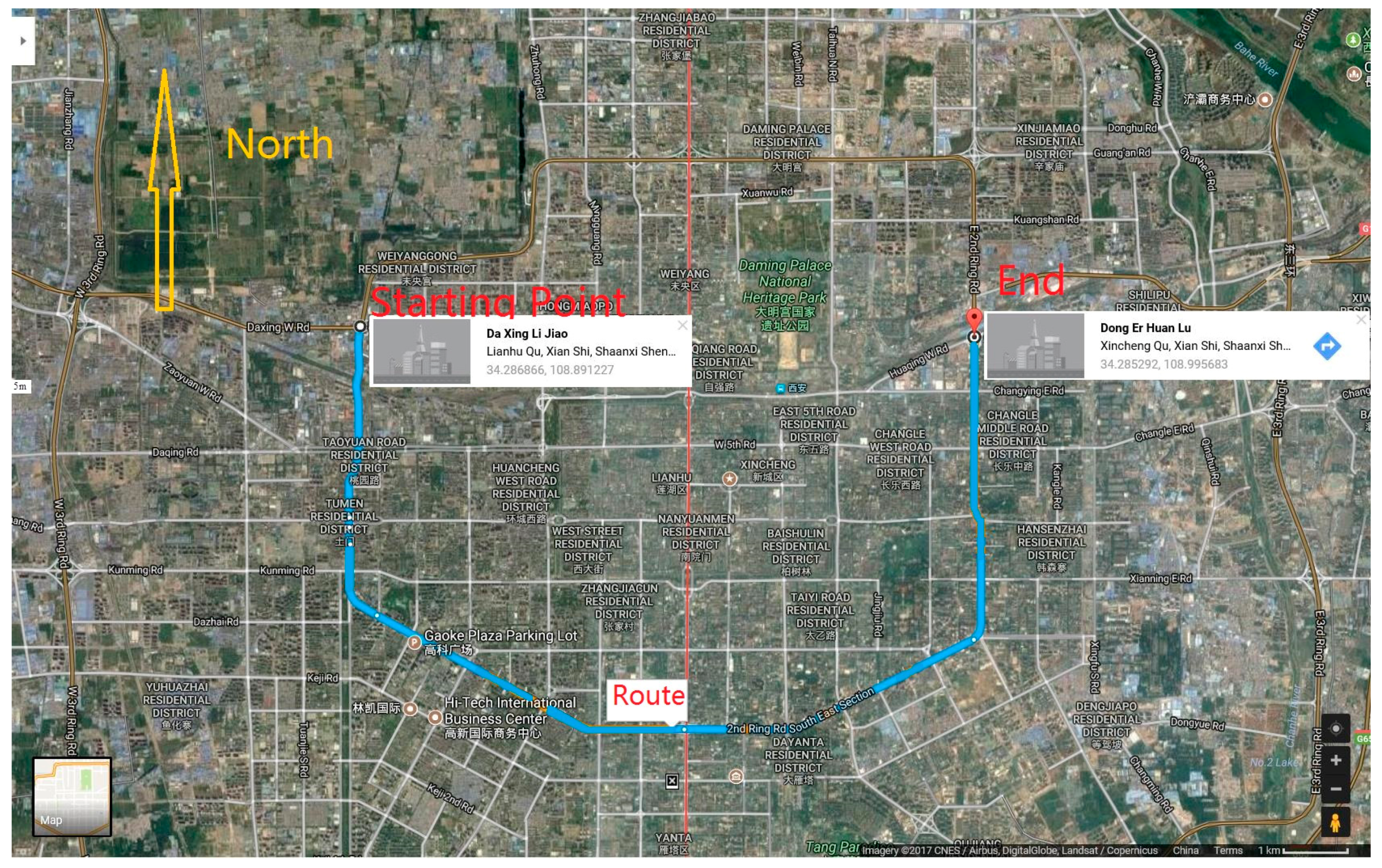
Figure 14.
Longitude error comparison for NAUKF in INS/GPS navigation system.

Figure 15.
Latitude error comparison for NAUKF in INS/GPS navigation system.

Figure 16.
The experimental unmanned aerial vehicle (UAV).
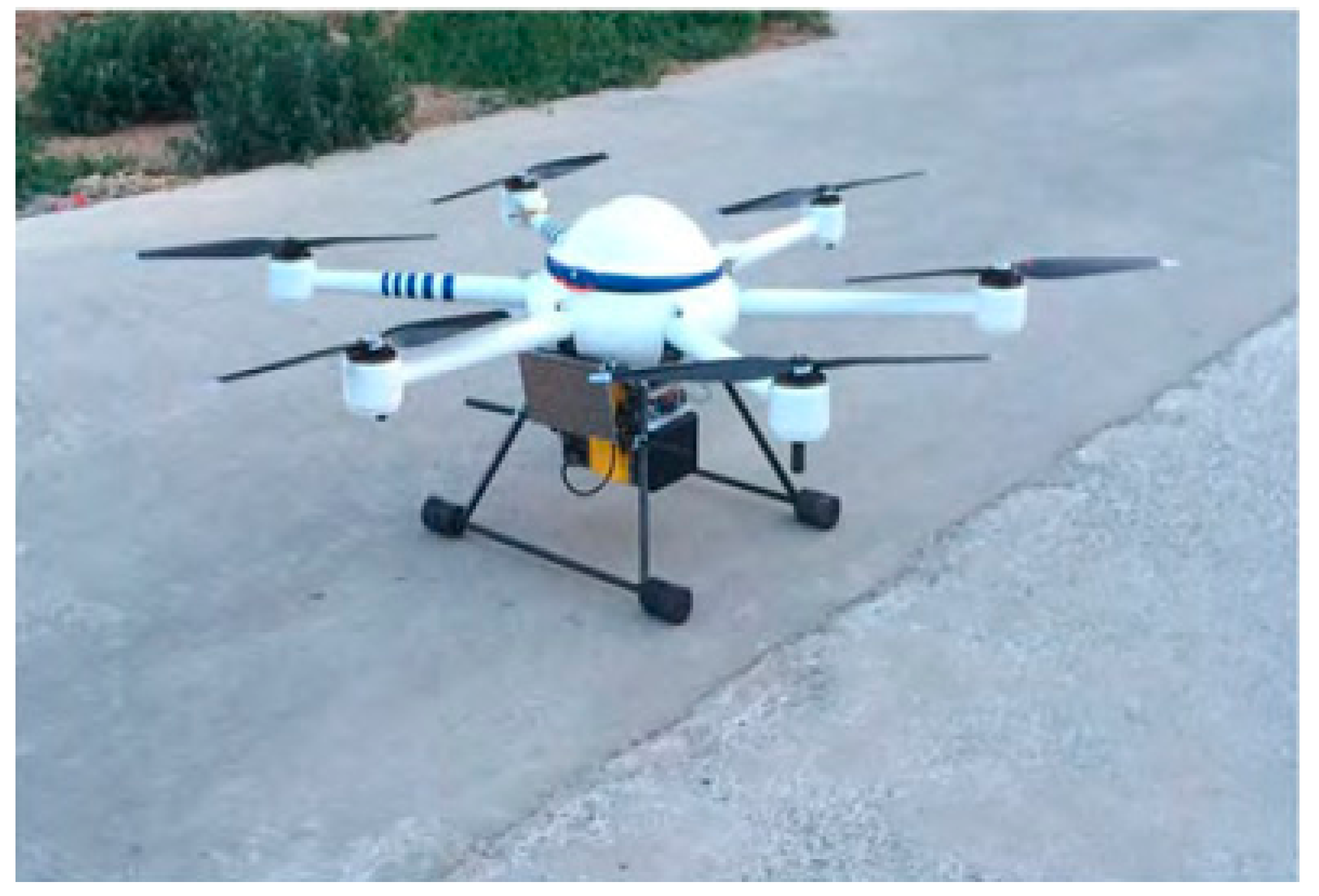
Figure 17.
The UAV loaded tracking equipment; (a): SAR (synthetic aperture radar); (b): Antenna.
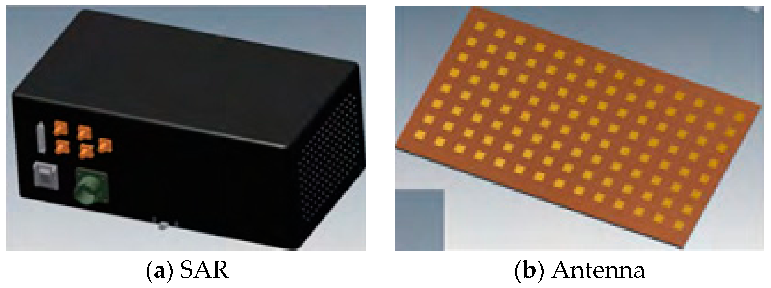
Figure 18.
The real route of the vehicle in target tracking.
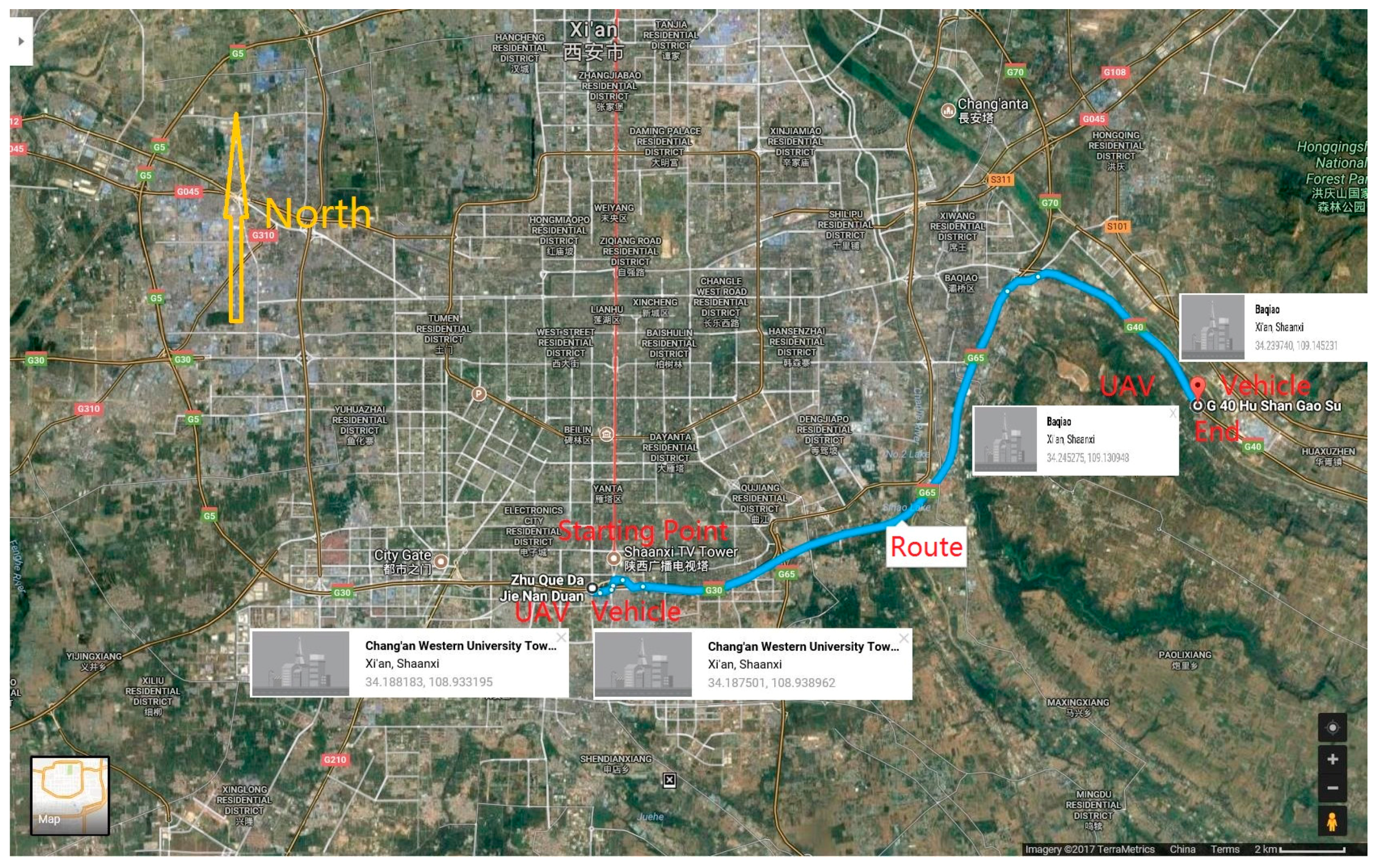
Figure 19.
Longitude error comparison for CPIMM-NAUKF in SAR tracking system.

Figure 20.
Latitude error comparison for CPIMM-NAUKF in the synthetic aperture radar (SAR) tracking system.
Figure 20.
Latitude error comparison for CPIMM-NAUKF in the synthetic aperture radar (SAR) tracking system.


Table 1.
Calculation results of the comparison of the mean and covariance matrix after interaction; MSE: the mean square error; MC: Monte Carlo.
Table 1.
Calculation results of the comparison of the mean and covariance matrix after interaction; MSE: the mean square error; MC: Monte Carlo.
| Method | Mean | Covariance |
|---|---|---|
| MSE | 0.6000 | 3.9417 |
| MC | 0.5937 | 1.3906 |
Table 2.
Performance comparison of the algorithms for CPIMM for Case 1.
| Algorithm | Position Error (m) | Velocity Error (m/s) | ||
|---|---|---|---|---|
| Mean | Standard Deviation | Mean | Standard Deviation | |
| IMM | 3.8245 | 2.0377 | 0.7102 | 0.6935 |
| CPIMM | 2.0630 | 1.1604 | 0.4596 | 0.4187 |
Table 3.
Performance comparison for CPIMM-NAUKF for Case 2.
| Algorithm | Position Error (m) | Velocity Error (m/s) | ||
|---|---|---|---|---|
| Mean | Standard Deviation | Mean | Standard Deviation | |
| IMM-UKF | 11.8533 | 4.3387 | 3.1026 | 1.9552 |
| IMM-NAUKF | 7.0473 | 2.9116 | 1.2143 | 1.0348 |
| CPIMM-UKF | 9.3558 | 3.0098 | 2.4961 | 1.2246 |
| CPIMM-NAUKF | 4.8671 | 0.9169 | 0.4294 | 0.3857 |
Table 4.
Performance comparison for NAUKF in INS/GPS navigation system.
| Algorithm | Mean Absolute Error of Longitude (m) | Mean Absolute Error of Latitude (m) | ||
|---|---|---|---|---|
| Mean | Standard Deviation | Mean | Standard Deviation | |
| EKF | 8.6533 | 7.9816 | 8.2107 | 7.0044 |
| CKF | 8.4154 | 7.5127 | 8.0109 | 6.8135 |
| UKF | 6.9018 | 6.5011 | 6.9271 | 6.6102 |
| AUKF | 4.4225 | 4.0118 | 4.8159 | 4.6825 |
| NAUKF | 3.0156 | 2.8105 | 2.8192 | 2.4947 |
Table 5.
Performance comparison for CPIMM-NAUKF in the SAR tracking system.
| Algorithm | Mean Absolute Error of Longitude (m) | Mean Absolute Error of Latitude (m) | ||
|---|---|---|---|---|
| Mean | Standard Deviation | Mean | Standard Deviation | |
| IMM-UKF | 9.0125 | 8.2336 | 9.0058 | 8.1329 |
| IMM-NAUKF | 6.7243 | 6.0772 | 6.1174 | 5.9287 |
| CPIMM-UKF | 7.1588 | 7.0154 | 7.0542 | 6.8835 |
| CPIMM-NAUKF | 2.8514 | 2.2259 | 2.3417 | 2.0016 |
© 2017 by the authors. Licensee MDPI, Basel, Switzerland. This article is an open access article distributed under the terms and conditions of the Creative Commons Attribution (CC BY) license (http://creativecommons.org/licenses/by/4.0/).
Share and Cite
MDPI and ACS Style
Zhou, H.; Zhao, H.; Huang, H.; Zhao, X. A Cubature-Principle-Assisted IMM-Adaptive UKF Algorithm for Maneuvering Target Tracking Caused by Sensor Faults. Appl. Sci. 2017, 7, 1003. https://doi.org/10.3390/app7101003
AMA Style
Zhou H, Zhao H, Huang H, Zhao X. A Cubature-Principle-Assisted IMM-Adaptive UKF Algorithm for Maneuvering Target Tracking Caused by Sensor Faults. Applied Sciences. 2017; 7(10):1003. https://doi.org/10.3390/app7101003
Chicago/Turabian StyleZhou, Huan, Hui Zhao, Hanqiao Huang, and Xin Zhao. 2017. "A Cubature-Principle-Assisted IMM-Adaptive UKF Algorithm for Maneuvering Target Tracking Caused by Sensor Faults" Applied Sciences 7, no. 10: 1003. https://doi.org/10.3390/app7101003
Note that from the first issue of 2016, this journal uses article numbers instead of page numbers. See further details here.