A Rolling Bearing Fault Diagnosis Method Based on Variational Mode Decomposition and an Improved Kernel Extreme Learning Machine


1
Jiangsu Key Laboratory of Advanced Food Manufacturing Equipment and Technology, Jiangnan University, 1800 Li Hu Avenue, Wuxi 214122, Jiangsu, China
2
School of Mechanical and Electrical Engineering, Beijing University of Chemical Technology, 15 Beisanhuan East Road, ChaoYang District, Beijing 100029, China
3
Graduate School of Bioresources, Mie University, 1577 Kurimamachiya-cho, Tsu, Mie 514-8507, Japan
*
Authors to whom correspondence should be addressed.
Appl. Sci. 2017, 7(10), 1004; https://doi.org/10.3390/app7101004
Submission received: 2 August 2017
/
Accepted: 19 September 2017
/
Published: 29 September 2017
(This article belongs to the Section Mechanical Engineering)
Abstract
:Rolling bearings are key components of rotary machines. To ensure early effective fault diagnosis for bearings, a new rolling bearing fault diagnosis method based on variational mode decomposition (VMD) and an improved kernel extreme learning machine (KELM) is proposed in this paper. A fault signal is decomposed via VMD to obtain the intrinsic mode function (IMF) components, and the approximate entropy (ApEn) of the IMF component containing the main fault information is calculated. An eigenvector is created from the approximate entropy of each component. A bearing diagnosis model is created via a KELM; the KELM parameters are optimized using the particle swarm optimization (PSO) algorithm to obtain a KELM diagnosis model with optimal parameters. Finally, the effectiveness of the diagnosis method proposed in this paper is verified via a fan bearing fault diagnosis test. Under identical conditions, the result is compared with the results obtained using a back propagation (BP) neural network, a conventional extreme learning machine (ELM), and a support vector machine (SVM). The test result shows that the method proposed in this paper is superior to the other three methods in terms of diagnostic accuracy.
1. Introduction
Rolling bearings are critical components that are widely deployed in rotary machines, and their operational state directly affects a device’s performance, operational efficiency, and lifetime. If the root cause of a fault could be traced in the early stage of the fault’s development to eliminate hidden risk and prevent serious accidents, it would have significant economic and practical value [1,2]. In actual engineering projects, the features of bearing faults in the early stages of fault development are inconspicuous. Additionally, vibration transmission path attenuation and background noise interference severely hinder the extraction of fault features. Therefore, the question of how to effectively eliminate noise and extract valid fault features is the key to rolling bearing monitoring and state identification.
As a powerful non-linear, non-stationary signal processing tool, empirical mode decomposition (EMD) [3] immediately caught the attention of researchers in the area of machine fault diagnosis once it was proposed. Based on a gray association model, Wang et al. [4] created a mapping between the intrinsic mode function (IMF) energy distribution and bearing state for bearing state identification. In reference [5], a support vector machine (SVM) and EMD were combined for diagnosis of a rolling bearing’s fault envelop spectrum. Ali et al. [6] combined EMD and a neural network for bearing fault diagnosis. Inspired by EMD, Smith proposed another adaptive signal decomposition method, local mean decomposition (LMD), in 2005 [7]; this method also attracted significant attention from researchers, and numerous LMD-based diagnosis methods were proposed in succession. Chen et al. [8] employed LMD for rolling bearing and gear fault diagnosis. Liu et al. [9] obtained a wind power generator’s vibration signal instantaneous frequency via LMD to monitor the wind power generator’s state. EMD and LMD have been widely deployed to extract fault features. However, the two methods belong to recursive mode decomposition, which is affected by mode aliasing, end effects, and sampling frequency. When the frequency ratio is the reciprocal of an odd number, the decomposition has significant error [10].
Variational mode decomposition (VMD) is a new adaptive signal processing method proposed by Dragomiretskiy and Zosso [11]. VMD assumes that each intrinsic mode function has limited bandwidth and a different central frequency. To ensure the sum of the estimated bandwidths for the intrinsic mode functions is minimal, a variation problem is solved via a transformation. Each intrinsic mode function is demodulated to the corresponding base frequency band. Finally, each intrinsic mode function and its corresponding central frequency are extracted. Once VMD was proposed, it immediately became the focus of fault diagnosis research. Aneesh et al. [12] analyzed and compared the feature extraction performance of VMD and the empirical wavelet transform, and suggested that VMD was superior for feature extraction. Mohanty et al. [13] applied VMD to bearing fault diagnosis. Lv, et al. [14] decomposed a vibration signal via VMD and employed an immunogenic algorithm-optimized support vector machine for fault identification.
Artificial neural networks (ANN) have been widely deployed in fault diagnosis. However, conventional neural networks employ learning algorithms based on gradient descent and have problems such as slow convergence and being trapped in local minima. Extreme learning machine (ELM) is a recently proposed single-hidden-layer forward neural network learning algorithm [15]. In ELM, the input weight of the input layer and threshold of the hidden layer node are selected randomly, and the output weight is calculated via the Moore–Penrose generalized inverse of the hidden layer’s output matrix. Compared with conventional neural networks, ELM has advantages such as a fast learning speed and excellent generalization performance. However, the randomly generated hidden layer weight and hidden layer threshold have significant impacts on the ELM algorithm’s performance. SVM is a powerful tool for problems with a small sample, and has high computational efficiency and good generalization ability. SVM has been applied in the fault diagnosis of rolling bearings [16], wind turbines [17], motor rotors [18], and air compressors [19]. However, SVM is a binary classifier algorithm, which has the disadvantage of classification model building difficulty and low classification efficiency in multi-classification problems. In addition, the optimal classification surface of SVM is determined by the support vector at the edge of the class, and the traditional SVM is particularly sensitive to noise and outliers in the training samples. These problems reduce the diagnostic performance of SVM. Kernel extreme learning machine (KELM) is an improved algorithm proposed by Huang [20] based on the ELM algorithm and a kernel function. KELM not only possesses numerous advantages of the ELM algorithm, but also integrates a kernel function and maps linearly inseparable modes into a high-dimensional feature space to make them linearly separable; therefore, the identification accuracy is improved. KELM does not require its user to determine the number of hidden layer nodes in advance. Compared with ELM, in the network training and learning stages, KELM only requires its user to select the proper kernel parameters and the normalization coefficient to obtain the network output weight via matrix calculations. In reference [21], a multi-kernel extreme learning machine method was proposed and applied to multi-element chaotic time series forecasts to obtain accurate forecasts. In reference [22], a fast single-winner cross validation online KELM method was proposed and successfully applied in chaotic time series forecasts and process recognition for continuously stirred tank reactors. However, the kernel function makes the KELM algorithm sensitive to parameter setting. Therefore, optimal parameter selection is the key to improving the KELM method’s state forecast accuracy.
For the above problems, a bearing fault diagnosis method based on VMD and an improved KELM algorithm is proposed in this paper. First, the fault signal is decomposed via VMD to obtain the IMF components. Next, the approximate entropy of the IMF component containing major fault information is calculated, and an eigenvector is created from the approximate entropy of each component. Then, the KELM parameters are optimized via the particle swarm optimization (PSO) algorithm to obtain a KELM with optimal parameters. Finally, the method proposed in this paper is applied to bearing fault diagnosis to verify its effectiveness.
2. Variational Mode Decomposition
VMD is a solution process for variation problems based on classical Weiner filtering, Hilbert transformation, and frequency mixture. Adaptive signal decomposition is implemented by identifying the optimal solution of the constrained variation model. The input signal is decomposed into multiple sparse mode components.
Assume that each mode has limited bandwidth with a central frequency; the central frequency and bandwidth are updated continuously during the decomposition. VMD is to identify the mode function with the minimum sum of the K estimated bandwidths; the sum of the modes is the input signal .
- (1)
- Each mode function undergoes a Hilbert transformation to obtain the analytical signal of each intrinsic mode function and the unilateral frequency spectrum:
- (2)
- The estimated central frequencies of all the analytical mode signals are merged, and the corresponding mode frequency spectrum is modulated in the respective base frequency band:
- (3)
- The square norm of the gradient of the demodulated signal is calculated, and the bandwidth of each mode component is estimated. The expression for the corresponding constrained variation model is as follows:where represents the K IMF components after decomposition, , and represents central frequency of each component, .
The second-order penalty factor and Lagrange multiplying operator are introduced. The second-order penalty factor guarantees signal reconfiguration accuracy in environments with Gaussian noise. The Lagrange operator ensures the strictness of the constrained condition. The extended Lagrange expression is as follows:
where, α is the penalty factor and λ(t) is the Lagrange operator.
The “saddle point” of extended Lagrange expression is calculated via the alternating direction method of multiplier (ADMM) algorithm. The detailed procedure is as follows:
- (1)
- Initialize ;
- (2)
- Execution cycle: ;
- (3)
- For all , update :
- (4)
- Update :
- (5)
- Update :
- (6)
- Repeat steps (2) through (5) until the iteration stop condition is satisfied:
- (7)
- Stop iteration and obtain the K IMF components.
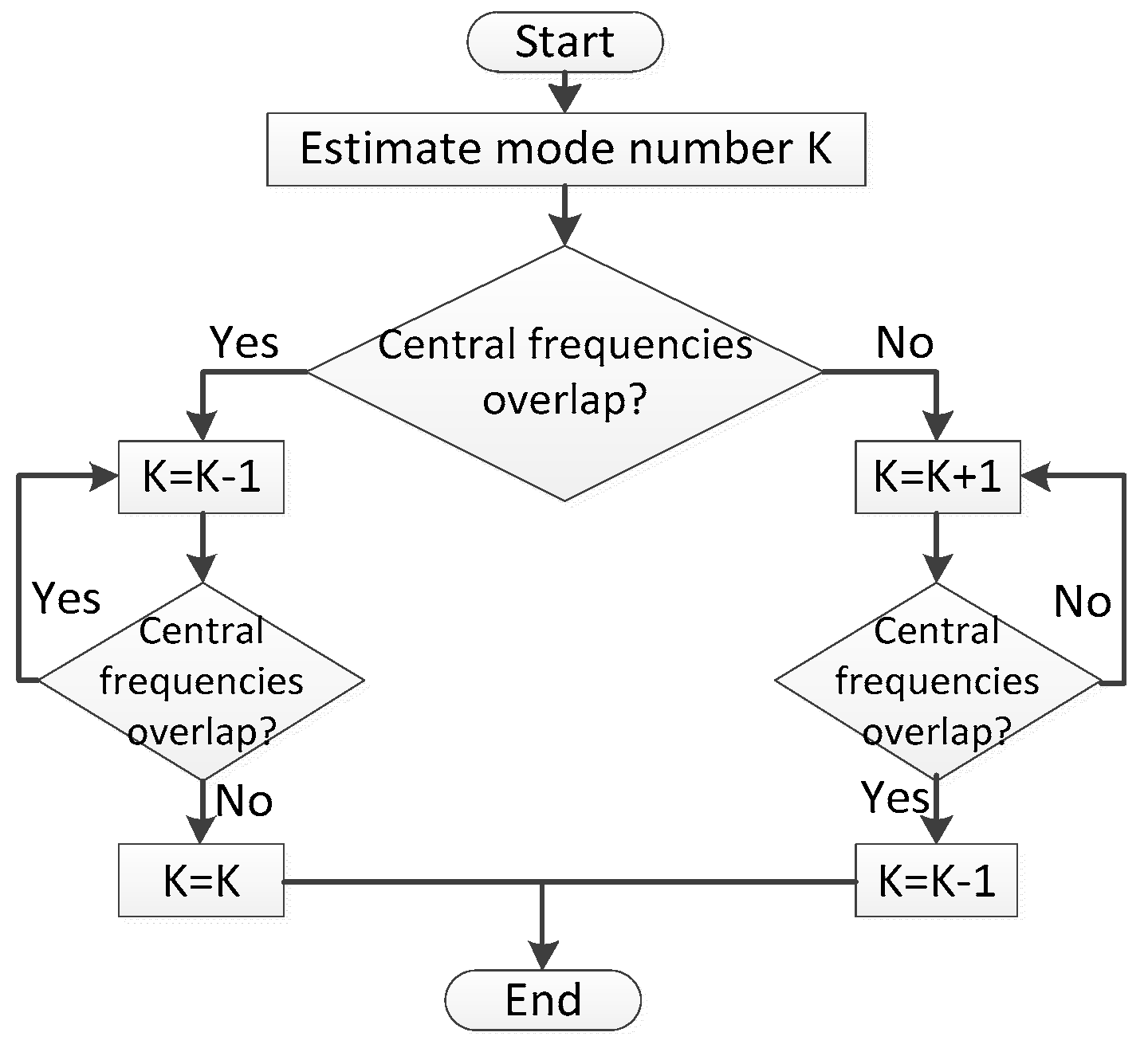
Before VMD, the number of modes K should be determined. If K is too small, multiple components of the signal may be contained in one mode simultaneously, or one component may not be able to be estimated. If K is too large, one component in the signal could be included in multiple modes, and the mode central frequencies obtained by iteration will eventually overlap. To address this problem, a mode number fluctuation method is proposed in this paper to determine the mode number K. The detailed procedure is as follows, and the flowchart is shown in Figure 1.
- (1)
- The initial value of the mode number is K = K0;
- (2)
- When the mode number is K0, determine whether the mode central frequencies overlap;
- (3)
- If the central frequencies overlap, decrease the mode number and perform VMD until the central frequencies do not overlap. Return K;
- (4)
- If the central frequencies do not overlap, increase the mode number and perform VMD until the central frequencies overlap. Return K − 1.
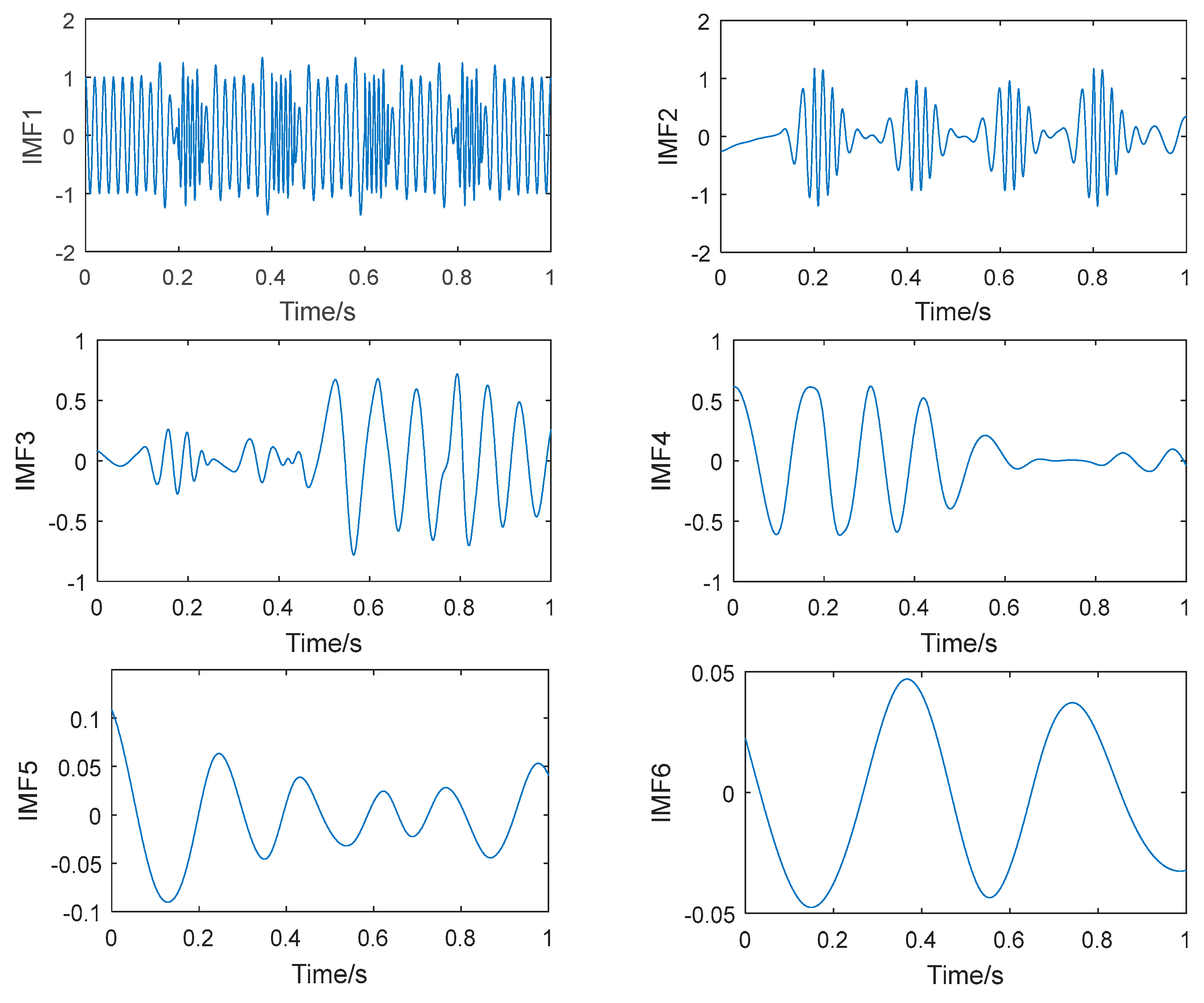
A simulation test is designed to verify the effectiveness of VMD. Simulation signal y(t) consists of interval signal x1(t), linear frequency modulation signal x2(t), and cosine signal x3(t); the time domain waveform is shown in Figure 2. The simulation signal is decomposed via the VMD, EMD, and LMD methods, as shown in Figure 3, Figure 4 and Figure 5. The decomposition result shows that the VMD method decomposes various signal components effectively and the decomposed signal and original signal have a high degree of coincidence. In comparison, the EMD- and LMD-processed intrinsic modes have various degrees of mode aliasing and signal distortion. The main reasons are considered as follows: both the EMD and LMD algorithms define local mean functions and local envelope functions based on extreme points (maxima and minima), and their envelope estimation errors will be amplified after repeated recursive decomposition. Therefore, the EMD and LMD algorithms are very sensitive to noise. When the decomposed signal contains interval or adjacent frequency components, modal aliasing often occurs in the EMD and LMD algorithms, and the adjacent frequency components are hard to decompose. In addition, due to the effect of end effects, the signal contains some false components, resulting in demodulation errors. In the simulation signal y(t), the frequencies of x1(t) and x2(t) are 5 Hz and 10 Hz, respectively, with adjacent frequency components. In addition, y(t) also contains interval signal components. Therefore, the simulation signal y(t) cannot be effectively decomposed by using the EMD and LMD algorithms. VMD assumes that each intrinsic mode function has limited bandwidth and a different central frequency. To ensure that the sum of the estimated bandwidths for the intrinsic mode functions is minimal, a variation problem is solved via a transformation. Each intrinsic mode function is demodulated to the corresponding base frequency band. Finally, each intrinsic mode function and its corresponding central frequency are extracted. VMD is an adaptive Wiener filter group, which shows better noise robustness. Therefore, VMD effectively solves the mode aliasing problem and has significantly superior anti-noise performance compared with EMD and LMD. Additionally, because the VMD algorithm is applied in the frequency domain and belongs to a complete non-recursive algorithm, it has higher computational efficiency than EMD and LMD.
3. Approximate Entropy
In the field of fault diagnosis, many symptom parameters (SPs) have been defined to reflect the features of vibration signals measured for condition diagnosis, such as root mean square (RMS), skewness, and kurtosis,. In this study, the approximate entropy (ApEn) calculated from four IMF components is used to extract the vibration signal feature of each bearing state. ApEn is a physical quantity that measures the probability of generating a new mode in a signal to reflect the complexity of a time series. It only requires a short series of data, has superior anti-noise capability, and is applicable to both random and deterministic signals [23].
Assume that the original data are , and denote the mode dimension and similarity tolerance as m and r, respectively. Normally, the ApEn is calculated via the following procedure:
- Based on the series , the dimension is expanded in sequence to an -dimensional vector :
- The distance between each and other vectors is calculated:
- Assume that the threshold is . For each , the number of is counted, and the ratio of this number to the total number of vectors is calculated as follows:
- The logarithm of is calculated, and the average of all is denoted as :
- The above procedure is repeated to obtain . Then, theoretically, the ApEn is computed as follows:
The above final value is normally represented as having probability 1. However, cannot approach ∞. Therefore, the result calculated via the above procedure is actually an estimate of the ApEn for a series with length , denoted as
The above expression shows that ApEn is related to m and r. Normally, when ( is the standard deviation of the series ), the statistical characteristics of ApEn are more reasonable.
4. Improved Kernel Extreme Learning Machine
4.1. Brief Outline of KELM
Assume that are the original data, is the corresponding target output, is the target output set, the number of hidden layer neurons is , is the weight of the connection between the i-th hidden layer neuron and the output layer, and is the activation function that maps data from the input layer to the i-th hidden layer neuron. Then, the ELM output is as follows:
The ELM training goal is defined as follows:
where the first part of is the structural risk, and the second part is the empirical risk; is a penalty coefficient; is the theoretical output; and is the error of versus .
To solve the above optimization problem, a Lagrange function is defined as follows, where is a Lagrange factor:
Based on Karush–Kuhn–Tucker (KKT) theory, the solution for the above equation is as follows:
It follows that
where T = [t1, t2 ····· tN]T is the target vector of the input sample.
The hidden layer output matrix consists of randomly generated weights of connections between the input layer and hidden layer and thresholds of hidden layer neurons. In essence, it is a random mapping. Owing to such randomness, a different is generated each time. Therefore, the calculated is different, which leads to fluctuations in the ELM output and inferior stability and generalization capability [24]. Huang et al. replaced with a kernel function to obtain the KELM algorithm, which prevents random assignment-induced fluctuations in the results of KLM:
Equations (24) and (25) are substituted into Equation (18) to obtain the KELM output:
A radial basis function (RBF) is used as the kernel function:
4.2. KELM Optimized Using PSO
When implementing the KELM learning algorithm, the parameters C and σ have significant impacts on the algorithm’s performance. The PSO algorithm [25] is a random search and parallel optimization algorithm that has advantages such as simplicity, ease of implementation, and quick convergence. Therefore, in this paper, C and σ are optimized using the PSO algorithm to create a PSO-optimized KELM forecast model. When implementing the PSO-KELM method, the method for optimal parameter selection for KELM is an optimization of the penalty coefficients C and kernel function parameter σ. The KELM classification accuracy is defined as acc (C, σ). In the KELM parameter optimization model, the maximum classification accuracy for the PSO fitness function is given by Equation (27). That is, a set of C and σ are identified within a given range to ensure the maximum classification accuracy for the KELM classifier.
The detailed modeling procedure of the PSO-KELM diagnosis model is as follows:
- (1)
- A particle swarm is generated based on the number of groups. The position and velocity of each particle are randomly initialized.
- (2)
- F is calculated via Equation (28) as the individual fitness to determine the optimal position of individual particle ; the optimal position for each group is .
- (3)
- The particle velocity and position are updated using following equations:
- (4)
- Steps (2) and (3) are repeated until the termination condition is satisfied. The optimal parameters C and σ are returned.
5. Test and Verification
5.1. Test Platform
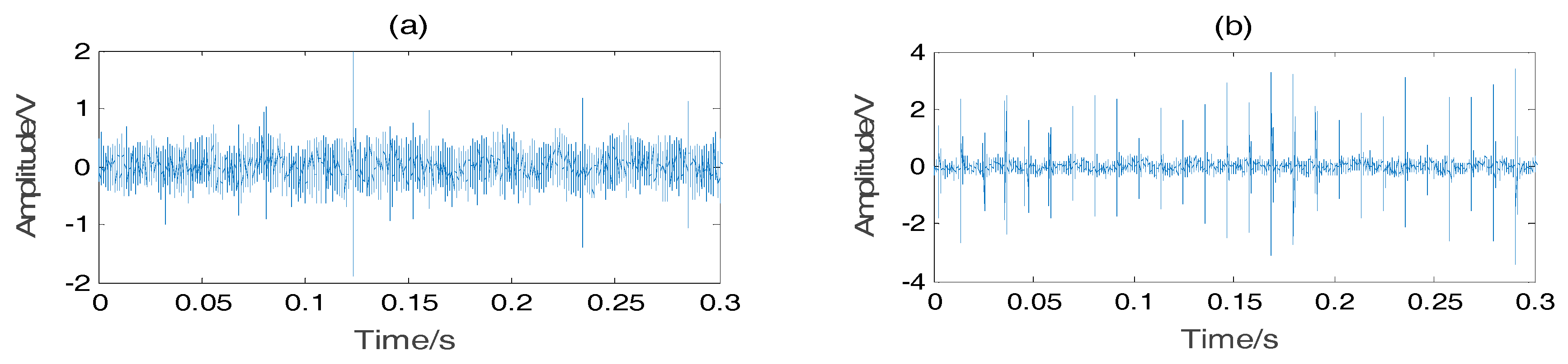
To verify the effectiveness of the method presented in this paper for the analysis of vibration signals from actual measurements, a rolling bearing fault signal of a centrifugal fan is analyzed. Figure 6 shows the centrifugal fan test platform used in this test. Based on a rolling bearing fault in an actual engineering project, a wire-cutting machine is employed to produce tiny dents in the rolling bearing’s outer ring, inner ring, and roller in the fan test bed to simulate early stage faults and defects in the outer ring, inner ring, and roller. Details are shown in Figure 7. A PCB MA352A60 accelerometer (PCB MA352A60, PCB Piezotronics Inc., New York, NY, USA) is fixed at the top of the bearing pedestal via a screw to collect vibration signal data in the vertical direction, including the rolling bearing’s normal vibration signal and fault signals of the outer ring, inner ring, and roller. The signals are amplified via a sensor signal regulator (PCB ICP Model 480C02, PCB Piezotronics Inc., New York, NY, USA) and transmitted to a signal recorder (Scope Coder DL750,Yokogawa Co. Ltd., Tokyo, Japan). In the test, the rotation speed is set to 1000 rpm, the sampling frequency fs is 50 kHz, and the sampling duration is 10 s. The size of the data collected is 2,000,000, and the data length of each state is 500,000. Figure 8 shows the original vibration signal in each state. The bearings that are utilized, the specifications of the test bearing, the size of the faults, and other necessary information are listed in Table 1.
5.2. Condition Detection via the Proposed Method
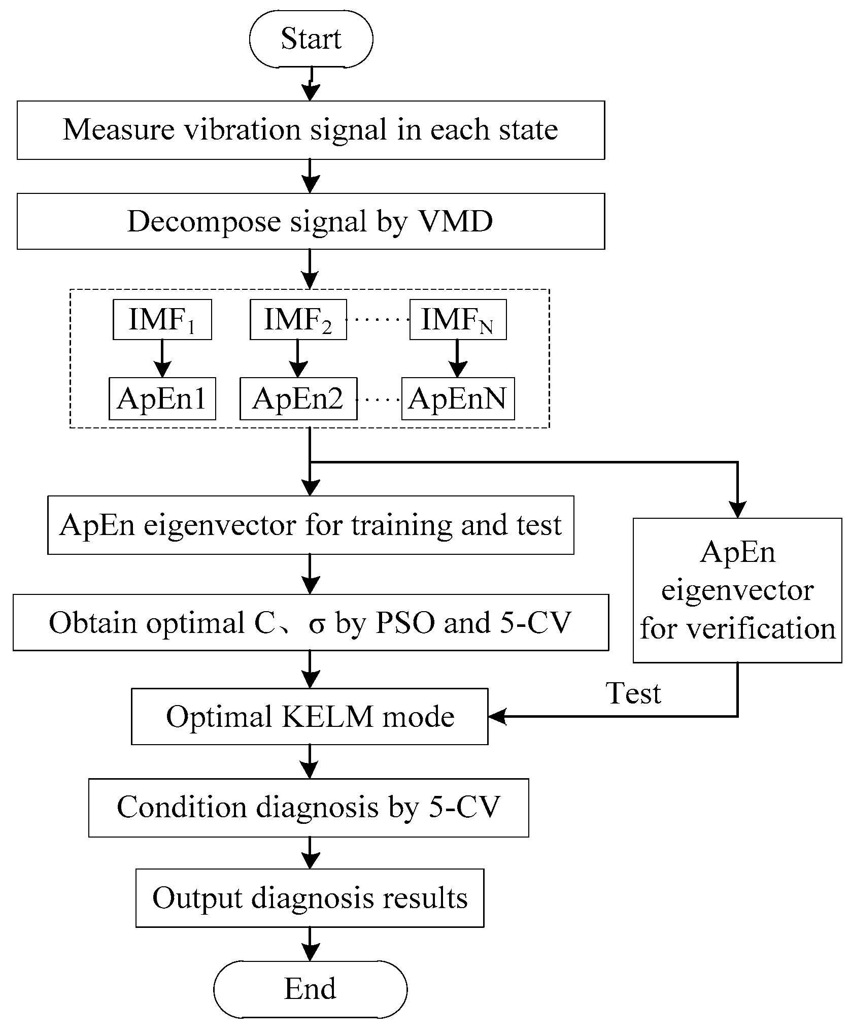
Figure 9 shows the procedure of the fault diagnosis method proposed in this paper. First, the vibration signal is decomposed via the VMD method introduced in Section 2. Figure 10, Figure 11, Figure 12 and Figure 13 show the decomposition results of the collected vibration signals of the bearing in each state. Each state has four corresponding decomposed IMF components, and 300 ApEn values are calculated for each IMF. An eigenvector is created from the ApEn of each component.
To explain the efficiency of ApEn, we compare the sensitivity of ApEn with RMS, skewness, and kurtosis by the detection index method (DI) [26].
Suppose that x1 and x2 are the SP values calculated from the signals measured in state 1 and state 2, respectively, and their average and standard deviation are μ and σ. The DI is calculated by
The Distinction Rate (DR) is defined as
It is obvious that the larger the value of the DI, the larger the value of the DR will be, and therefore, the better the SP will be. Thus, the DI can be used as the index of quality to evaluate the distinguishing sensitivity of the SP.
Table 2 lists the DI values of each SP. The distribution information of the ApEn is shown in Table 3. From Table 2, the DI values of ApEn are higher than RMS, skewness, and kurtosis; that is to say, the sensitivity of ApEn for bearing diagnosis is higher than that of other SPs.
The KELM parameters are optimized via the PSO algorithm to obtain the KELM training model with optimal parameters. The process of KELM model training and optimization of the parameters C and σ is shown in Figure 14. Assume that a particle swarm contains 50 particles, the acceleration factors η1 and η2 are 2, and the maximum number of iterations is 1000. In order to minimize possible effects of data outliers, a fivefold cross validation method (5-CV) is adopted for parameter optimization and condition identification. The calculated ApEn sample is randomly partitioned into five subsamples. Of the five subsamples, three subsamples are retained as the training data, one subsample is used as test data for parameter optimization, and the remaining one subsample is used as verification data for condition identification of the bearing. As an example, some PSO-KELM training data are listed in Table 4.
After parameter optimization, the bearing condition identification is performed by the optimal KELM and 5-CV method. The verification result shown in Table 5 demonstrates that the normal state average diagnosis accuracy reaches 100%, the outer ring defect state average fault diagnosis accuracy reaches 90.3%, the outer ring defect state average fault diagnosis accuracy reaches 85.7%, the roller element defect state average fault diagnosis accuracy reaches 96.3%, and the overall accuracy reaches 93.08%. These diagnosis results demonstrate the effectiveness of the fault diagnosis method proposed in this paper.
To further verify the effectiveness of the PSO-KELM algorithm proposed in this paper, the backpropagation (BP) neural network, conventional ELM and SVM algorithms, and the PSO-KELM algorithm proposed in this paper are compared. When the BP neural network and conventional ELM and KELM algorithms are used for bearing state identification and diagnosis, the vibration data are identical to those for the PSO-KELM algorithm. Additionally, vibration signal features are extracted via VMD and the ApEn method introduced in Section 2 and Section 3. In the SVM, a one-against-one method [27] is used to establish a multiclass SVM system. The RBF kernel function is also employed, and the penalty coefficients C and kernel function parameter σ of the SVM are optimized by using grid search. The grid search range of C and σ are 2−8~28, and 2−14~214, respectively, and the search step is 0.1.
As shown in Table 5, when the diagnosis is based on a BP neural network, the normal state diagnosis accuracy reaches 90%, the outer ring defect state fault diagnosis accuracy is 68.8%, some outer ring defect vibration data are classified incorrectly as in the normal state, the inner ring defect state fault diagnosis accuracy is only 51.7%, nearly half of inner ring defect vibration data are incorrectly classified into outer ring defect and normal states, the roller element defect state fault diagnosis accuracy reaches 88.6%, and the overall accuracy is 74.75%. When the diagnosis is performed using the ELM method, the normal state diagnosis accuracy reaches 97.2%, the outer ring defect state fault diagnosis accuracy is 79%, the outer ring defect state fault diagnosis accuracy is 66%, the roller element defect state fault diagnosis accuracy reaches 95.6%, and the overall accuracy is 85.5%. When the diagnosis is based on the multiclass SVM method, the normal state diagnosis accuracy reaches 100%, the outer ring defect state fault diagnosis accuracy reaches 88.7%, the outer ring defect state fault diagnosis accuracy reaches 77.4%, the roller element defect state fault diagnosis accuracy reaches 96.8%, and the overall accuracy is 90.73%. A comparison of the results of the above four diagnosis methods reveals that the PSO-KELM algorithm has the highest identification accuracy for the normal bearing, outer ring defect, and inner defect states, in addition to the highest overall diagnosis accuracy.
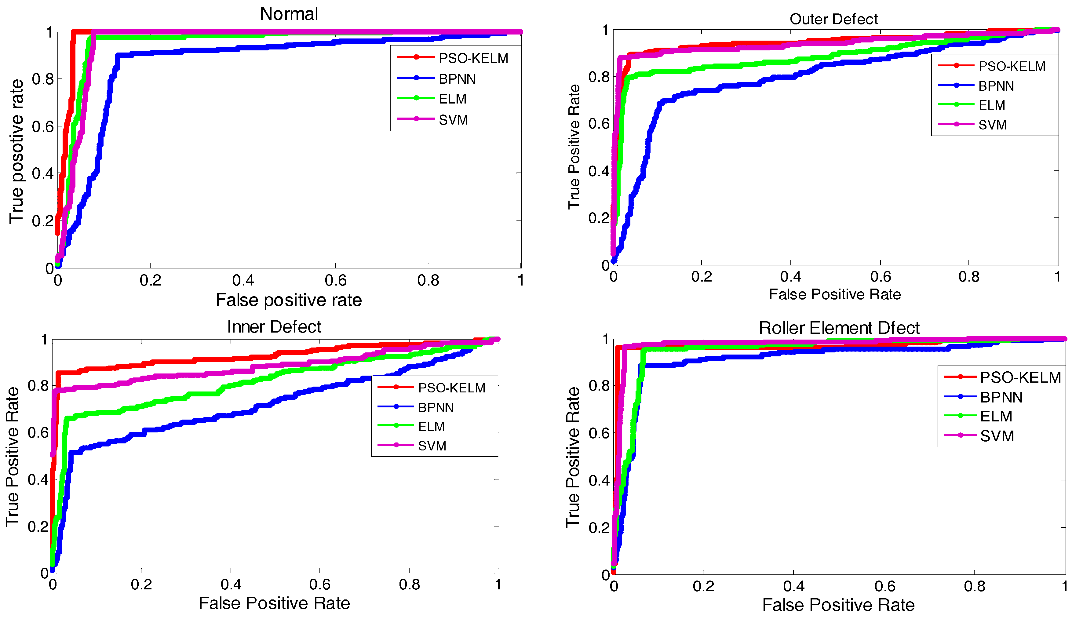
In this study, a receiver operating characteristic (ROC) curve and area under the ROC curve (AUC) are also employed to evaluate the performance of the different classifiers. Figure 15 shows the ROC curve of each classifier for condition diagnosis, and the corresponding AUC values are listed in Table 6. As shown in Figure 15 and Table 6, the AUC values of PSO-KELM are higher than that of the BP neural network, ELM, and SVM algorithms, which shows that PSO-KELM has the best classification performance.
To further verify the diagnostic capability of the method proposed in this paper in various operating conditions, the bearing vibration signal in two kinds of failure dimensions are measured for condition diagnosis, and the measuring speed is set to 600 rpm, 800 rpm, 1000 rpm, and 1200 rpm, respectively. The diagnostic results are listed in Table 7. From Table 7, with the increase in rotating speed and fault dimension, the diagnostic accuracy of the PSO-KELM algorithm is improved. The overall accuracy of PSO-KELM in various operating conditions is greater than 80%, and the highest accuracy can reach 95.02%.
The above diagnosis results demonstrate the effectiveness of the fault diagnosis method proposed in this paper for rolling bearing state monitoring and identification.
6. Conclusions
In this paper, a VMD and improved KELM-based rolling bearing state identification method is proposed. To address inconspicuous fault feature signals of rolling bearings in early fault stages and the challenge of feature extraction, the VMD method and ApEn are combined to extract fault features, and a mode number fluctuation method is proposed to determine the mode decomposition number for signal feature extraction. A simulation test shows that this method is superior to conventional EMD and LMD in terms of mode anti-aliasing and anti-noise performance. When fault diagnosis is based on the KELM method, the penalty coefficient C and kernel function parameter σ have significant impacts on the KELM performance; employing optimal parameters is the key to improving the KELM method’s state forecast accuracy. Therefore, a PSO optimization-based KELM bearing state identification method is proposed in this paper; this method optimizes the KELM parameters using a PSO optimization algorithm to obtain a KELM forecast model with optimal parameters. An analysis of rotor test bed data reveals that the proposed rolling bearing fault diagnosis method based on combination of VMD, ApEn, and PSO-KELM is effective for bearing state mode identification in various states. Compared with the BP neural network and conventional ELM and SVM algorithms, the fault diagnosis method proposed in this paper has higher diagnosis accuracy and can achieve a more accurate identification of bearing fault states. In addition, state identification of the bearing in various operating conditions is also performed by using the methods proposed in this paper. The diagnostic results show that the diagnostic accuracy of the PSO-KELM algorithm is improved with an increase in rotating speed and fault dimension, the overall accuracy of PSO-KELM is greater than 80%, and the highest accuracy can reach 95.02%. The results further demonstrate the effectiveness of the methods proposed in this paper.
Acknowledgments
The authors would like to acknowledge the National Natural Science Foundation of China (51775243, 51675035), Key Project of Industry Foresight and Common Key Technologies of Science and Technology Department of Jiangsu Province (BE2017002-2), and Fundamental Research Funds for the Central Universities (Grant No. JUSRP51732B).
Author Contributions
Ke Li and Peng Chen conceived and designed the experiments; Ke Li, Huaqing Wang and Jingjing Wu performed the experiments; Ke Li, Huaqing Wang, and Su Lei analyzed the data; Ke Li wrote the paper.
Conflicts of Interest
The authors declare no conflict of interest.
References
- Pacas, M.; Villwock, S.; Dietrich, R. Bearing damage detection in permanent magnet synchronous machines. Proc. IEEE ECCE 2009, 9, 1098–1103. [Google Scholar] [CrossRef]
- Liu, Y.; He, B.; Liu, F.; Lu, S.; Zhao, Y. Feature fusion using kernel joint approximate diagonalization of eigen-matrices for rolling bearing fault identification. J. Sound Vib. 2016, 385, 389–401. [Google Scholar] [CrossRef]
- Huang, N.E.; Shen, Z.; Long, S.R.; Wu, M.C.; Shih, H.H.; Zheng, Q.; Yen, N.; Tung, C.C.; Liu, H.H.; Smith, J.S. The empirical mode decomposition and the Hilbert spectrum for nonlinear and non-stationary time series analysis. Proc. R. Soc. Lond. Ser. A-Math. Phys. Eng. Sci. 1998, 454, 903–905. [Google Scholar] [CrossRef]
- Wang, L.Y.; Wang, Q.; Zhang, M.J.; Li, H.-L.; Zhao, W. A grey fault diagnosis method for rolling bearings based on EMD. J. Vib. Shock 2014, 33, 197–202. (In Chinese) [Google Scholar]
- Cheng, J.S.; De, D.J.; Yang, Y. A Fault Diagnosis Approach for Roller Bearing Based on SVM and EMD Envelope Spectrum. Syst. Eng. Theory Pract. 2005, 25, 131–136. [Google Scholar]
- Ali, J.B.; Fnaiech, N.; Saidi, L.; Chebel-Morello, B.; Fnaiecha, F. Application of empirical mode decomposition and artificial neural network for automatic bearing fault diagnosis based on vibration signals. Appl. Acoust. 2015, 89, 16–27. [Google Scholar] [CrossRef]
- Smith, J.S. The local mean decomposition and its application to EEG perception data. J. R. Soc. Interface 2005, 2, 443–454. [Google Scholar] [CrossRef] [PubMed]
- Chen, B.J.; He, Z.J.; Chen, X.F.; Cao, H.; Cai, G.; Zi, Y. A demodulating approach based on local mean decomposition and its applications in mechanical fault diagnosis. Meas. Sci. Technol. 2011, 22, 55704–55716. [Google Scholar] [CrossRef]
- Liu, W.Y.; Zhang, W.H.; Han, J.G.; Wang, G.F. A new wind turbine fault diagnosis method based on the local mean decomposition. Renew. Energy 2012, 48, 411–415. [Google Scholar] [CrossRef]
- Hu, A.J.; An, L.S.; Tang, G.J. New process method for effects of HILBERT-HUANG transform. Chin. J. Mech. Eng. 2008, 44, 154–158. (In Chinese) [Google Scholar] [CrossRef]
- Dragomiretskiy, K.; Zosso, D. Variational Mode Decomposition. IEEE Trans. Signal Proc. 2014, 62, 531–544. [Google Scholar] [CrossRef]
- Aneesh, C.; Kumar, S.; Hisham, P.M.; Soman, K.P. Performance Comparison of Variational Mode Decomposition over Empirical Wavelet Transform for the Classification of Power Quality Disturbances Using Support Vector Machine. Procedia Comput. Sci. 2015, 46, 372–380. [Google Scholar] [CrossRef]
- Mohanty, S.; Gupta, K.K.; Raju, K.S. Bearing fault analysis using variational mode decomposition. In Proceedings of the 9th International Conference on Industrial and Information Systems (ICIIS), Gwalior, India, 15–17 December 2014; pp. 1–6. [Google Scholar]
- Lv, Z.L.; Tang, B.P.; Zhou, Y.; Zhou, C.D. A Novel Method for Mechanical Fault Diagnosis Based on Variational Mode Decomposition and Multikernel Support Vector Machine. Shock Vib. 2016, 2016, 1–11. [Google Scholar] [CrossRef]
- Huang, G.B.; Wang, D.H.; Lan, Y. Extreme learning machines: A survey. Int. J. Mach. Learning Cybern. 2011, 2, 107–122. [Google Scholar] [CrossRef]
- He, Y.J.; Qi, M.X.; Luo, H.M. AE based fault diagnosis of rolling bearings by use of ICA and SVM. J. Vib. Shock 2008, 27, 150–153. [Google Scholar]
- An, X.; Zhao, M.; Jiang, D.; Li, S. Direct-drive wind turbine fault diagnosis based on support vector machine and multi-source information. Power Syst. Technol. 2011, 35, 117–122. (In Chinese) [Google Scholar]
- Li, P.; Li, X.J.; Jiang, L.L.; Yang, D.L. Fault Diagnosis for Motor Rotor Based on KPCA-SVM. Appl. Mech. Mater. 2012, 143–144, 680–684. [Google Scholar] [CrossRef]
- Verma, N.K.; Roy, A.; Salour, A. An optimized fault diagnosis method for reciprocating air compressors based on SVM. In Proceedings of the 2011 IEEE International Conference on System Engineering and Technology (ICSET), Shah Alam, Malaysia, 27–28 June 2011; pp. 65–69. [Google Scholar]
- Huang, G.B. An insight into extreme learning machines: Random neurons, random features and kernels. Cogn. Comput. 2014, 6, 376–390. [Google Scholar] [CrossRef]
- Wang, X.Y.; Han, M. Multivariate chaotic time series prediction using multiple kernel extreme learning machine. Acta Phys. Sin. 2015, 64, 070504. [Google Scholar] [CrossRef]
- Zhang, Y.T.; Ma, C.; Li, Z.N.; Fan, H.B. Online modeling of kernel extreme learning machine based on fast leave-one-out cross-validation. J. Shanghai Jiaotong Univ. (Sci.) 2014, 48, 641–646. [Google Scholar]
- He, Y.; Huang, J.; Zhang, B. Approximate entropy as a nonlinear feature parameter for fault diagnosis in rotating machinery. Meas. Sci. Technol. 2012, 23, 45603–45616. [Google Scholar] [CrossRef]
- Cheng, S.; Yan, J.W.; Zhao, D.F. Short Term Load Forecasting Method Based on Ensemble Improved Extreme Learning Machine. J. Xian Jiaotong. Univ. 2009, 43, 106–110. (In Chinese) [Google Scholar]
- Kennedy, R.; Eberhart, J. Particle swarm optimization. In Proceedings of the IEEE International Conference on Neural Networks, Perth, Australia, 27 November–1 December 1995; Volume 4, pp. 1942–1948. [Google Scholar]
- Li, K.; Ping, X.; Wang, H.; Chen, P.; Cao, Y. Sequential Fuzzy Diagnosis Method for Motor Roller Bearing in Variable Operating Conditions Based on Vibration Analysis. Sensors 2013, 13, 8013–8041. [Google Scholar] [CrossRef] [PubMed]
- Debnath, R.; Takahide, N.; Takahashi, H. A decision based one-against-one method for multi-class support vector machine. Pattern Anal. Appl. 2004, 7, 164–175. [Google Scholar] [CrossRef]
Figure 1.
Method for determining the number of variational mode decomposition (VMD) modes.

Figure 2.
Simulation signals: (a) composite signal y(t); (b) interval signal x1(t); (c) linear frequency modulation signal x2(t), and (d) cosine signal x3(t).
Figure 2.
Simulation signals: (a) composite signal y(t); (b) interval signal x1(t); (c) linear frequency modulation signal x2(t), and (d) cosine signal x3(t).
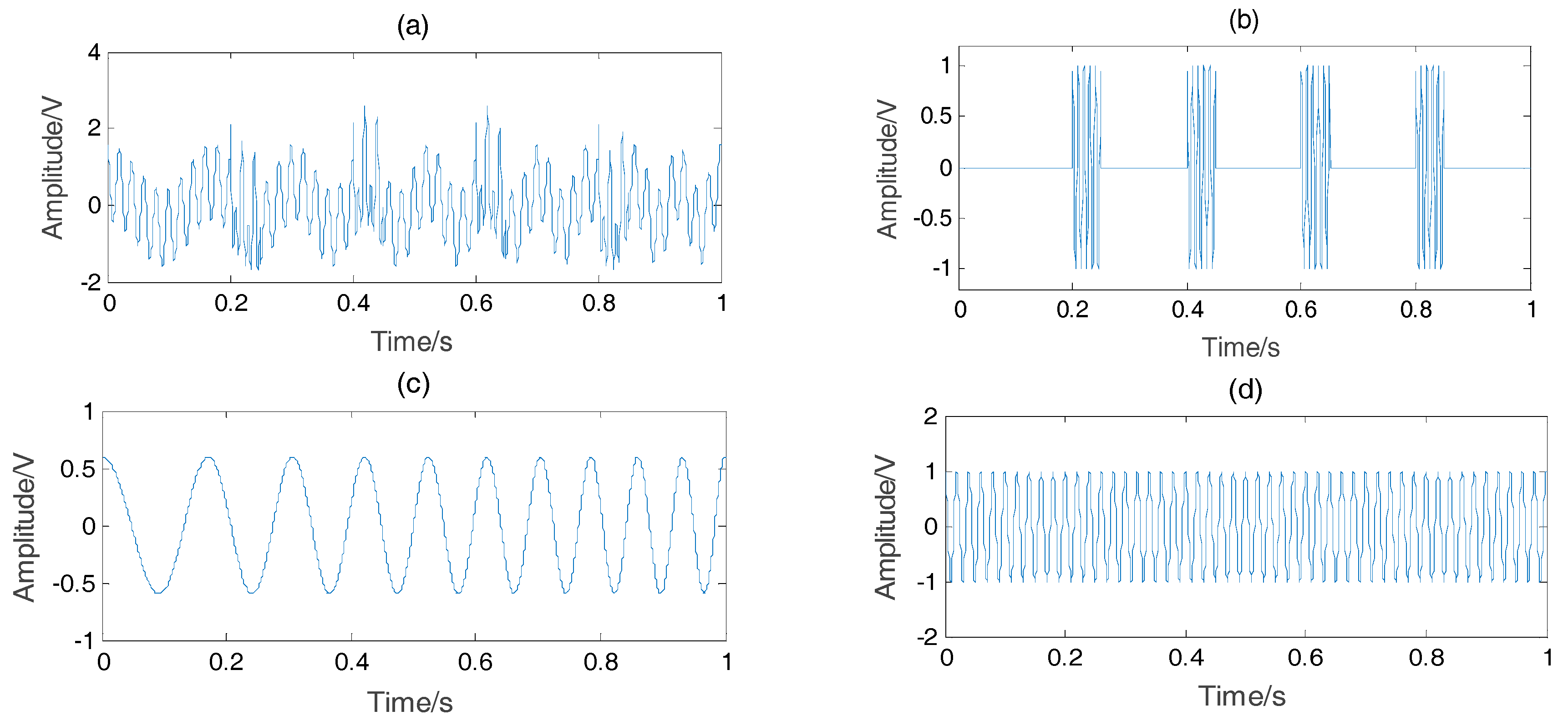
Figure 3.
Simulation signal y(t) VMD results. (a) IMF1; (b) IMF2; (c) IMF3.
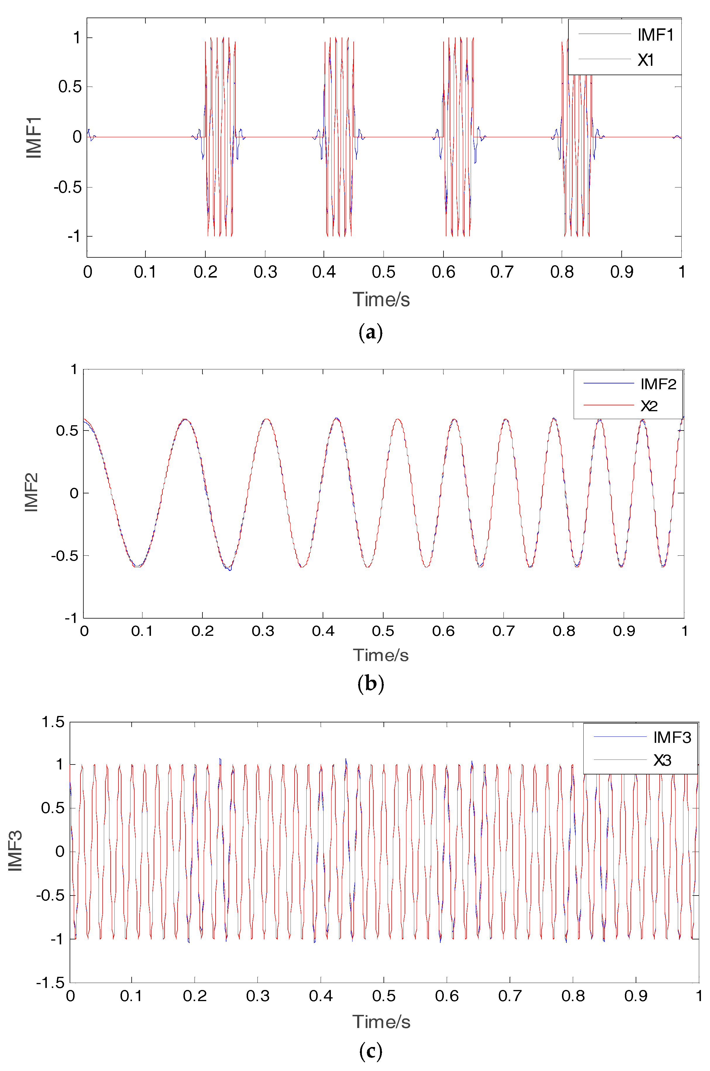
Figure 4.
Simulation signal y(t) empirical mode decomposition (EMD) results.

Figure 5.
Simulation signal y(t) local mean decomposition (LMD) result. PF (Product function).
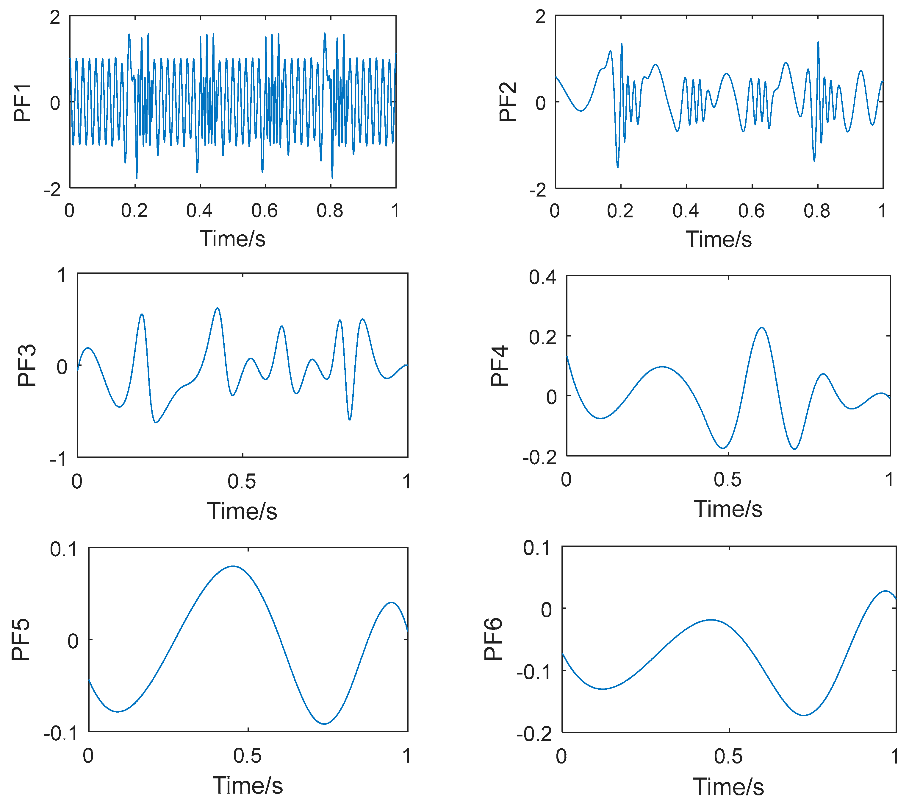
Figure 6.
Centrifugal fan for condition diagnosis: (a) illustration of a centrifugal fan; and (b) photograph of a centrifugal fan.
Figure 6.
Centrifugal fan for condition diagnosis: (a) illustration of a centrifugal fan; and (b) photograph of a centrifugal fan.
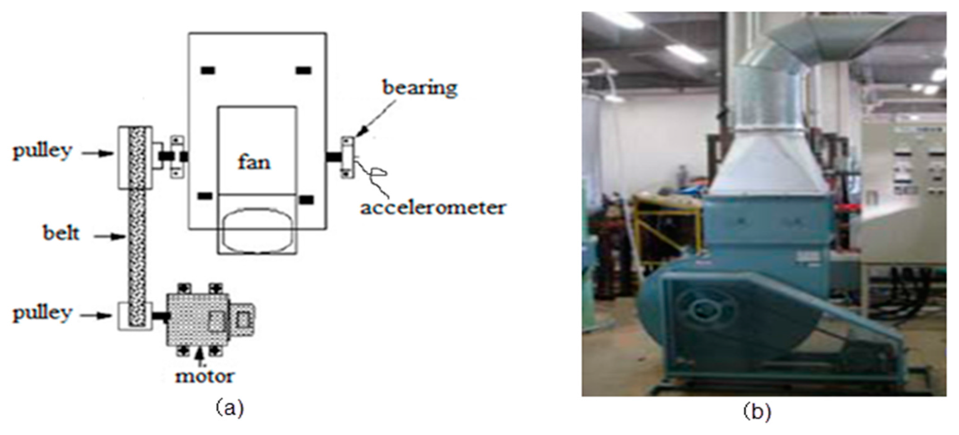
Figure 7.
Bearing for condition diagnosis: (a) inner ring defect; (b) outer ring defect; and (c) roller element defect.
Figure 7.
Bearing for condition diagnosis: (a) inner ring defect; (b) outer ring defect; and (c) roller element defect.
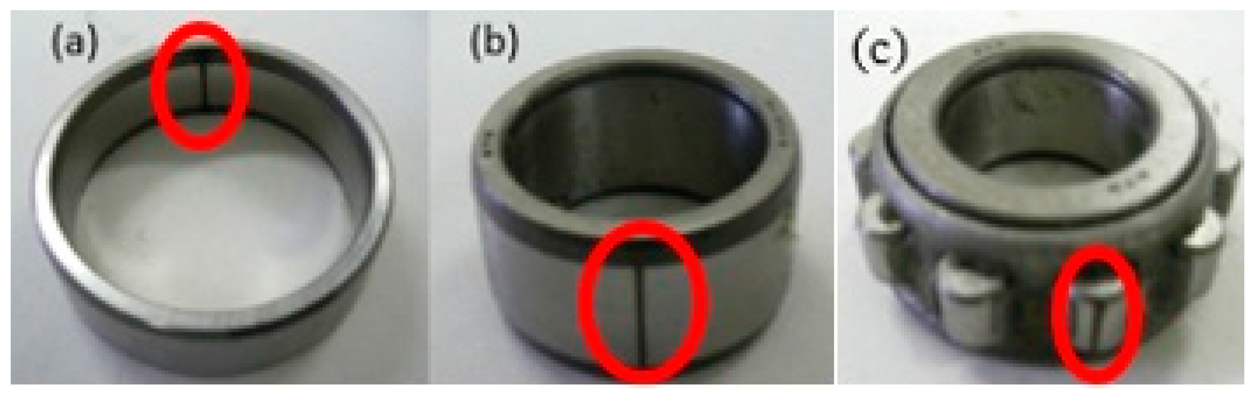
Figure 8.
Vibration signal in each state: (a) normal; (b) outer ring defect; (c) inner ring defect; and (d) rolling element defect.
Figure 8.
Vibration signal in each state: (a) normal; (b) outer ring defect; (c) inner ring defect; and (d) rolling element defect.

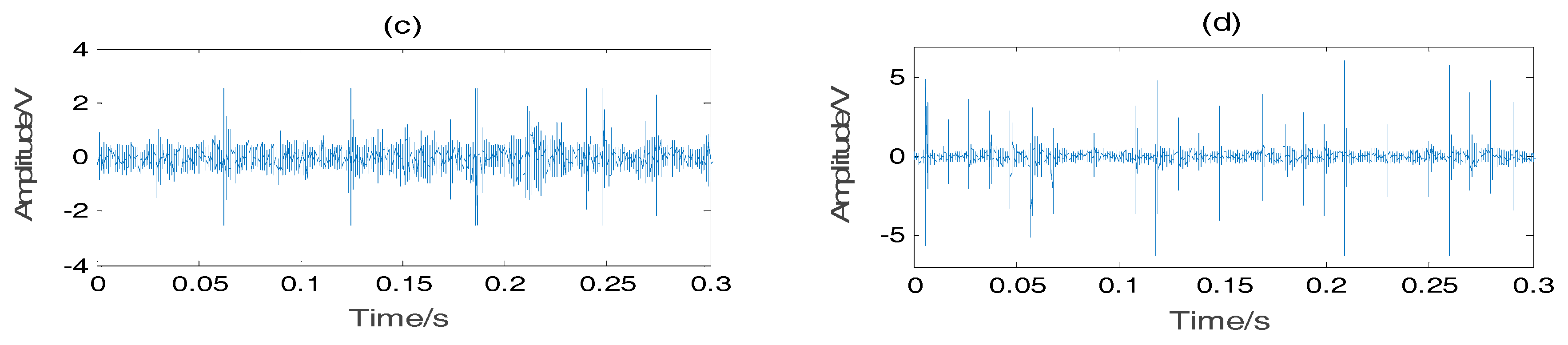
Figure 9.
Fault diagnosis process. ApEn: approximate entropy; PSO: particle swarm optimization; CV: cross validation; KELM: kernel extreme learning machine.
Figure 9.
Fault diagnosis process. ApEn: approximate entropy; PSO: particle swarm optimization; CV: cross validation; KELM: kernel extreme learning machine.

Figure 10.
Normal state signal VMD.
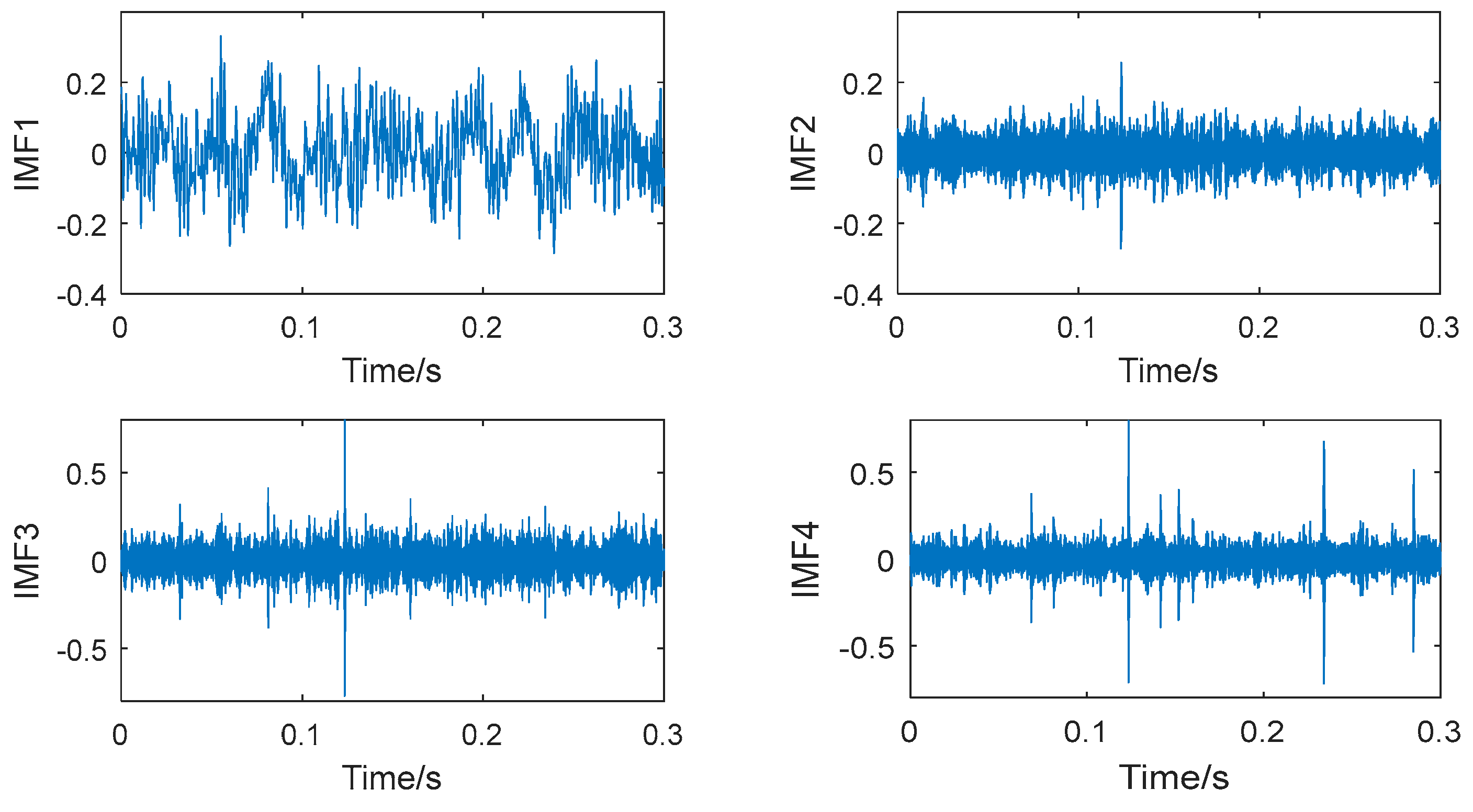
Figure 11.
Outer ring defect state signal VMD.

Figure 12.
Inner ring defect state signal VMD.
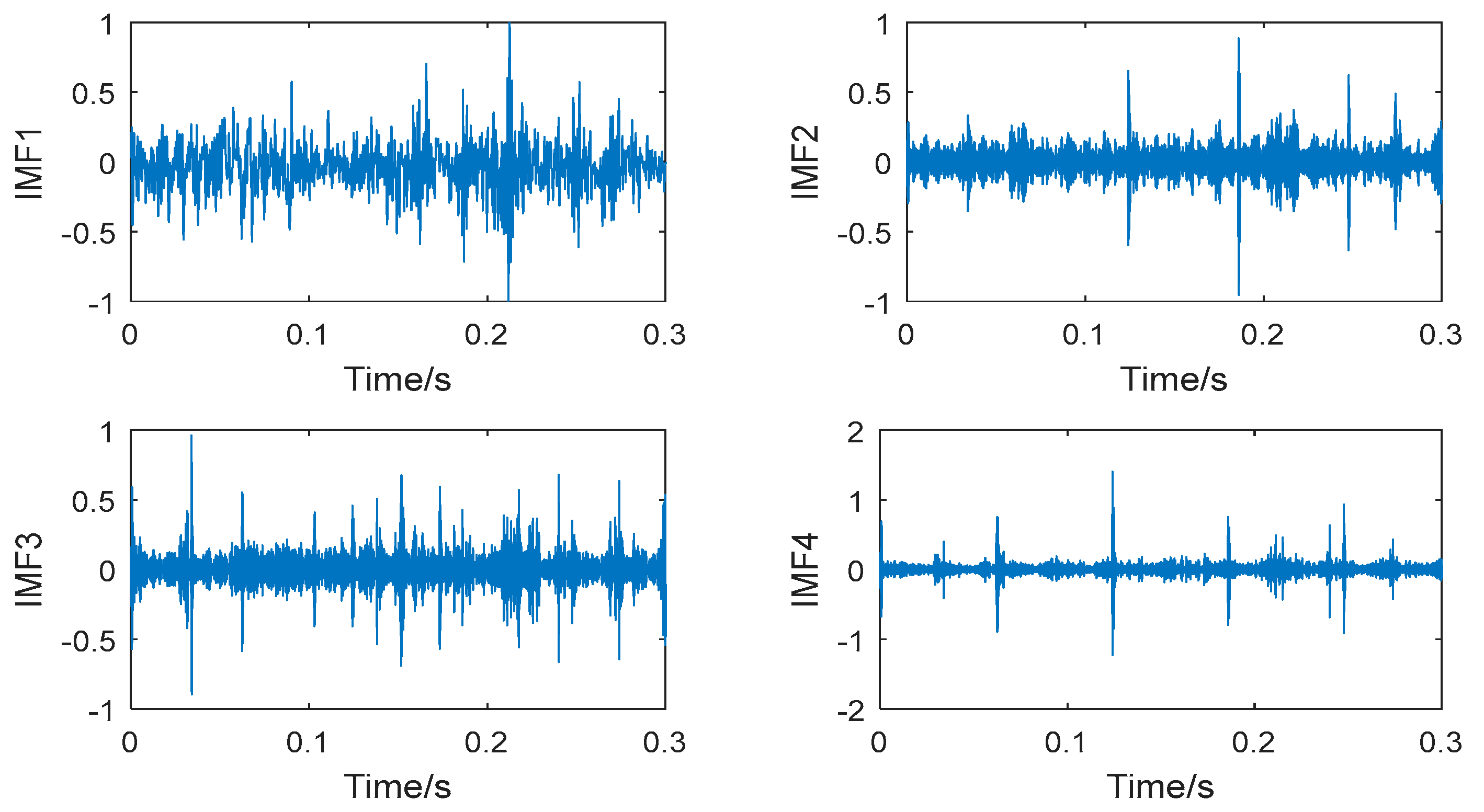
Figure 13.
Roller defect state signal VMD.
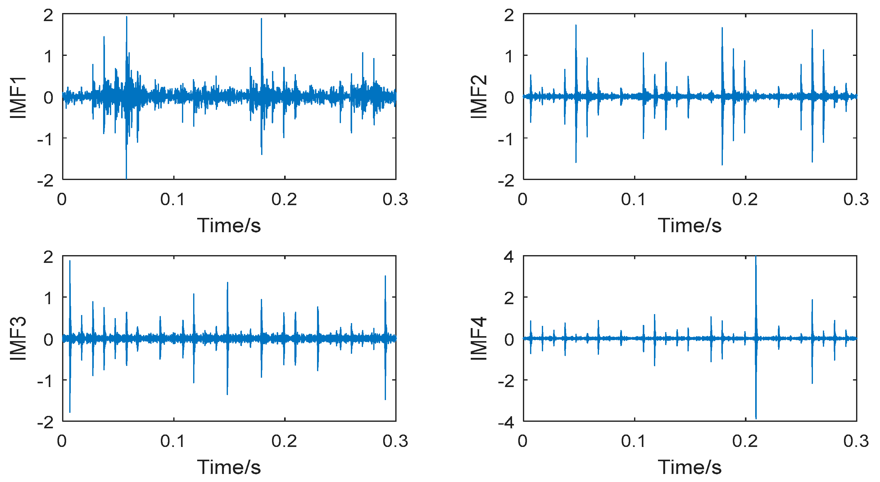
Figure 14.
PSO-KELM (particle swarm optimization-kernel extreme learning machine) algorithm procedure.
Figure 14.
PSO-KELM (particle swarm optimization-kernel extreme learning machine) algorithm procedure.
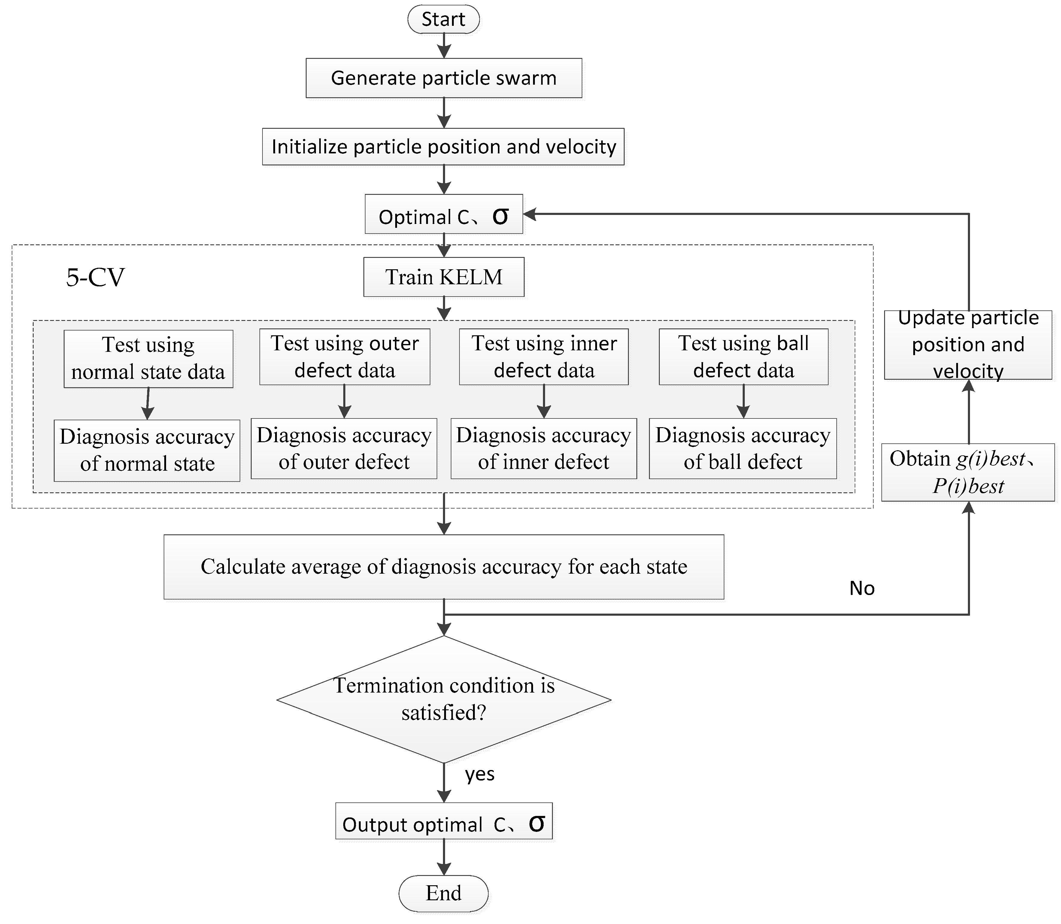
Figure 15.
Receiver operating characteristic (ROC) curve of each classifier.


Table 1.
Bearing parameters for verification.
| Contents | Parameters |
|---|---|
| Bearing outer diameter | 52 mm |
| Bearing inner diameter | 25 mm |
| Bearing width | 15 mm |
| Bearing roller diameter | 7 mm |
| The number of the rollers | 11 |
| Contact angle | 0 rad |
| Outer defect | 0.3 × 0.05 mm (width × depth) |
| Inner defect | 0.3 × 0.05 mm (width × depth) |
| Roller element defect | 0.3 × 0.05 mm (width × depth) |
Table 2.
Detection index (DI) values of each symptom parameter (SP).
| DI Values | Symptom Parameters | ||||||
|---|---|---|---|---|---|---|---|
| RMS (Root Mean Square) | Skewness | Kurtosis | ApEn1 | ApEn2 | ApEn3 | ApEn4 | |
| DIN-O | 1.26 | 1.536 | 1.284 | 1.662 | 2.119 | 5.376 | 6.931 |
| DIN-I | 0.828 | 1.344 | 2.868 | 1.332 | 8.675 | 2.098 | 9.341 |
| DIN-R | 1.232 | 0.864 | 1.356 | 11.813 | 8.103 | 6.769 | 6.280 |
| DIO-I | 2.108 | 1.176 | 2.412 | 0.918 | 5.572 | 8.268 | 2.779 |
| DIO-R | 1.136 | 0.696 | 1.656 | 3.079 | 24.526 | 3.918 | 2.468 |
| DII-R | 2.352 | 0.348 | 1.92 | 1.256 | 17.051 | 8.059 | 0.527 |
Here, N, O, I, R indicate normal, outer ring defect, inner ring defect and roller element defect states, respectively. RMS: root mean square.
Table 3.
Distribution information of the ApEn.
| Apen | Normal State | Outer Ring Defect | Inner Ring Defect | Roller Element Defect | ||||
|---|---|---|---|---|---|---|---|---|
| Average | Standard Deviation | Average | Standard Deviation | Average | Standard Deviation | Average | Standard Deviation | |
| ApEn1 | 0.731 | 0.010 | 0.145 | 0.021 | 0.405 | 0.083 | 0.434 | 0.012 |
| ApEn2 | 0.712 | 0.012 | 0.221 | 0.030 | 0.841 | 0.013 | 0.790 | 0.051 |
| ApEn3 | 0.691 | 0.031 | 0.458 | 0.031 | 0.578 | 0.029 | 1.005 | 0.061 |
| ApEn4 | 0.670 | 0.005 | 0.997 | 0.012 | 1.044 | 0.050 | 1.066 | 0.104 |
Table 4.
Training data for each state.
| Approximate Entropy | State | ||||||
|---|---|---|---|---|---|---|---|
| IMF1 | IMF2 | IMF3 | IMF4 | Normal | Outer Defect | Inner Defect | Element Defect |
| 0.72001 | 0.14866 | 0.40609 | 0.42288 | 1 | 0 | 0 | 0 |
| 0.72055 | 0.14759 | 0.40633 | 0.42241 | 1 | 0 | 0 | 0 |
| 0.72071 | 0.14726 | 0.40579 | 0.42055 | 1 | 0 | 0 | 0 |
| 0.71503 | 0.224 | 0.84966 | 0.78457 | 0 | 1 | 0 | 0 |
| 0.71519 | 0.22413 | 0.84976 | 0.78629 | 0 | 1 | 0 | 0 |
| 0.69023 | 0.45486 | 0.60378 | 0.99773 | 0 | 1 | 0 | 0 |
| 0.68705 | 0.46803 | 0.5576 | 1.0275 | 0 | 0 | 1 | 0 |
| 0.68699 | 0.46578 | 0.55627 | 1.0291 | 0 | 0 | 1 | 0 |
| 0.69023 | 0.45486 | 0.60378 | 0.99773 | 0 | 0 | 1 | 0 |
| 0.68039 | 0.99442 | 1.0432 | 1.0662 | 0 | 0 | 0 | 1 |
| 0.68052 | 0.995 | 1.043 | 1.0649 | 0 | 0 | 0 | 1 |
| 0.68109 | 0.9989 | 1.0441 | 1.0666 | 0 | 0 | 0 | 1 |
Table 5.
Comparison results of different algorithm.
| Classifier | Average Diagnostic Accuracy % | Overall Accuracy % | |||
|---|---|---|---|---|---|
| N | O | I | R | ||
| BPNN | 90.0 | 68.7 | 51.7 | 88.6 | 74.75 |
| ELM | 97.3 | 79.0 | 66 | 95.6 | 84.48 |
| SVM | 100 | 88.7 | 77.4 | 96.8 | 90.73 |
| PSO-KELM | 100 | 90.3 | 85.7 | 96.3 | 93.08 |
BPNN: Back Propagation Neural Network; ELM: extreme learning machine; SVM: support vector machine; PSO-KELM: particle swarm optimization-kernel extreme learning machine.
Table 6.
Area under the ROC curve (AUC) values of each classifier.
| Classifier | Bearing State | |||
|---|---|---|---|---|
| Normal | Outer Defect | Inner Defect | Roller Element Defect | |
| BPNN | 0.871 | 0.805 | 0.720 | 0.911 |
| ELM | 0.953 | 0.883 | 0.815 | 0.948 |
| SVM | 0.956 | 0.935 | 0.883 | 0.974 |
| PSO-KELM | 0.981 | 0.939 | 0.925 | 0.965 |
Table 7.
Diagnostic results in different operating conditions.
| Fault Dimension (Width × Depth) mm | Speed rpm | Diagnostic Accuracy (%) | Overall Accuracy (%) | |||
|---|---|---|---|---|---|---|
| N | O | I | R | |||
| 0.3 × 0.05 | 600 | 98.2 | 84.6 | 78.4 | 62.3 | 80.87 |
| 800 | 100 | 86.3 | 78.9 | 86.2 | 87.85 | |
| 1000 | 100 | 90.3 | 85.7 | 96.3 | 93.08 | |
| 1200 | 100 | 93.7 | 84.6 | 96.8 | 93.77 | |
| 0.3 × 0.15 | 600 | 100 | 88.7 | 84.2 | 75.3 | 87.05 |
| 800 | 100 | 91.5 | 84.6 | 90.6 | 91.67 | |
| 1000 | 100 | 93.2 | 87.9 | 96.9 | 94.5 | |
| 1200 | 100 | 93.8 | 88.1 | 98.2 | 95.02 | |
© 2017 by the authors. Licensee MDPI, Basel, Switzerland. This article is an open access article distributed under the terms and conditions of the Creative Commons Attribution (CC BY) license (http://creativecommons.org/licenses/by/4.0/).
Share and Cite
MDPI and ACS Style
Li, K.; Su, L.; Wu, J.; Wang, H.; Chen, P. A Rolling Bearing Fault Diagnosis Method Based on Variational Mode Decomposition and an Improved Kernel Extreme Learning Machine. Appl. Sci. 2017, 7, 1004. https://doi.org/10.3390/app7101004
AMA Style
Li K, Su L, Wu J, Wang H, Chen P. A Rolling Bearing Fault Diagnosis Method Based on Variational Mode Decomposition and an Improved Kernel Extreme Learning Machine. Applied Sciences. 2017; 7(10):1004. https://doi.org/10.3390/app7101004
Chicago/Turabian StyleLi, Ke, Lei Su, Jingjing Wu, Huaqing Wang, and Peng Chen. 2017. "A Rolling Bearing Fault Diagnosis Method Based on Variational Mode Decomposition and an Improved Kernel Extreme Learning Machine" Applied Sciences 7, no. 10: 1004. https://doi.org/10.3390/app7101004
Note that from the first issue of 2016, this journal uses article numbers instead of page numbers. See further details here.