A Comparative Study of Clustering Analysis Method for Driver’s Steering Intention Classification and Identification under Different Typical Conditions

Abstract

Driver’s intention classification and identification is identified as the key technology for intelligent vehicles and is widely used in a variety of advanced driver assistant systems (ADAS). To study driver’s steering intention under different typical operating conditions, five driving school coaches of different ages and genders are selected as the test drivers for a real vehicle test. Four kinds of typical car steering condition test data with four different vehicles are collected. Test data are filtered by the Butterworth filter and are used for extracting the driver steering characteristic parameters. Based on Principal Component Analysis (PCA), the three kinds of clustering analysis methods, including the Fuzzy C-Means algorithm (FCM), the Gustafson–Kessel algorithm (GK) and the Gath–Geva algorithm (GG), considered are proposed to classify and identify driver’s intention under different typical operating conditions. Results show that the three approaches can successfully classify and identify drivers’ intention respectively despite some accuracy error by FCM. Meanwhile, compared with FCM and GK, GG was the best performing in classification and identification of the driver’s intention. In order to verify the validity of the identification method designed by this article, five different drivers were selected. Five tests were carried out on the driving simulator. The results show that the results of each identification are exactly the same as the actual driver’s intention.

1. Introduction

In recent years, with the rapid integration of high-tech and advanced automotive technologies such as computers, the Internet, communications and navigation, automatic control, artificial intelligence, machine vision, precision sensors, high-precision maps and smart cars (or unmanned vehicles), smart driving has become one of the world’s automotive engineering research hotspots and a new impetus of the automotive industry’s growth. According to authoritative media at home and abroad, in the future of the automotive industry, more than 90% of scientific and technological innovation will focus on the field of automotive intelligence. Therefore, smart vehicles are safe, efficient, energy-efficient next-generation vehicles [1,2], and the study of smart cars has a very important significance, which has become the focus of the global automotive industry.

The driver intention is reflected by his/her own inner state in the driving process. It cannot be obtained directly during driving and is only predicted by the driver’s movements, vehicle status and traffic environment information. Driver’s intention classification and identification are identified as comprising the key technology for intelligent vehicles and are widely used in a variety of Advanced Driver Assistant Systems (ADAS) [3,4], such as the Adaptive Cruise Control System (ACC) [5,6], the Active Front Steering System (AFS) [7,8,9,10], the Parking Assistance Systems (PAS) [11,12], the steer-by-wire systems [13] and Man-machine Co-driving Electric Power Steering (MCEPS) system [14,15]. The classification and identification of driver’s intention are based on the real-time acquisition of the driver’s operating signal and car state, or at the same time, by monitoring the driver’s head movement range and facial expressions, the driver’s behavior is distinguished and identified to obtain the driver’s driving intention [16].

Many scholars are committed to study the classification and identification of driver’s intention. Liang Li et al. [17] proposed a novel method based on an artificial error back-propagation neural network to identify the driver’s starting intention. Takano et al. [18] proposed an intelligent cognitive method for driver’s intention identification based on the Hidden Markov Model (HMM). The method mainly includes data segmentation, time series data labeling and the identification and generation of the driving mode. Raksin et al. [19] proposed an algorithm based on the driver’s intention to identify the direct yaw moment control, in which the driver steering intention identification is through the Hidden Markov Model (HMM). The use of the dynamic Bayesian network was combined with the past driving state and the current driving state to predict the driver’s intention of parking at the crossroads. Tesheng Hsiao [20] used the maximum posterior probability assessment method to obtain the driver’s steering model parameters. He established a steering model that can effectively improve the recognition accuracy and that has the function of predicting the driver’s driving strategy. The previous research works mainly concentrated on a single traffic environment, such as the straight road or the crossroads intentions, and not on variety of typical steering conditions under the driving intention identification study.

The driving intention under each condition requires multiple drivers’ characteristic steering parameters, such as driving parameters (steering angle, angular velocity and torque) and vehicle status parameters (roll angle, lateral acceleration and yaw rate). However, if all the characteristic parameters are used for classification and identification, the computational complexity is increased due to the large number of characteristic parameters. Additionally, analysis of the situation becomes much more difficult. Although each feature parameter provides some information, some of the characteristic parameters are correlated, and the characteristic parameters are not independent of each other. Therefore, the information provided by these characteristic parameters overlaps to some extent. Therefore, we need to use a kind of theoretical algorithm to reduce the dimension of the data and to decorrelate the input variables. Principal Component Analysis (PCA) is used to reduce the data dimension, which is used in various applications such as error recognition [21], pedestrian identification [22] and image tracking [23]. However, PCA is not used in the driving intention identification study under typical steering conditions.

In essence, the driver’s intention is a pattern recognition process. The cluster analysis is a typical method of pattern recognition. Compared with the traditional classification and identification of driver’s intention using the neural network and fuzzy mathematics, the clustering algorithm only needs a small amount of data, which eliminates the need to construct the nonlinear recognizer and ensures that the accuracy is stable. In order to classify and identify driver’s intention, three clustering analysis methods are studied: the Fuzzy C-Means algorithm (FCM), the Gustafson–Kessel algorithm (GK) and the Gath–Geva algorithm (GG). Due to its flexibility and robustness for ambiguity, the FCM algorithm is currently an active topic [24] and has been widely applied in the areas of pattern recognition [25], function approximation [26], image processing [27], machine learning [28], and so on. The GK algorithm can generate a fuzzy partition that provides the degree of membership of each data point to a given cluster [29]. The GG algorithm can make the parameters of the univariate membership functions be directly derived from the parameters of the clusters [30].

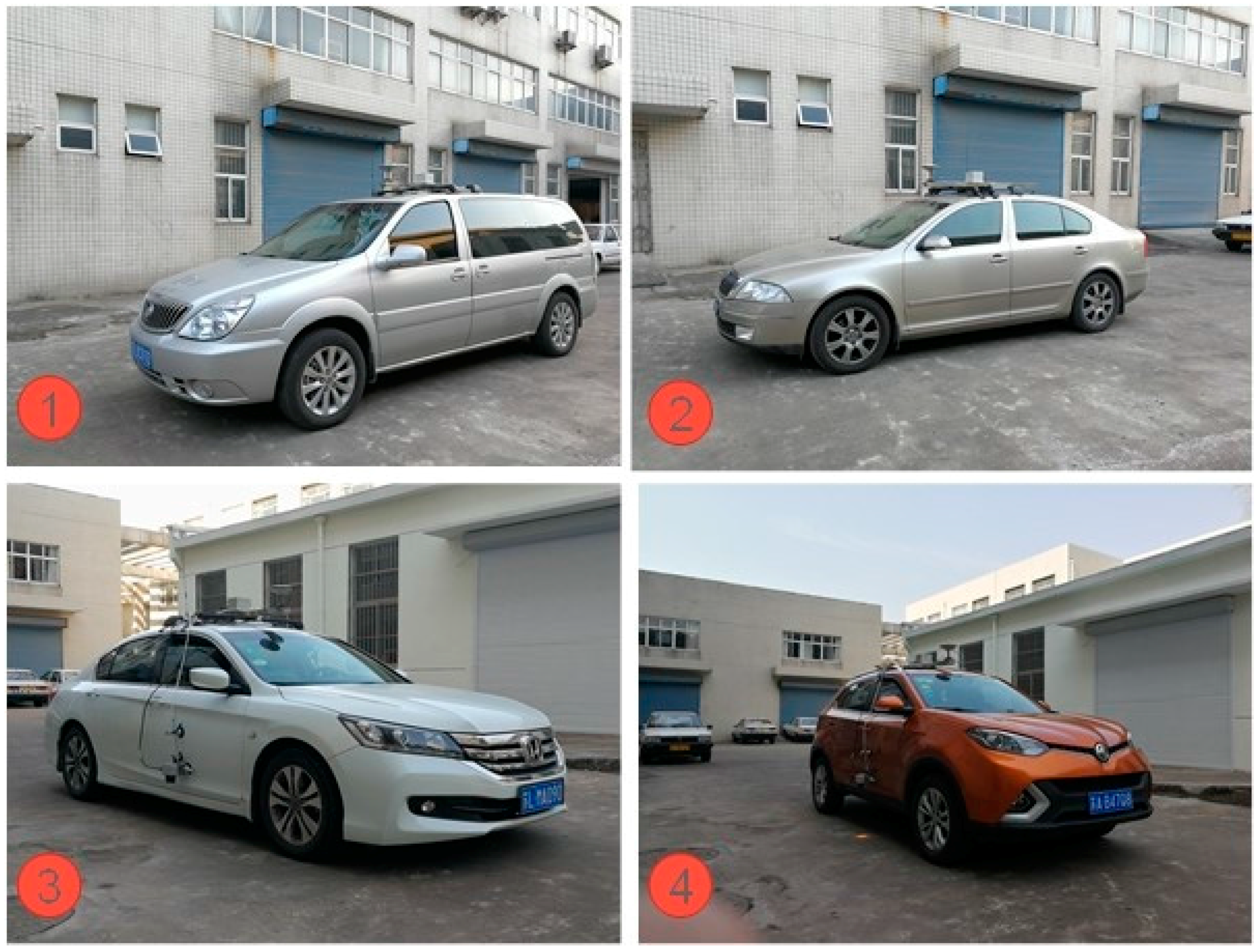
Therefore, this paper selected five driving school coaches of different driving experiences and genders as real vehicle test driver, and four typical car steering conditions’ test data with four different vehicles were collected. Additionally, this paper used principal component analysis and clustering analysis to classify and identify the driver’s intention. The paper analyzed the advantages and disadvantages of the three different clustering methods (FCM, GK and GG) in the direction of driver’s steering intention.

The paper is organized as follows. In the second section, five driving school coaches of different ages and genders are selected as the test drivers for the real vehicle test. In the third section, driver’s characteristic steering parameters under different conditions are proposed. The fourth section uses principal component analysis and clustering analysis to classify and identify the driver’s intention. In the fifth section, the clustering results and analysis are presented. Finally, the conclusions are drawn in the last section.

2. Experiment

2.1. Experimental Devices

The real vehicle experiment of driver’s steering in different conditions consists of the following components: S-Motion biaxial optical speed sensor (Kistler, Winterthur, Switzerland) (signal delay only 6 ms), biaxial optical speed sensor mounting bracket, KiMSW Force steering wheel sensor 250 Nm (Kistler, Winterthur, Switzerland) (steering angle accuracy: 0.015°), universal mounting bracket (Kistler, Winterthur, Switzerland), power distribution box (Kistler, Winterthur, Switzerland) and SDI-600GI Model GPS/INS (SDI, Beijing, China) (accuracy: 10 cm error). The experimental devices are shown in Figure 1.

2.2. Experimental Design and Experimental Vehicles

This experiment selected 5 driving school coaches of different driving ages and genders as the test drivers, which are shown in

Table 1. Driver information.

No.	Ages (Years)	Driving Experience (Years)	Gender
Driver 1	55	33	female
Driver 2	28	10	male
Driver 3	53	31	male
Driver 4	46	22	male
Driver 5	53	21	male

. The turn right/left steering condition, U-turn condition, lane keeping condition and lane changing condition are proposed in the real vehicle test. Additionally, the speed of the vehicle is certain during the test. The test vehicles were four passenger cars: GM GL8, Skoda Octavia, Honda Accord and SAIC MG. The experimental vehicles are shown in Figure 2.

3. The Method of the Driver’s Intention Identification

Driver’s Characteristic Steering Parameter under Different Conditions

In order to accurately describe the steering characteristics of the driver under each steering condition, it is ensured that there will be no loss or distortion of the driver’s intention information. According to GB/T 6323-1994 “Vehicle Handling Stability Test Method”, this paper selects the typical steering conditions of the driver’s characteristic parameters, as shown in

Table 2. Driver’s characteristic steering parameters.

Symbol	Meaning	Units
${\delta }_m$	Average steering angle	deg
${\delta }_{\max }$	Maximum steering angle	deg
${\dot{\delta }}_{\mathrm{m}}$	Average angular velocity	deg/s
${\dot{\delta }}_{\max }$	Maximum angular velocity	deg/s
$T_m$	Average torque	Nm
$T_{\max }$	Maximum torque	Nm
${\gamma }_{\max }$	Maximum yaw rate	deg/s
${\varphi }_{\max }$	Maximum roll angle	deg
$a_y{}_{{}_{\max }}$	Maximum lateral acceleration	m/s2

. In order to identify the driver’s steering intention under different steering conditions, this paper chooses the driver steering parameters and vehicle dynamics parameters for the first two seconds under different operating conditions. The purpose of this is to use the initial operation of the driver to identify the driver’s steering intention in the next period. It is helpful to lay the foundation for dynamic control for further advanced driver assistant systems. Furthermore, this can improve the accuracy of the intelligent vehicle active safety control system. However, various uncertainties exist due to the large amount of interference signal in the test data, as shown in Figure 3. Especially, torque, angular velocity, yaw rate and lateral acceleration need to be filtered.

The Butterworth filter is a kind of electronic filter whose frequency response curve is the smoothest. The filter was first proposed by a British engineer, Stephen Butterworth, in a paper published in the British journal Radio Engineering in 1930. The attenuation rate of the first-order Butterworth filter is 6 dB per octave. The second-order Butterworth filter has a decay rate of 12 dB per octave, and the third-order Butterworth filter has an attenuation rate of 18 dB per octave, and so on. The amplitude of the Butterworth filter is monotonically decreasing, and it is also the only filter that maintains the same shape regardless of the order of the amplitude of the diagonal frequency curve. The higher the order of the filter is, the faster the amplitude attenuation in the resistive band is. The difference with the Chebyshev, Bessel and elliptical filters is that the attenuation of the Butterworth filter is slower than the other filters, but is very flat and does not vary.

The Butterworth low-pass filter can be expressed by the square of the amplitude:

$${\left|H\left(\omega \right)\right|}^2=\frac{1}{1+{\left(\frac{\omega }{{\omega }_c}\right)}^{2n}}$$

(1)

where n is the order of the filter and ${\omega }_c$ is the cut-off frequency.

Therefore, we choose the Butterworth filter with different orders to process the test data. Filter results can be seen in Figure 3. In Figure 3a, the first-order Butterworth filter obtains the closest data to the raw data; simultaneously, the value of torque is also very smooth. Therefore, the first-order Butterworth filter is the most suitable to handle the torque signal. In Figure 3b, we can reach the same conclusion about the angular velocity signal. In Figure 3c,d, although the first-order Butterworth filter obtains the closest data to the raw data, the first-order Butterworth filter is less smooth than the second-order Butterworth filter. Therefore, the second-order Butterworth filter is the most suitable to handle the yaw rate and the lateral acceleration signal.

Since the number of experimental data is very large, which is shown in

Table 3. Actual experimental data and speed conditions.

The Number of Experiment and the Speed Limit	Typical Steering Conditions
	Turning Right/Left Condition	U-Turn Condition	Lane Keeping Condition	Lane Changing Condition	The Sum of All the Conditions
Number of Experimental Data	320	82	160	162	724
Speed Conditions (km/h)	20–50	20–30	30–60	30–40	20–60

, only about 20% (133) of the experimental data are selected (after removing the wrong data). This is because, compared with the traditional classification and identification of the driver’s intention using the neural network and fuzzy mathematics, the clustering algorithm only needs a small amount of data, which eliminates the need to construct the nonlinear recognizer and ensures that the accuracy is stable. Additionally, the characteristic parameters of these sets of test data are extracted and analyzed, which lays the foundation for the driver’s steering intention identification.

The representative samples of the experimental data of the real vehicle tests are shown in Figure 4, Figure 5, Figure 6, Figure 7, Figure 8 and Figure 9, which contain four conditions of the data, respectively, turning right condition, U-turn condition, lane keeping condition and lane changing condition.

4. Principal Component Analysis of Steering Parameters

In solving practical problems and research, it is often possible to collect more information about the research object in order to have a comprehensive understanding of the problem. However, due to the theoretical development and application of technical constraints, having too many variables to be processed and too much information have become analysis obstacles. To solve this problem, Principal Component Analysis (PCA) should be used to analyze data. PCA is a statistical analysis method that simplifies multiple indicators into a small number of comprehensive indicators, with as few as possible to reflect the original variable information [31], to ensure that the original loss of information and the number of variables is as small as possible. Let $X={\left(X_1,X_2,\cdots ,X_p\right)}^{\prime }$ be a p-dimensional random vector, and its linear variation is as follows:

$$\begin{array}{l}P{C}_1=a_1\prime X=a_{11}{X}_1+a_{21}{X}_2+\dots +a_{p1}{X}_p\\ P{C}_2=a_2\prime X=a_{12}{X}_1+a_{22}{X}_2+\dots +a_{p2}{X}_p\\ \cdots \cdots \cdots \cdots \cdots \cdots \cdots \cdots \cdots \cdots \cdots \cdots \cdots \cdots \cdots \cdots \cdots \\ P{C}_p=a_p\prime X=a_{1p}{X}_1+a_{2p}{X}_2+\dots +a_{pp}{X}_p\end{array}$$

(2)

Using the new variable PC₁ to replace the original p variables X₁, X₂, ..., X_p, PC₁ should reflect as much as possible the original variable information. If the first principal component is not enough to represent the vast majority of the original variables’ information, two main components PC₂, and so on, will be used. The main purpose of principal component analysis is to simplify the data, so in practical applications, we will not take p principal components and usually use m (m < p) principal components. The number of principal components m should be based on the cumulative contribution of the variance of each principal component to the final decision.

$$p_r={\lambda }_k/{\displaystyle \sum {\lambda }_i}$$

(3)

where $\lambda$ is the eigenvalue corresponding to each principal component, k is the number of selected main components and I is the total number of components.

The principal component analysis of 133 sets of experimental data is carried out by MATLAB software, and nine principal components (Y₁, Y₂, ..., Y₉) were obtained. The eigenvalue, contribution rate and cumulative contribution rate of each principal component are shown in

Table 4. The principal component eigenvalue, contribution rate and cumulative contribution rate.

Main Ingredient	Eigenvalues	Contribution Rate (%)	Cumulative Contribution Rate (%)
Y1	4.279	41.33	41.33
Y2	1.439	17.42	58.75
Y3	1.235	14.53	73.28
Y4	1.005	11.95	85.23
Y5	0.699	5.12	90.35
Y6	0.325	4.91	95.26
Y7	0.032	3.61	98.87
Y8	0.006	1.09	99.96
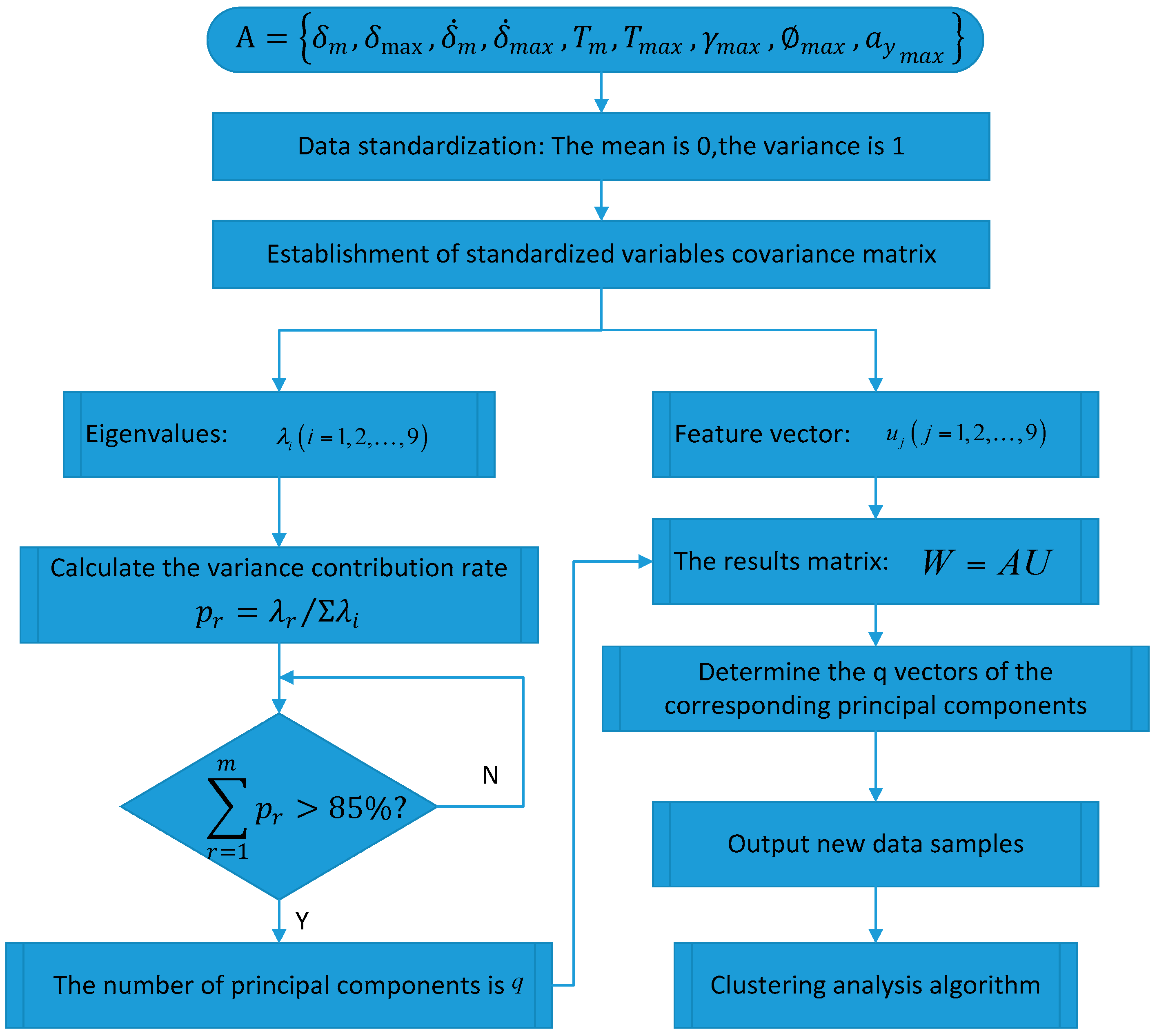
Y9	0.005	0.04	100

. According to the principal component analysis principle, the first four principal components are selected, and the correlation between the characteristic parameters and the principal components is analyzed. The representative average angular velocity, average steering angle, maximum yaw rate and maximum lateral acceleration, the four parameters of acceleration, are used for cluster analysis. The method of principal component analysis is shown in Figure 10.

5. Comparison of Clustering Analysis Methods

5.1. Fuzzy C-Means Algorithm

The fuzzy C-means clustering is defined as:

$$\overline{J}\left(X;U,V,\lambda \right)={\displaystyle \sum _{i=1}^c{\displaystyle \sum _{k=1}^N{\left({\mu }_{ik}\right)}^m}}{D}_{ikA}^2+{\displaystyle \sum _{k=1}^N{\lambda }_k}\left({\displaystyle \sum _{i=1}^c{\mu }_{ik}-1}\right)$$

(4)

and by setting the gradients of ($\overline{J}$) with respect to U, V and $\lambda$ to zero. If $D_{ikA}^2$ > 0, $\forall i$, k and m > 1, then $\left(U,V\right)\in M_{fc}\times R^{n\times c}$ may minimize only if:

$${\mu }_{ik}=\frac{1}{{{\displaystyle \sum {}_{j=1}^c\left(D_{ikA}/D_{jkA}\right)}}^{2/\left(m-1\right)}},1\le i\le c,1\le k\le N$$

(5)

Additionally:

$$v_i=\frac{{\displaystyle \sum _{k=1}^N{\mu }_{ik}^m}{x}_k}{{\displaystyle \sum _{k=1}^N{\mu }_{ik}^m}},1\le i\le c$$

(6)

5.2. Gustafson–Kessel Algorithm

The Gustafson–Kessel algorithm obtains the objective function by introducing the covariance matrix, which is suitable for the clustering analysis of the correlation between the variables and is suitable for the distribution of irregular data [32]. The clustering algorithm uses the adaptive distance of the clustering covariance matrix to measure. By obtaining the objective function to achieve the membership matrix of the fuzzy clustering, , and the clustering center $V={\left(v_1,v_2,v_3,\cdots ,v_c\right)}^T$, where: c is the number of samples; $u_{ij}$ is the clustering center membership relative to the data point; and they meet $u_{ij}\in [0,1]$, ${\displaystyle \sum _{i=1}^c{u}_{ij}=1}$, $1\le j\le N$. The data sequence $X=\left(x_1,x_2,\cdots ,x_N\right)$ is given, and its minimized objective function is:

$$J\left(X,V,U\right)={\displaystyle \sum _{i=1}^c{\displaystyle \sum _{j=1}^N\left(u_{ij}\right)}}{}^m{D}_{ij}^2$$

(7)

$$D_{ij}^2={\Vert x_j-v_i\Vert }_{A_i}^2={\left(x_j-v_i\right)}^T{A}_i\left(x_j-v_i\right)$$

(8)

$$A_i=\det {\left(F_i\right)}^{\frac{1}{n}}{F}_i^{-1}$$

(9)

where: m is the fuzzy index, representing the degree of fuzzy clustering, and the greater the value of m, the greater the degree of overlap between the major clusters; usually, m takes one or two; $D_{ij}^2$ is the distance from any data point $x_j$ to the cluster center $v_i$, and it is a square inner product norm; $A_i$ is a positive definite symmetric matrix, and it is determined by the clustering matrix covariance matrix $F_i$.

However, Formula (9) cannot be minimized directly considering its linear features. In order to obtain a viable solution, A_i must be constrained in some way. The usual way is to constrain the determinant of A_i. The allowable matrix A_i varies with its determinant, corresponding to the shape of the optimized cluster, while its volume remains unchanged:

$$\Vert A_i\Vert ={\rho }_i,\rho >0$$

(10)

where ${\rho }_i$ is certain for each cluster. Using the Lagrange multiplier method, A_i is obtained:

$$A_i={\left[{\rho }_i\det \left(F_i\right)\right]}^{1/n}{F}_i^{-1}$$

(11)

where F_i is defined by:

$$F_i=\frac{{\displaystyle \sum _{k=1}^N{\left({\mu }_{ik}\right)}^m}\left(x_k-v_i\right){\left(x_k-v_i\right)}^T}{{\displaystyle \sum _{k=1}^N{\left({\mu }_{ik}\right)}^m}}$$

(12)

5.3. Gath–Geva Algorithm

The Gath–Geva algorithm was proposed by Bezdek and Dunn [33]:

$$D_{ik}\left(x_k,v_i\right)=\frac{\sqrt{\det \left(F_{\omega i}\right)}}{{\alpha }_i}\exp \left(\frac{1}{2}{\left(x_k-v_i{}^{\left(l\right)}\right)}^T{F}_{\omega i}^{-1}\left(x_k-v_i{}^{\left(l\right)}\right)\right)$$

(13)

The difference between the GG algorithm and the GK algorithm is that the distance norm involves an exponential term. $F_{\omega i}$ is the fuzzy covariance matrix of the i-th cluster, given by:

$$F_{\omega i}=\frac{{\displaystyle \sum _{k=1}^N{({\mu }_{ik})}^{\omega }}\left(x_k-v_i\right){\left(x_k-v_i\right)}^T}{{\displaystyle \sum _{k=1}^N{({\mu }_{ik})}^{\omega }}},1\le i\le c$$

(14)

The prior probabilities formula for each classification are given by:

$${\alpha }_i=\frac{1}{N}{\displaystyle \sum _{k=1}^N{\mu }_{ik}}$$

(15)

6. Clustering Results and Analysis

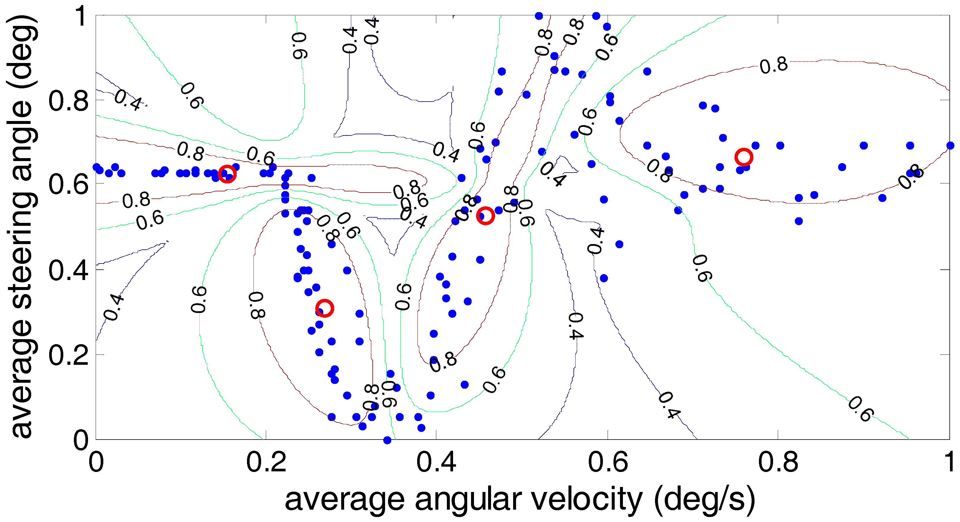
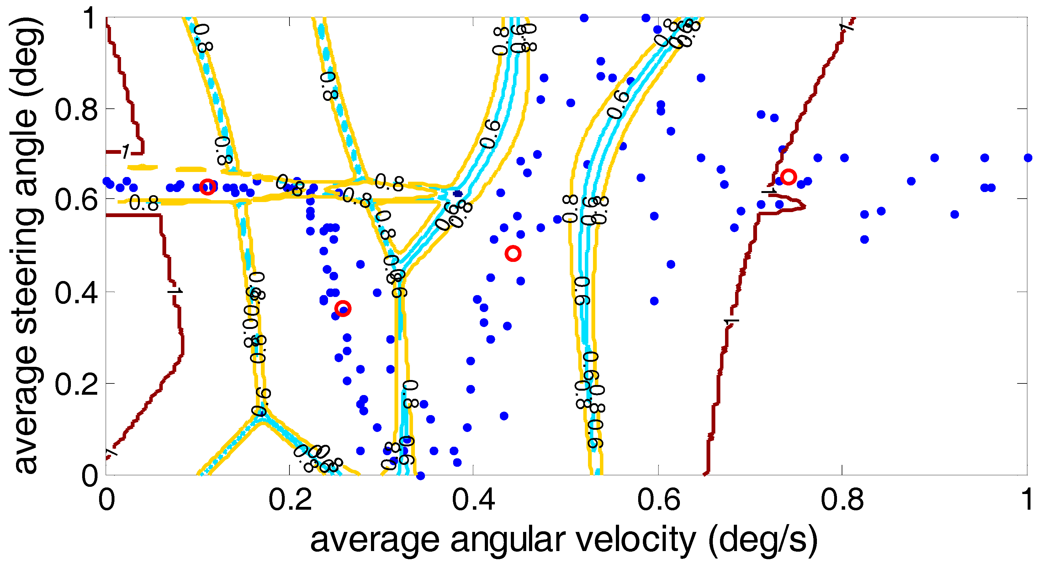
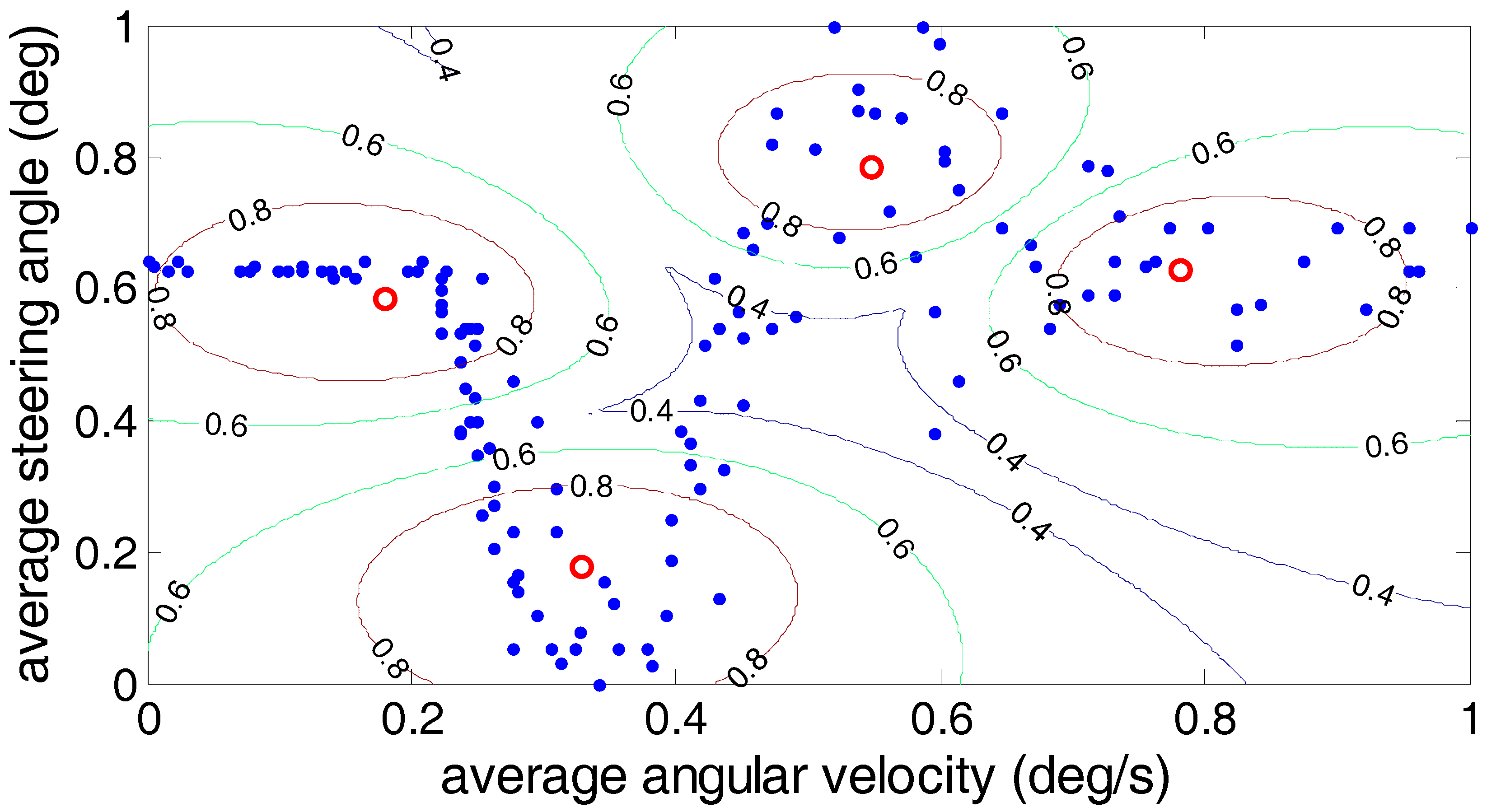
In order to further analyze the driver’s steering characteristics under the steering conditions after clustering, the results are shown by the average angular velocity and the average steering angle. As shown in Figure 11, Figure 12 and Figure 13, the fuzzy C-means algorithm, the Gustafson–Kessel algorithm and the Gath–Geva algorithm were used to divide the driver’s steering test results into four classes, and in each algorithm, the cluster center for each class is marked. (0.18, 0.59), (0.33, 0.18), (0.55, 0.785) and (0.785, 0.625) are the four clustering centers given by the fuzzy C-means algorithm; the Gustafson–Kessel algorithm gives four clustering centers: (0.155, 0.62), (0.27, 0.305), (0.46, 0.53) and (0.76, 0.67). The four cluster centers (0.115, 0.63), (0.255, 0.365), (0.44, 0.48) and (0.742, 0.649) are given by the Gath–Geva algorithm. According to the fourth cluster center, we can see that the average angular velocity and the average steering angle of the drivers’ steering are larger. This reflects the driver’s steering intention under the U-turn condition. Analysis of the first and second cluster centers revealed that these two types of conditions exist; the lower average angular velocity and larger average steering angle. It can be judged at this time that the first cluster reflects the drivers’ steering intention under the lane change condition, and the second cluster centers reflects drivers’ steering intention under the lane keeping condition. The remaining third cluster center between the fourth and first two cluster centers usually belongs to the ordinary driver’s intentions for the turn right/left steering conditions.

Three kinds of clustering analysis methods can be used to separate the experimental data under different steering conditions into four different types. However, by comparing the three clustering methods, we can find that for the third cluster center, the average steering angle is greater than the average steering angle of the center of the fourth cluster using the fuzzy C-means algorithm, which is contrary to the fact that the average steering angle under the normal right/left turn is less than the average steering angle of the U-turn. Therefore, the accuracy of the Gustafson–Kessel algorithm and the Gath–Geva algorithm is superior to the fuzzy C-means algorithm.

In order to analyze the clustering effect more scientifically, in the clustering method, the most representative criteria for evaluating the clustering effect are the Partition Coefficient (PC) and the Classification Entropy (CE), which are defined as follows:

The Partition Coefficient (PC) measures the amount of “overlapping” between clusters. It is defined by Bezdek as follows:

$$PC (c)=\frac{1}{N}{\displaystyle \sum _{i=1}^c{\displaystyle \sum _{j=1}^N{({\mu }_{ij})}^2}}$$

(16)

The Classification Entropy (CE) measures the fuzziness of the cluster partition only, which is similar to the partition coefficient.

$$CE (c)=-\frac{1}{N}{\displaystyle \sum _{i=1}^c{\displaystyle \sum _{j=1}^N{\mu }_{ij}\log ({\mu }_{ij})}}$$

(17)

In this paper, C is the number of clusters and N is the total number of experiments. When the two validity evaluation functions reach the optimal value, that is PC (c) reaches the maximum value and CE (c) reaches the minimum value, the clustering analysis effect is better. The comparisons of PC (c) and CE (c) and the required time among different clustering algorithms under different working conditions are shown in

Table 5. Recorded data of the evaluation in three ways.

Algorithm	PC (c)	CE (c)	Time Consumed (s)
Fuzzy C-means	0.6935	0.6096	5.1685
Gustafson–Kessel	0.7356	0.4892	5.7304
Gath–Geva	0.9493	0.0377	5.5268

.

By analyzing

Table 6. The results of the identification.

Distances	Condition 1	Condition 2	Condition 3	Condition 4	Condition 5
The distance to Clustering Center 1	3.4	2.3	0.28	2.8	3.64
The distance to Clustering Center 2	6.8	6.1	4.03	0.65	7.39
The distance to Clustering Center 3	0.25	0.74	2.79	2.7	5.71
The distance to Clustering Center 4	2.2	3.0	4.99	2.47	0.16
The result of identification	Clustering 3	Clustering 3	Clustering 1	Clustering 2	Clustering 4

, we can see that the Gath–Geva algorithm achieves the maximum value for the Partition Coefficient (PC). At the same time, the Gath–Geva algorithm achieves the minimum value for the Classification Entropy (CE). Due to the complexity of the Gath–Geva algorithm, the time consumed area is somewhat more than the fuzzy C-means, but it is also within acceptable limits. To sum up, the Gath–Geva algorithm is better than the other two methods for the classification and identification of driver’s intention.

7. The Results of the Identification of Driver’s Steering Intention

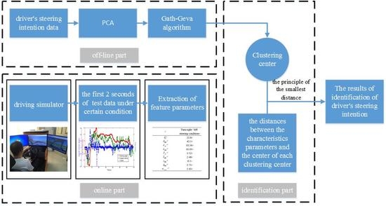
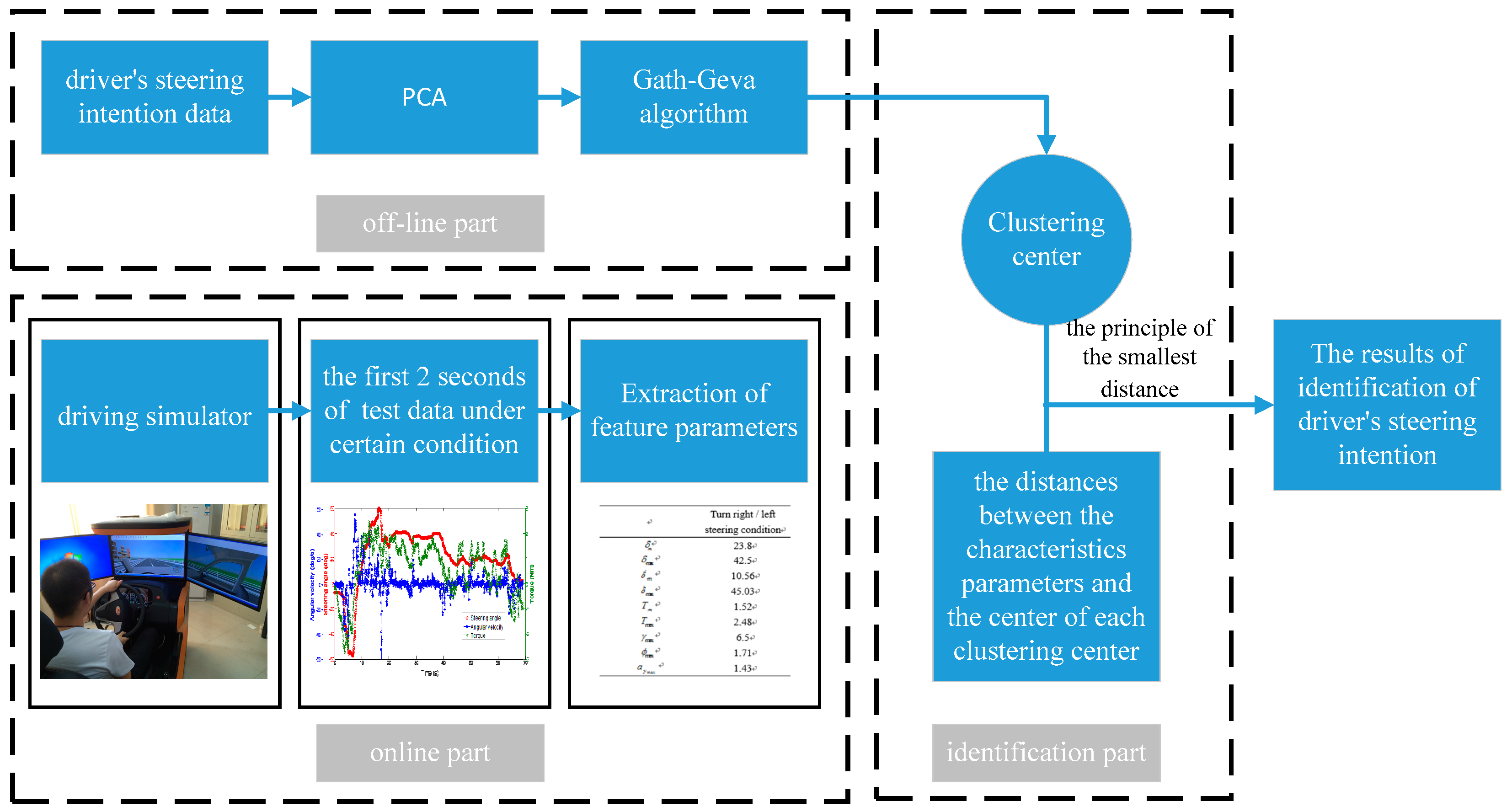
The identification process of the driver’s steering intention is shown in Figure 14 by the method of principal component analysis and the Gath–Geva algorithm, including the offline part, online part and identification. The offline part is to analyze the driver’s steering intention data under different steering conditions through the principal component analysis and Gath–Geva algorithm analysis and get the clustering center. The online and identification parts are the processes of the real-time identification of the driver’s steering intention. Firstly, the first 2 s of the test data are obtained under a certain condition in the driving simulator. Secondly, the characteristics of the data parameters are extracted, and then, the distances between the characteristic parameters and the center of each clustering center are calculated. Finally, according to the principle of the smallest distance, the driver’s steering intention is determined. The distance calculation formula is:

$$d_i=\Vert x-c_i\Vert ,i=1,2,3,4$$

(18)

where x represents the characteristic parameters of one condition, $x=\left(x_1,x_2,\cdots ,x_p\right)$; $c_i$ represents the clustering center parameters for clustering, $c_i=\left(c_{i1},c_{i2},\cdots ,c_{ip}\right)$.

In order to verify the validity of the identification method designed by this article, five different drivers were selected. Five tests were carried out on the driving simulator, namely turning right, turning left, lane changing, lane keeping and U-turn condition. (0.45, 0.65), (0.44, 0.48) and (0.742, 0.649) are given by the Gath–Geva algorithm according to the above, respectively representing lane changing, lane keeping, turning right and U-turn condition. As shown in Table 6, in Conditions 1–5, the distances between the characteristic parameters and the center of each clustering center were calculated. It is shown that the results of each identification are exactly the same as the actual driver’s intention. Therefore, the effectiveness of the identification method designed by this article is verified.

8. Conclusions

In this paper, driver’s characteristic steering parameters under different conditions were proposed. Real vehicle tests under four kinds of typical operating conditions were implemented by five excellent driving school coaches with different ages and genders. The test vehicles covered four different countries’ passenger cars. Then, the principal component analysis and clustering analysis were combined to classify and identify the driver’s steering intention. By comparison and analysis, the Gath–Geva algorithm was significantly better than the other two clustering algorithms under different typical operating conditions to classify and identify the driver’s steering intention. In order to verify the validity of the identification method designed by this article, five different drivers were selected. Five tests were carried out on the driving simulator. It was show that the results of each identification were exactly the same as the actual driver’s intention. Therefore, the effectiveness of the identification method designed by this article was verified.

References

1. Sun, Y.; Xiong, G.G.; Chen, H.Y. Evaluation of Intelligent Behavior of Unmanned Vehicles Based on Fuzzy-EAHP. Automot. Eng. 2014, 36, 22–27. [Google Scholar]
2. Sai, S. Current and future ITS. IEICE Trans. Inf. Syst. 2013, 96, 176–183. [Google Scholar] [CrossRef]
3. Mueller, C.; Siedersberger, K.H.; Faerber, B. Active roll motion as feedback for decoupled steering interventions in Advanced Driver Assistance Systems (ADAS). Forsch. Ingenieurwesn 2017, 81, 41–55. [Google Scholar]
4. Anaya, J.J.; Ponz, A.; Garcia, F. Motorcycle detection for ADAS through camera and V2V Communication, a comparative analysis of two modern technologies. Expert Syst. Appl. 2017, 77, 148–159. [Google Scholar] [CrossRef]
5. Zhao, R.C.; Wong, P.K.; Xie, Z.C. Real-time weighted multi-objective model predictive controller for adaptive cruise control systems. Int. J. Automot. Technol. 2017, 18, 279–292. [Google Scholar] [CrossRef]
6. Li, S.B.; Guo, Q.Q.; Xin, L. Fuel-Saving Servo-Loop Control for an Adaptive Cruise Control System of Road Vehicles with Step-Gear Transmission. IEEE Trans. Veh. Technol. 2017, 66, 2033–2043. [Google Scholar] [CrossRef]
7. Zheng, B.; Anwar, S. Yaw stability control of a steer-by-wire equipped vehicle via active front wheel steering. Mechatronics 2009, 19, 799–804. [Google Scholar] [CrossRef]
8. Sun, X.D.; Chen, L.; Jiang, H.B.; Yang, Z.B.; Chen, J.C.; Zhang, W.Y. High-performance control for a bearingless permanent magnet synchronous motor using neural network inverse scheme plus internal model controllers. IEEE Trans. Ind. Electron. 2016, 63, 3479–3488. [Google Scholar] [CrossRef]
9. Sun, X.D.; Shi, Z.; Chen, L.; Yang, Z.B. Internal model control for a bearingless permanent magnet synchronous motor based on inverse system method. IEEE T. Energy Convers. 2016, 31, 1539–1548. [Google Scholar] [CrossRef]
10. Sun, X.D.; Su, B.K.; Chen, L.; Yang, Z.B.; Xu, X.; Shi, Z. Precise control of a four degree-of-freedom permanent magnet biased active magnetic bearing system in a magnetically suspended direct-driven spindle using neural network inverse scheme. Mech. Syst. Signal Process. 2017, 88, 36–48. [Google Scholar] [CrossRef]
11. Cheng, L.; Qiao, T.Z. Localization in the Parking Lot by Parked-Vehicle Assistance. IEEE Trans. Intell. Transp. 2016, 17, 3629–3634. [Google Scholar] [CrossRef]
12. Sun, X.D.; Chen, L.; Yang, Z.B. Overview of bearingless permanent magnet synchronous motors. IEEE Trans. Ind. Electron. 2013, 60, 5528–5538. [Google Scholar] [CrossRef]
13. Cheon, D.S.; Nam, K.H. Steering torque control using variable impedance models for a steer-by-wire system. Int. J. Automot. Technol. 2017, 18, 263–270. [Google Scholar] [CrossRef]
14. Kim, W.H.; Son, Y.S.; Chung, C.C. Torque-Overlay-Based Robust Steering Wheel Angle Control of Electrical Power Steering for a Lane-Keeping System of Automated Vehicles. IEEE Trans. Veh. Technol. 2016, 65, 4379–4392. [Google Scholar] [CrossRef]
15. Sun, X.D.; Chen, L.; Yang, Z.B.; Zhu, H.Q. Speed-sensorless vector control of a bearingless induction motor with artificial neural network inverse speed observer. IEEE ASME Trans. Mech. 2013, 18, 1357–1366. [Google Scholar] [CrossRef]
16. Windridge, D.; Shaukat, A.; Hollnagel, E. Characterizing Driver Intention via Hierarchical Perception-Action Modeling. IEEE Trans. Hum. Mach. Syst. 2013, 43, 17–31. [Google Scholar] [CrossRef]
17. Li, L.; Zhu, Z.B.; Wang, X.Y. Identification of a driver’s starting intention based on an artificial neural network for vehicles equipped with an automated manual transmission. Proc. Inst. Mech. Eng. D J. Automob. 2016, 230, 1417–1429. [Google Scholar] [CrossRef]
18. Takano, W.; Matsushita, A.; Iwao, K. Recognition of human driving behaviors based on stochastic symbolization of time series signal. In Proceedings of the IEEE/RSJ International Conference on Intelligent Robots and Systems, Nice, France, 22–26 September 2008; pp. 167–172. [Google Scholar]
19. Raksin, C.P.; Mizushima, T.; Nagai, M. Direct yaw moment control system based on driver behavior recognition. Veh. Syst. Dyn. 2008, 46, 911–921. [Google Scholar]
20. Tesheng, H. Time-varying system identificationvia maximum a posteriori estimation and its application to driver steering models. In Proceedings of the American Control Conference, Westin Seattle Hotel, Seattle, WA, USA, 11–13 June 2008; pp. 11–13. [Google Scholar]
21. Harmouche, J. Incipient fault detection and diagnosis based on Kullback Leibler divergence using PCA: Part I. Signal Process. 2014, 94, 278–287. [Google Scholar] [CrossRef]
22. Nguyen, T.H.; Kim, H. Novel and efficient pedestrian detection using bidirectional PCA. Pattern Recogn. 2013, 46, 2220–2227. [Google Scholar] [CrossRef]
23. Ding, M. Adaptive KPCA. Signal Process. 2010, 90, 1542–1553. [Google Scholar] [CrossRef]
24. Zhou, K.; Yang, S. Exploring the uniform effect of FCM clustering: A data distribution perspective. Knowl. Based Syst. 2016, 96, 76–83. [Google Scholar] [CrossRef]
25. Andrea, B.; Palma, B. A survey of fuzzy clustering algorithms for pattern recognition I. IEEE Trans. Syst. Man. Cybern. Soc. 1999, 29, 778–785. [Google Scholar]
26. Zarita, Z.; Pauline, O. Design of wavelet neural networks based on symmetry fuzzy c-means for function approximation. Neural Comput. Appl. 2013, 23, 247–259. [Google Scholar]
27. Zhou, D.G.; Zhou, H. A modified strategy of fuzzy clustering algorithm for image segmentation. Soft Comput. 2015, 19, 3261–3272. [Google Scholar] [CrossRef]
28. Saber, S.; Selamat, A.; Fujita, H. Systematic mapping study on granular computting. Knowl. Based Syst. 2015, 80, 78–97. [Google Scholar]
29. Abonyi, J.; Babuska, R.; Szeifert, F. Modified Gath-Geva fuzzy clustering for identification of Takagi-Sugeno fuzzy models. IEEE Trans. Syst. Man Cybern. B 2002, 32, 612–621. [Google Scholar] [CrossRef] [PubMed]
30. Sarbu, C.; Zehl, K.; Einax, J.W. Fuzzy divisive hierarchical clustering of soil data using Gustafson-Kessel algorithm. Chemom. Intell. Lab. 2007, 86, 121–129. [Google Scholar] [CrossRef]
31. Price, A.L.; Patterson, N.J.; Plenge, R.M. Principal components analysis corrects for stratification in genome-wide association studies. Nat. Genet. 2006, 38, 904–909. [Google Scholar] [CrossRef] [PubMed]
32. Gustafson, D.E.; Kessel, W.C. Fuzzy clustering with fuzzy covariance matrix. In Proceedings of the 1978 IEEE Conference on Decision and Control including the 17th Symposium on Adaptive Processes, San Diego, CA, USA, 10–12 January 1979; pp. 761–766. [Google Scholar]
33. Bezdek, J.C. Pattern Recognition with Fuzzy Objective Function Algorithms; Plenum Press: New York, NY, USA, 1981. [Google Scholar]
Figure 1. Experimental devices and the actual installation.
Applsci 07 01014 g001
Figure 2. Experimental vehicles (1) GM GL8, (2) Skoda Octavia, (3) Honda Accord, (4) SAIC MG.
Applsci 07 01014 g002
Figure 3. Filter results with the Butterworth filter: (a) torque; (b) angular velocity; (c) yaw rate; and (d) lateral acceleration.
Applsci 07 01014 g003aApplsci 07 01014 g003b
Figure 4. Steering angle under different steering conditions: (a) turning right; (b) U-turn; (c) lane keeping; (d) lane changing.
Applsci 07 01014 g004
Figure 5. Angular velocity under different steering conditions: (a) turning right; (b) U-turn; (c) lane keeping; (d) lane changing.
Applsci 07 01014 g005aApplsci 07 01014 g005b
Figure 6. Torque under different steering conditions: (a) turning right; (b) U-turn; (c) lane keeping; (d) lane changing.
Applsci 07 01014 g006
Figure 7. Roll angle under different steering conditions: (a) turning right; (b) U-turn; (c) lane keeping; (d) lane changing.
Applsci 07 01014 g007aApplsci 07 01014 g007b
Figure 8. Lateral acceleration under different steering conditions: (a) turning right; (b) U-turn; (c) lane keeping; (d) lane changing.
Applsci 07 01014 g008
Figure 9. Yaw rate under different steering conditions: (a) turning right; (b) U-turn; (c) lane keeping; (d) lane changing.
Applsci 07 01014 g009aApplsci 07 01014 g009b
Figure 10. Method of principal component analysis.
Applsci 07 01014 g010
Figure 11. Visualization of the classification results of the driver’s steering intention based on the fuzzy C-means algorithm.
Applsci 07 01014 g011
Figure 12. Visualization of the classification results of the driver’s steering intention based on the Gustafson–Kessel algorithm.
Applsci 07 01014 g012
Figure 13. Visualization of the classification results of the driver’s steering intention based on the Gath–Geva algorithm.
Applsci 07 01014 g013
Figure 14. The flowchart for the identification of the driver’s steering intention. PCA: Principal Component Analysis.
Applsci 07 01014 g014