Investigation of Heat Loss from the Finned Housing of the Electric Motor of a Vacuum Pump


Abstract
:1. Introduction
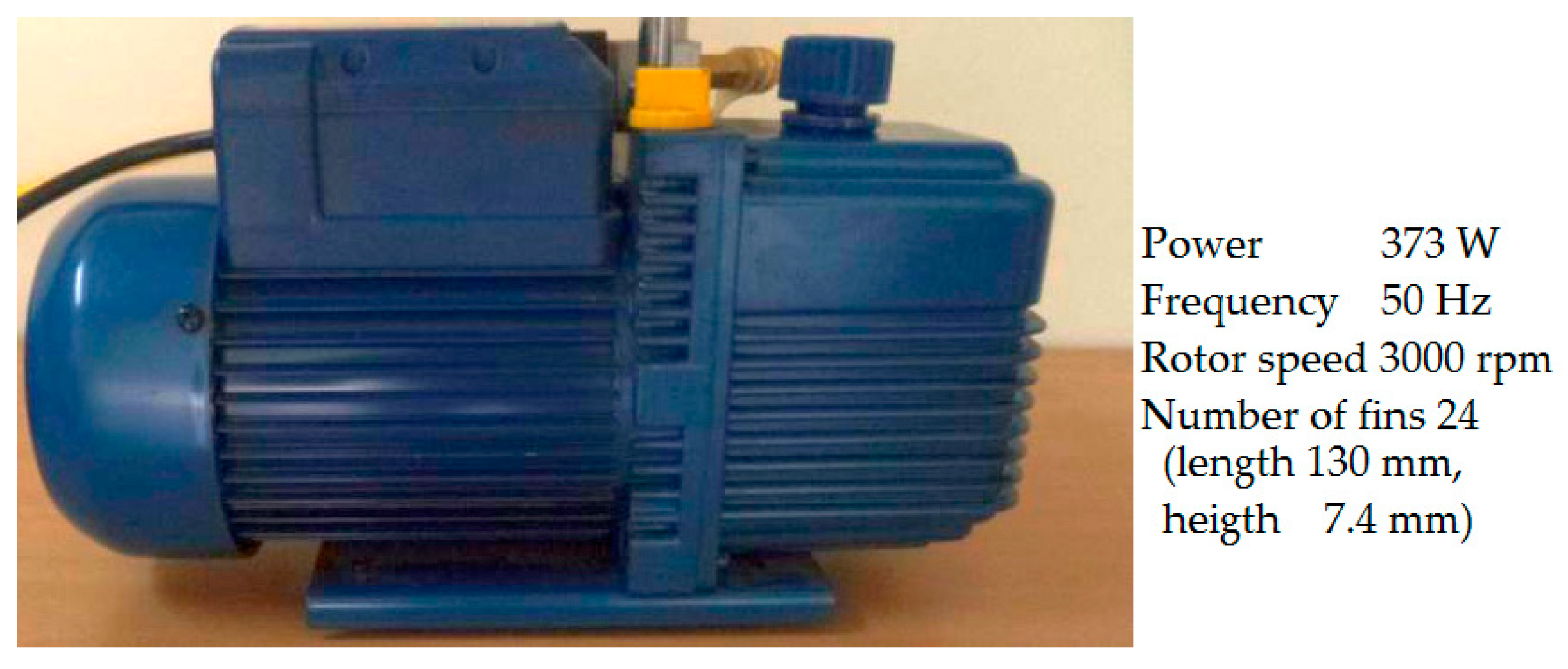
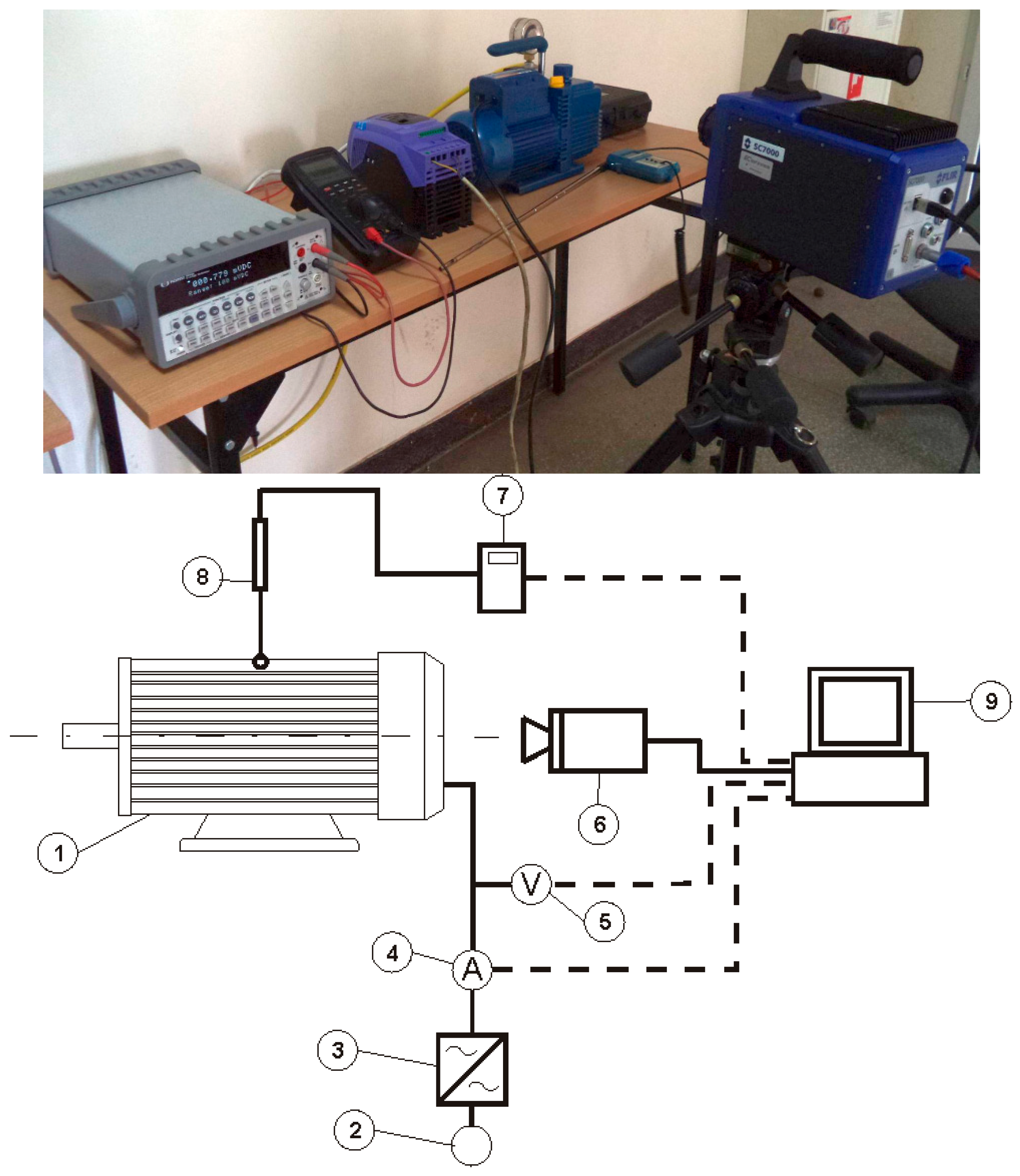
2. Methodology
3. Results and Discussion
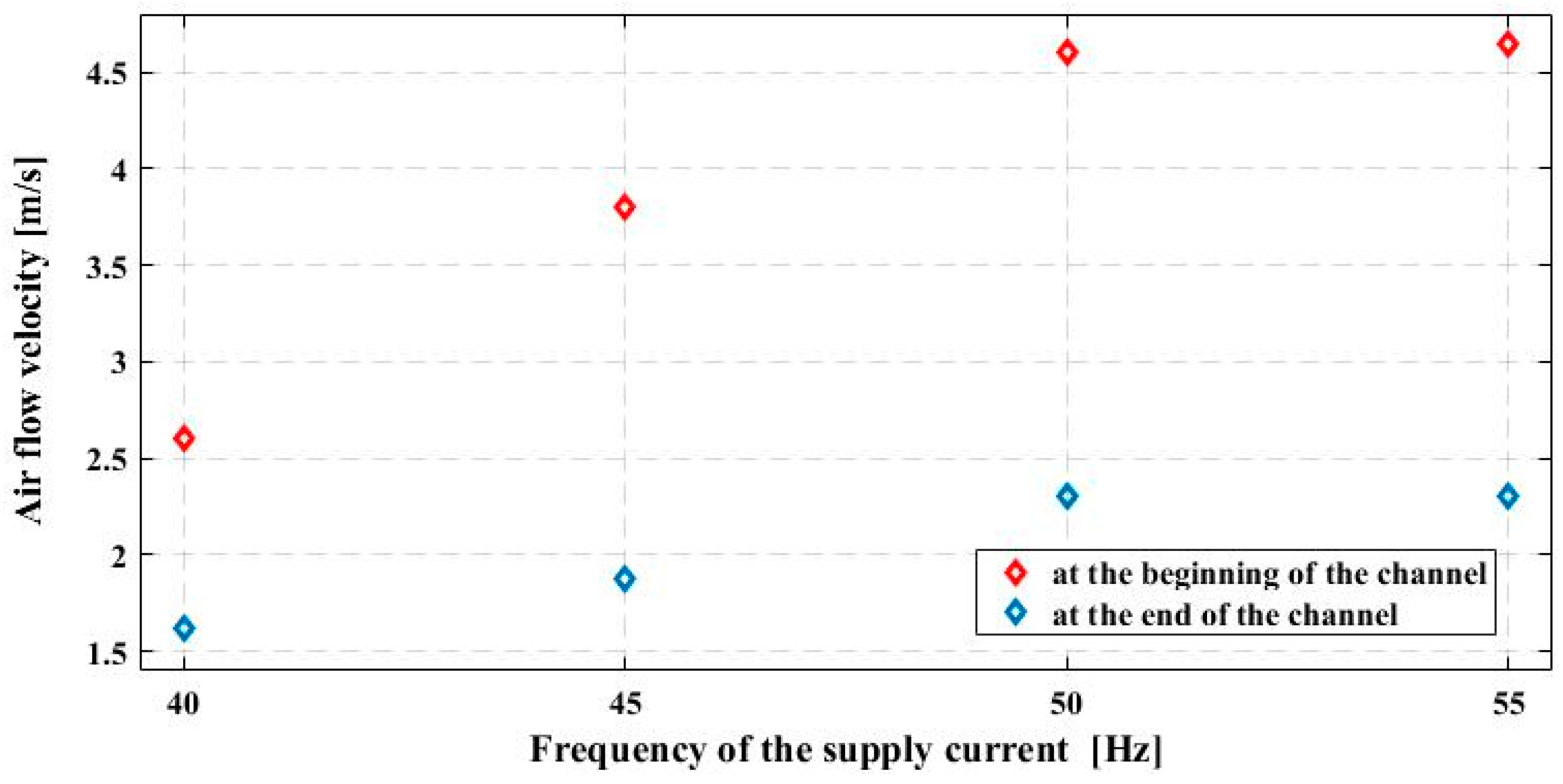
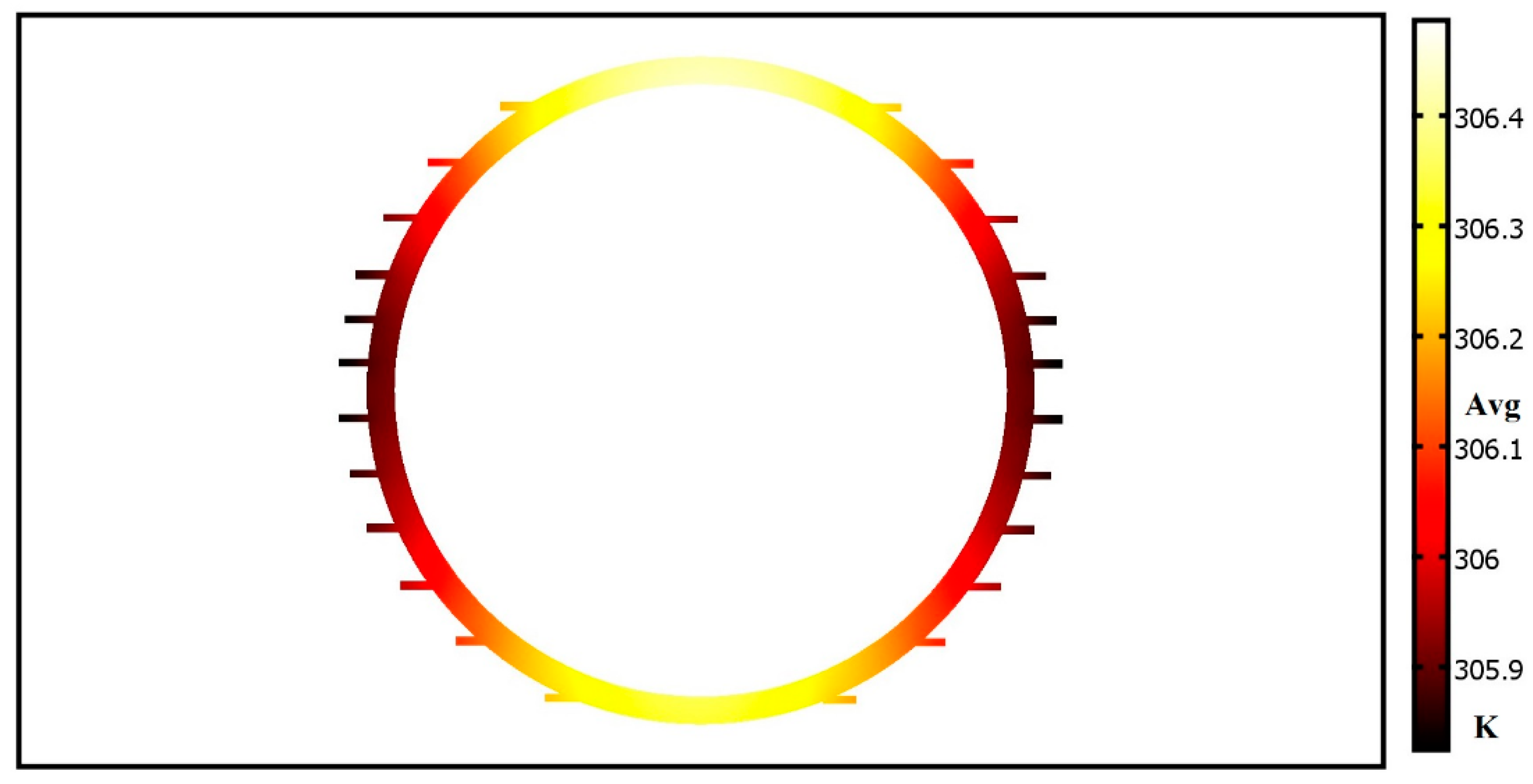
3.1. Measured Operating Parameters
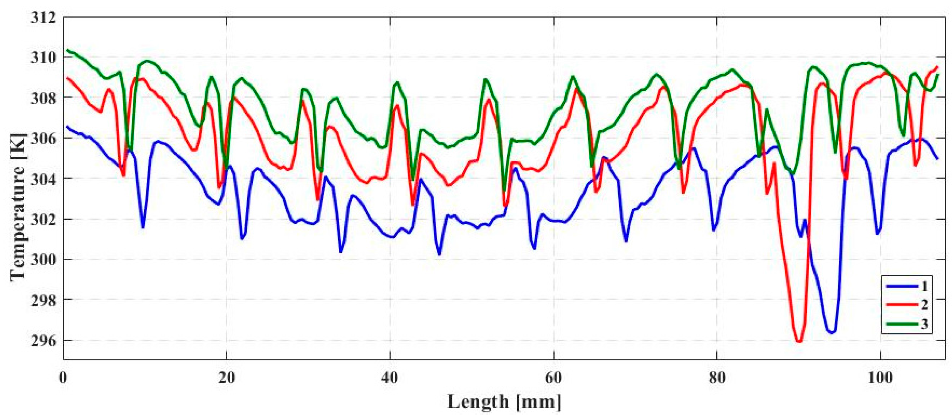
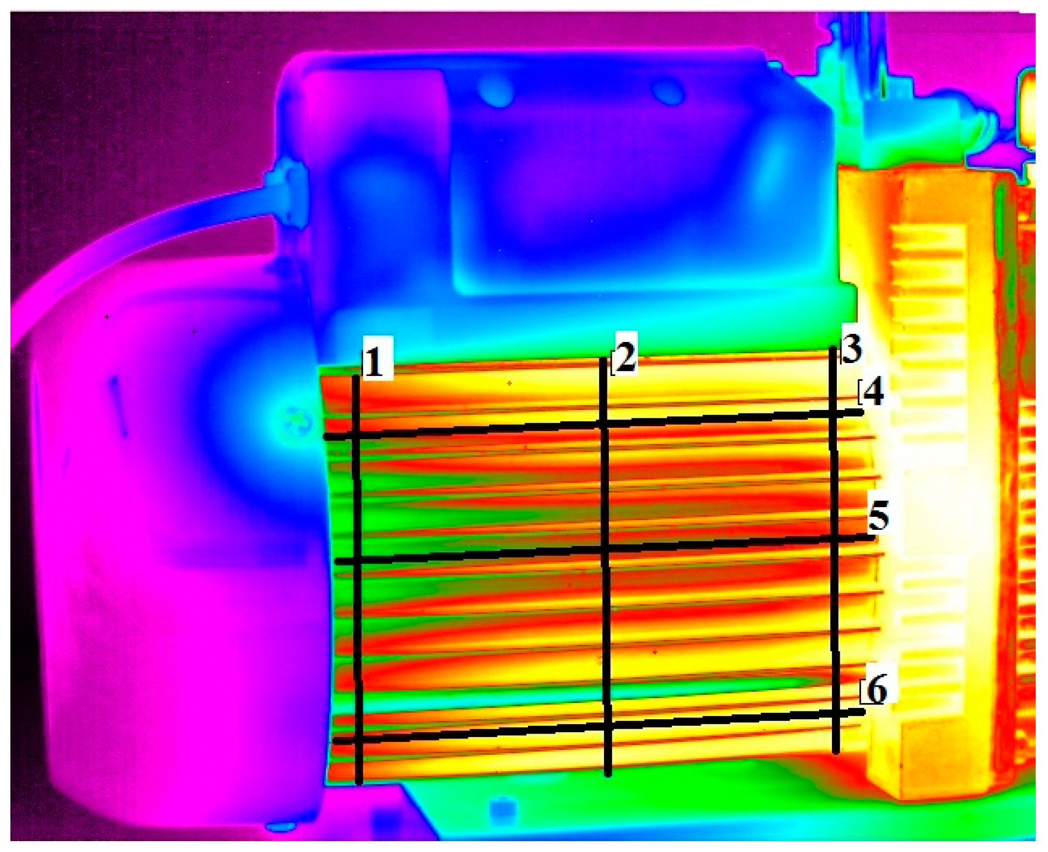
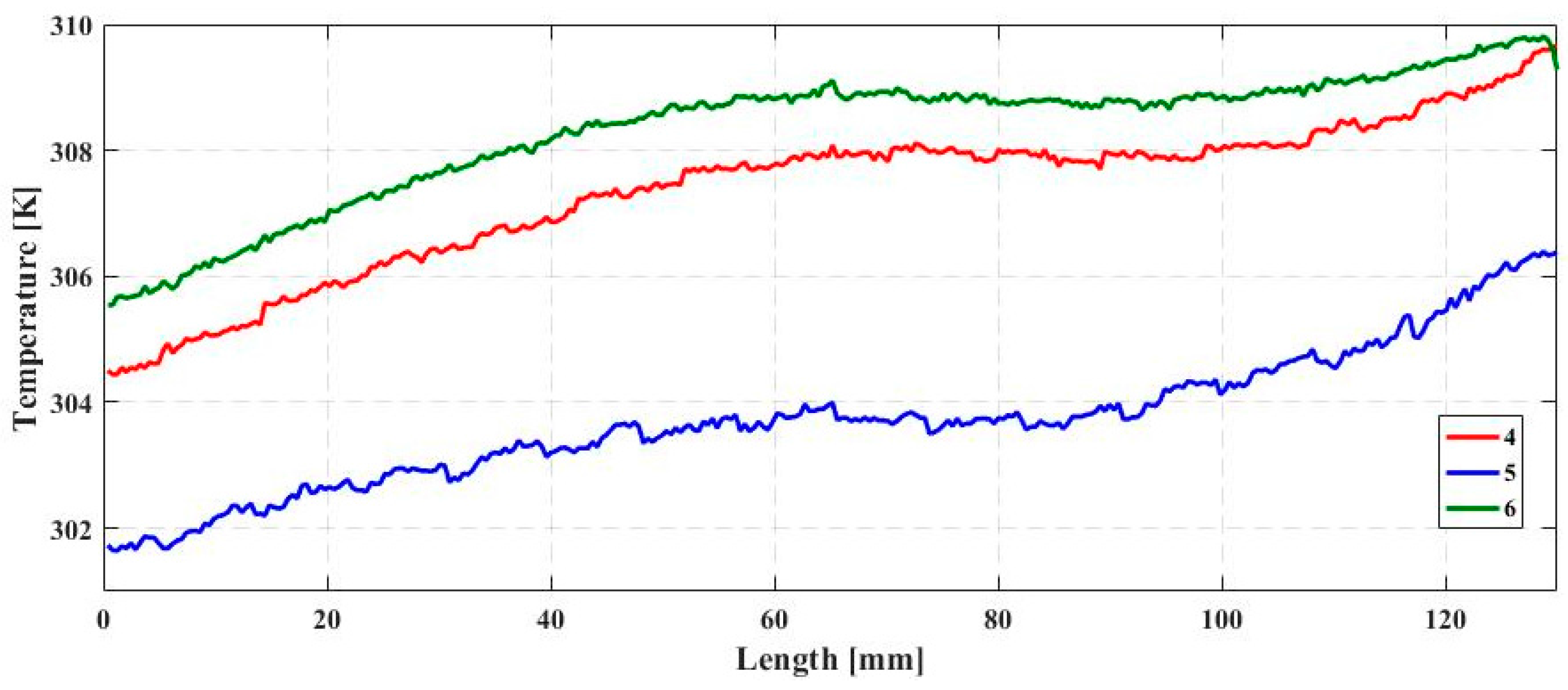
3.2. Thermographical Investigation
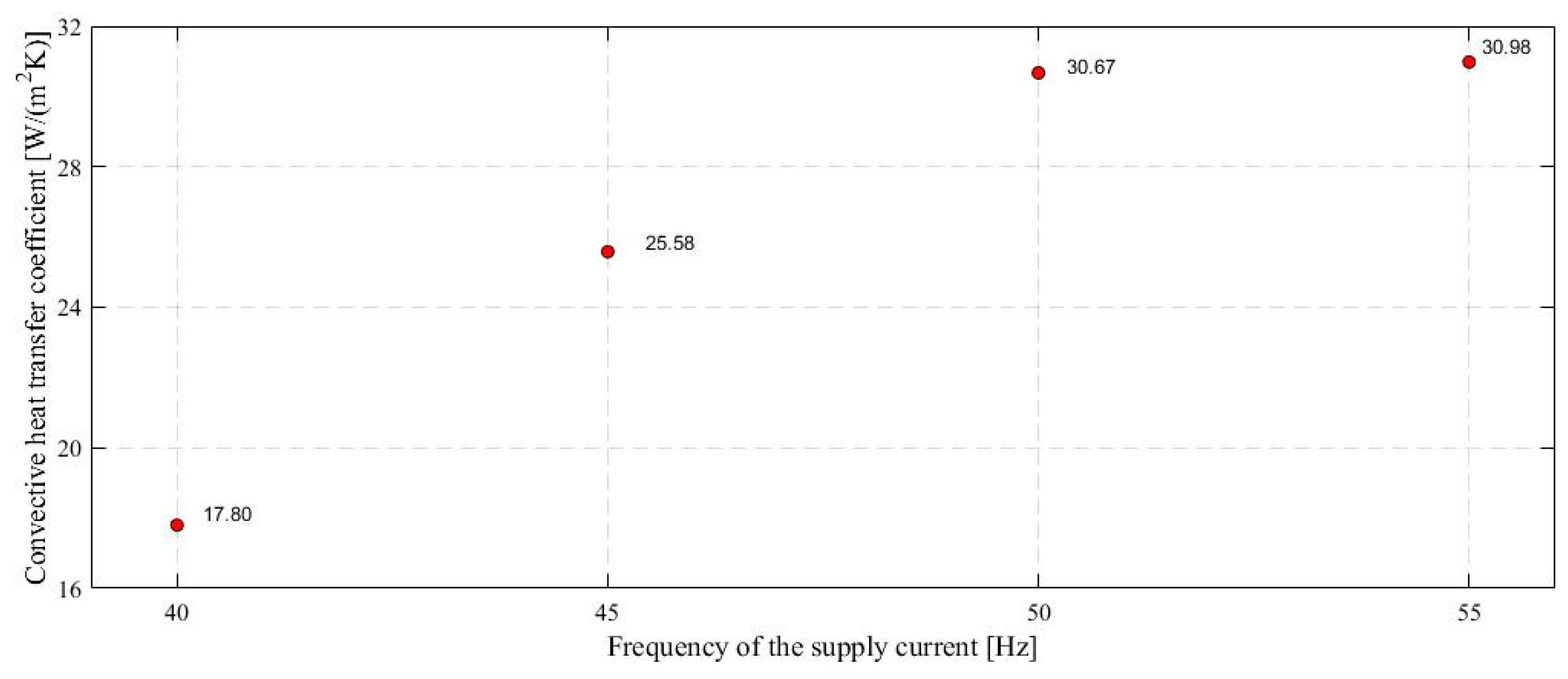
3.3. Convective Heat Transfer Coefficients
3.4. Numerical Simulations
- -
- thermal conductivity for aluminum: 180 W/(mK),
- -
- ambient temperature: 295 K,
- -
- external housing surface exposed to the ambient air is cooled by forced convection described by the expression:where, n—unit vector normal to the studied surface, Tf—ambient temperature.
4. Conclusions
Conflicts of Interest
References
- Da Costa Bortoni, E. Are my motors oversized? Energy Convers. Manag. 2009, 50, 2282–2287. [Google Scholar] [CrossRef]
- Aziz, A.; Bouaziz, M.N. A least squares method for a longitudinal fin with temperature dependent internal heat generation and thermal conductivity. Energy Convers. Manag. 2011, 52, 2876–2882. [Google Scholar] [CrossRef]
- Xie, Y.; Wang, Y. 3D temperature field analysis of the induction motors with broken bar fault. Appl. Therm. Eng. 2014, 66, 25–34. [Google Scholar] [CrossRef]
- Pyrhönen, J.; Lindh, P.; Polikarpova, M.; Kurvinen, E.; Naumanen, V. Heat-transfer improvements in an axial-flux permanent-magnet synchronous machine. Appl. Therm. Eng. 2015, 76, 245–251. [Google Scholar] [CrossRef]
- Liu, G.R.; Quek, S.S. The Finite Element Method; Butterworth-Heinemann: Oxford, UK, 2014. [Google Scholar] [CrossRef]
- Baskharone, E.A. The Finite Element Method with Heat Transfer and Fluid Mechanics Applications; Cambridge University Press: New York, NY, USA, 2014. [Google Scholar]
- Moradnia, P.; Golubev, M.; Chernoray, V.; Nilsson, H. Flow of cooling air in an electric generator model—An experimental and numerical study. Appl. Energy 2014, 114, 644–653. [Google Scholar] [CrossRef]
- Tosetti, M.; Maggiore, P.; Cavagnino, A.; Vaschetto, S. Conjugate heat transfer analysis of integrated brushless generators for more electric engines. IEEE Trans. Ind. Appl. 2014, 50, 2467–2475. [Google Scholar] [CrossRef]
- Klimenta, D.; Hannukainen, A. Novel approach to analytical modelling of steady-state heat transfer from the exterior of TEFC induction motors. Therm. Sci. 2016, 21, 1529–1542. [Google Scholar] [CrossRef]
- Krajačić, G.; Duić, N.; Rosen, M.A. Sustainable development of energy, water and environment systems. Energy Convers. Manag. 2015, 125, 1–14. [Google Scholar] [CrossRef]
- Yong, J.Y.; Klemeš, J.J.; Varbanov, P.S.; Huisingh, D. Cleaner energy for cleaner production: Modelling, simulation, optimisation and waste management. J. Clean. Prod. 2016, 111, 1–16. [Google Scholar] [CrossRef]
- Romo, J.L.; Adrián, M.B. Prediction of internal temperature in three-phase induction motors with electronic speed control. Electr. Power Syst. Res. 1998, 45, 91–99. [Google Scholar] [CrossRef]
- Wrobel, R.; Vainel, G.; Copeland, C.; Duda, T.; Staton, D.; Mellor, P.H. Investigation of Mechanical Loss Components and Heat Transfer in an Axial-Flux PM Machine. IEEE Trans. Ind. Appl. 2015, 51, 3000–3011. [Google Scholar] [CrossRef]
- Grabowski, M.; Urbaniec, K.; Wernik, J.; Wołosz, K.J. Numerical simulation and experimental verification of heat transfer from a finned housing of an electric motor. Energy Convers. Manag. 2016, 125, 91–96. [Google Scholar] [CrossRef]
- FLIR Systems, User’s Manual I3,I5,I7, T559580; FLIR: Wilsonville, OR, USA, 2011.
- Staton, D.A.; Cavagnino, A. Convection heat transfer and flow calculations suitable for electric machines thermal models. IEEE Trans. Ind. Electron. 2008, 55, 3509–3516. [Google Scholar] [CrossRef]
- Pryor, R. Multiphysics Modeling Using COMSOL 5 and MATLAB; Mercury Learning & Information: Dulles, VA, USA, 2016. [Google Scholar]
- Oberkampf, W.L.; Trucano, T.G. Verification and validation benchmarks. Nucl. Eng. Des. 2008, 238, 716–743. [Google Scholar] [CrossRef]
- Ho, S.L.; Fu, W.N. Analysis of indirect temperature-rise tests of induction machines using time stepping FEM. IEEE Trans. Energy Convers. 2001, 16, 55–60. [Google Scholar] [CrossRef]


| Frequency of the Supply Current (Hz) | 40 | 45 | 50 | 55 |
|---|---|---|---|---|
| Air flow velocity at the channel beginning/end (m/s) | 2.60/1.62 | 3.80/1.88 | 4.60/2.30 | 4.65/2.30 |
| Power consumed by the motor (W) | 212 | 243 | 249 | 250 |
| Frequency of the Supply Current (Hz) | 40 | 45 | 50 | 55 |
|---|---|---|---|---|
| Average temperature of the housing (K) | 314.05 | 311.43 | 306.10 | 315.42 |
| Frequency of the Supply Current (Hz) | 40 | 45 | 50 | 55 |
|---|---|---|---|---|
| base/head of fin, Tmeasured (K) | 314.60/313.20 | 311.80/310.82 | 306.67/305.90 | 315.04/313.99 |
| base/head of fin, Tsimul (K) | 314.57/313.28 | 311.81/310.91 | 306.64/305.92 | 315.06/313.91 |
| ε% | 9.28 | 8.16 | 6.49 | 9.52 |
© 2017 by the author. Licensee MDPI, Basel, Switzerland. This article is an open access article distributed under the terms and conditions of the Creative Commons Attribution (CC BY) license (http://creativecommons.org/licenses/by/4.0/).
Share and Cite
Wernik, J. Investigation of Heat Loss from the Finned Housing of the Electric Motor of a Vacuum Pump. Appl. Sci. 2017, 7, 1214. https://doi.org/10.3390/app7121214
Wernik J. Investigation of Heat Loss from the Finned Housing of the Electric Motor of a Vacuum Pump. Applied Sciences. 2017; 7(12):1214. https://doi.org/10.3390/app7121214
Chicago/Turabian StyleWernik, Jacek. 2017. "Investigation of Heat Loss from the Finned Housing of the Electric Motor of a Vacuum Pump" Applied Sciences 7, no. 12: 1214. https://doi.org/10.3390/app7121214
APA StyleWernik, J. (2017). Investigation of Heat Loss from the Finned Housing of the Electric Motor of a Vacuum Pump. Applied Sciences, 7(12), 1214. https://doi.org/10.3390/app7121214