
Dynamic Shear Degradation of Geosynthetic–Soil Interface in Waste Landfill Sites


1
Civil and Architectural Engineering Group, Korea District Heating Engineering Co. Ltd., 55 Bundang-ro, Bundang-gu, Sungnam-si, Gyeonggi-do 13591, Korea
2
Department of Civil and Environmental Engineering, Seoul National University, 599 Gwanak-ro, Gwanak-gu, Seoul 08826, Korea
3
Department of Civil Engineering, Hanseo University, 46 Hanseo 1-ro, Haemi-myun, Seosan-si, Chungcheognam-do 31962, Korea
*
Author to whom correspondence should be addressed.
Appl. Sci. 2017, 7(12), 1225; https://doi.org/10.3390/app7121225
Submission received: 17 October 2017
/
Revised: 15 November 2017
/
Accepted: 16 November 2017
/
Published: 27 November 2017
(This article belongs to the Section Mechanical Engineering)
Abstract
:Geosynthetics and soil particles inevitably come into contact, resulting in a geosynthetic–soil interface. The discontinuity of the materials at the interface causes an intricate shear response, especially under dynamic loads. In the present study, the effects of chemical aggressors of the leachate from a waste landfill site on the cyclic shear behaviors of a geosynthetic–soil interface were investigated. The Multi-Purpose Interface Apparatus (M-PIA) that can simulate cyclic simple shear conditions was utilized, and 72 sets of cyclic simple shear tests were conducted. The Disturbed State Concept (DSC) was employed to quantitatively estimate the shear stress degradation. As a result, new disturbance functions and parameters that represent the characteristics of the dynamic shear degradation at the interface were evaluated. Additionally, a numerical back-prediction was performed to verify the accuracy and applicability of the DSC parameters. Numerical interpolation procedures were suggested and enabled to reproduce the degradation successfully. Consequently, a general methodology was established to estimate the cyclic shear stress degradation of the geosynthetic–soil interface in consideration of chemical effects.
1. Introduction
Most of earth structures involve the combination of different materials such as soil, rock, concrete, geosynthetics, etc. due to the diversity of construction areas and materials. The area formed between adjacent materials is called the “interface”. In engineering systems, discontinuities exist at the interface and the overall system shows discontinuous behavior due to the discontinuities. Therefore, the theoretical approaches that are based on continuum mechanics may exhibit limitations for the characterization of the interface response. Further, the difference of the intrinsic material properties at the interface entails complicated problems. With rapid industrialization, the quantity of waste has continuously increased. Waste comprises different forms and may degrade into harmless products, or it may be non-degradable or even hazardous. Worldwide, landfilling is the most popular means of hazardous- and municipal-waste disposal because it can be relatively safe and cost-effective when it is based on a precise design and managed with sufficient care [1]. However, landfills have also been identified as one of the major threats to groundwater resources [2], and hazardous- and municipal-waste landfill facilities therefore require lining and covering systems that are mainly organized by geosynthetics and soils. Various types of geosynthetics with diverse functions such as reinforcement, filtration, drainage, protection, and separation are used in the facilities. These geosynthetic systems are currently an accepted and well-established component of the landfill industry [3], and the geosynthetic–soil interface inevitably appears at waste landfill sites. The interface is comprised in base and side slopes of the waste landfill as shown in Figure 1. Figure 1 displays the brief section of waste landfill and the concept of geosynthetic–soil interface.
An important characteristic of the landfill-liner and -cover systems with respect to stability is the shear resistance along the interface between the various liner- or cover-system components [5]. The shear behaviors of geosynthetics are strongly related to the characteristics of the geosynthetic–soil interface because geosynthetics comprise a self-encompassing interface area that corresponds to conditions such as external forces, friction, and stiffness. Therefore, various studies on the shear behavior of the interface have been performed [6,7,8,9,10]. Ghosh et al. [11,12] proposed a mechanical model to simulate the relationship between the deflection of the soil and the contact pressure at the interface of the double-layer geosynthetic reinforced load transfer platform (LTP) and soft soil, based on analytical approach. The proposed model and parametric studies showed better prediction of LTP behavior. A study of the interface was also developed for soil–structure interaction. Hokmabadi and Fatahi [13] performed a 3-dimensional numerical analysis to investigate the characteristics of soil-structure interaction and its influence on the seismic response of building frames. The interface is modeled as spring–slider systems and it was revealed that the type of foundation is a major contributor to the seismic response of buildings with soil–structure interaction. Nguyen et al. [6] also investigated the soil pile interface-induced effect on pile foundation, based on 3-dimensional numerical analysis. Results showed that the type and size of the pile elements influence the dynamic characteristics and seismic response of the building due to interaction between the soil, pile foundation, and the structure.
Cyclic simple shear tests were performed for the present study in order to investigate the dynamic shear response of the interface, because the seismic stability must be considered in accordance with Article 35 of the Waste Management Enforcement Regulations in Korea. A Multi-Purpose Interface Apparatus (M-PIA) was utilized, and 72 sets of cyclic simple shear tests were performed to investigate the effects of the pH values of the leachate on the shear behavior of the geosynthetic–soil interface. Both the geosynthetics and the soil were submerged in acidic, neutral, and basic solutions for 30 days and 850 days, representing the relatively short-term and long-term behaviors of the interface. The Disturbed State Concept (DSC) and the disturbance function were employed to quantitatively estimate the shear stress degradation based on the experimental study. The convenience and reliability of the DSC were successfully verified in the previous research [14,15,16,17]. Based on the experimental approach, the numerical back-prediction of the cyclic shear stress–strain relationship was accomplished based on the parametric study. The numerical back-prediction results were compared with the experimental data that were obtained using the cyclic simple shear test under the stated chemical conditions in order to verify the accuracy and the applicability of the DSC parameters.
2. Chemical Characteristics of Leachate
The biodegradation of waste and leachate occurs in the presence of oxygen under the effect of aerobic bacteria, in the absence of oxygen under the effect of anaerobic bacteria, or with very little oxygen under the effect of facultative anaerobic bacteria. The quantity of oxygen inside the landfill changes with the progression of the decomposition process. The previous studies reported that the pH value changes dramatically because of the complicated biological and chemical reactions in the leachate [18]. Oweis and Khera [19] reported the pH values of 3.5 pH to 8.5 pH for the leachate from municipal waste landfills, and Bilgili et al. [20] demonstrated the variation of the pH values in a landfill site according to the burial period. Therefore, the geosynthetics and soils in waste landfills are exposed to neutrality, acidity, and basicity [21]. Further, the leachate pH is considered to be the most significant parameter that affects the leachate concentration [22], therefore the pH value of the solution is one of the primary governing factors for the manifestation of leachate characteristics, and it can represent the chemical conditions in the present study. Equation (1) and (2) show the chemical reaction formulations between sand (SiO2) and acidity and basicity, respectively.
SiO2 + 4HF → SiF4 + 2H2O
SiO2 + 2NaOH → Na2SiO3 + H2O
3. Disturbed State Concept (DSC)
The Disturbed State Concept and the disturbance function have been employed in the present study to understand the chemical effects on the interface. The early DSC theory was originated by [23] to characterize the softening behavior of an overconsolidated soil, whereby its behavior in a normally consolidated state was used as the reference state. This initial concept was later developed and unified as the DSC to model the behaviors of a wide range of materials [24]. The disturbance function is a key factor of the DSC, and it quantitatively defines dynamic shear stress degradation. The convenience and reliability of the DSC have been successfully verified by the previous research [14,15,16,17], and the numerical formulation of dynamic interface behavior that was achieved with the DSC is a valuable accomplishment [7]. The details of the DSC and the disturbance function are described in previous papers [21,25]. For the disturbance function theory, can be defined based on the shear stresses of the interface that are from the cyclic simple shear test, as follows:
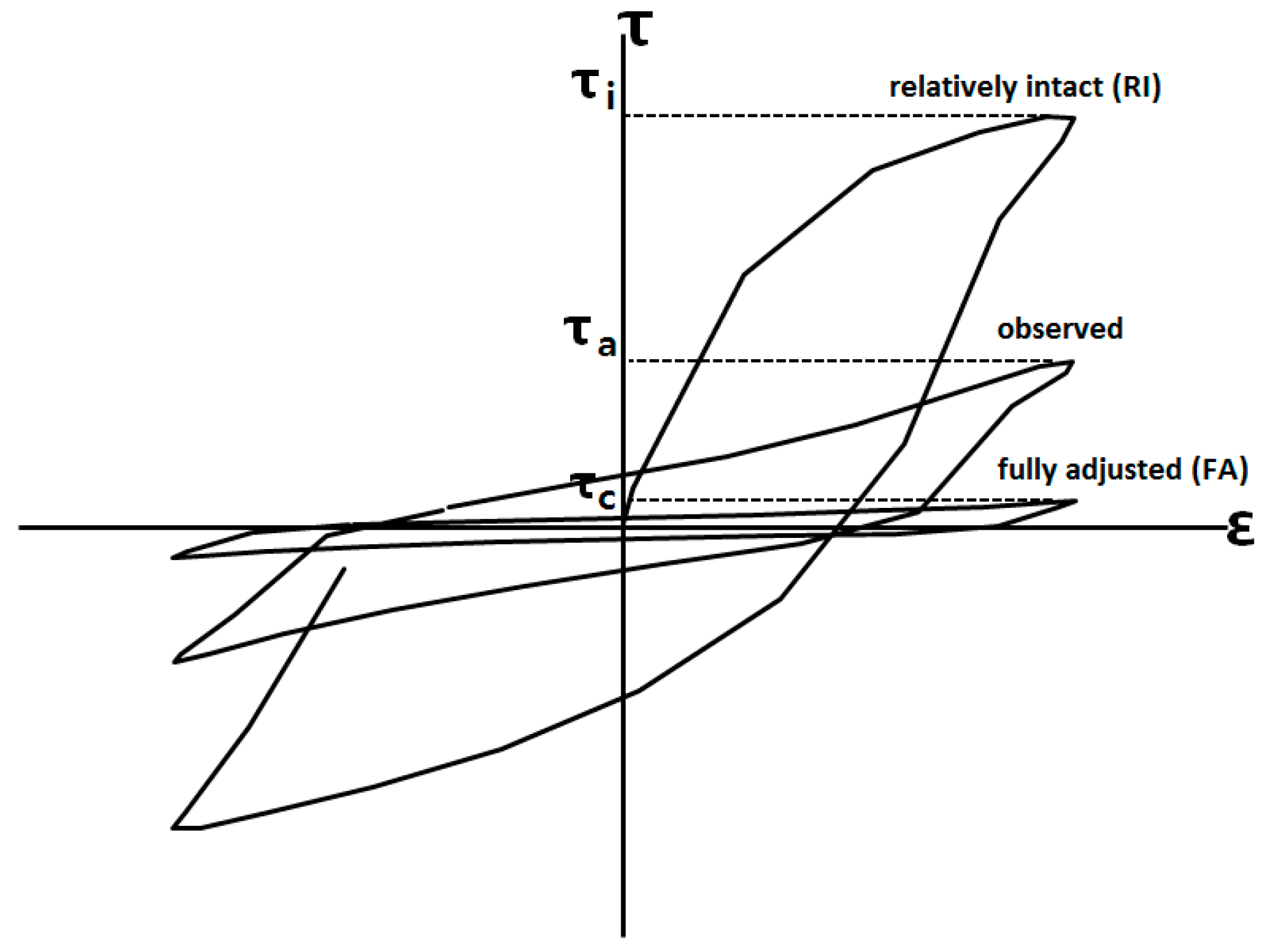
where, a, and c denote the Relatively Intact (RI), observed, and Fully Adjusted (FA) states, respectively. As shown in Figure 2, these values are obtained from the stress–strain curves of the cyclic simple shear test.
The disturbance function can be also expressed as the following equation:
where is the disturbance function value under an FA state and, practically, 0.99 is applicable based on the previous research [26]; and are the intrinsic material parameters that represent the damage growth and the decay processes, respectively [21]; and is the deviatoric plastic strain trajectory that represents the accumulation of the plastic deformation in each cyclic stress–strain loop. Details for estimating the disturbance function and parameters are explained in previous studies [21,25].
4. Laboratory Test
The development of new apparatus and the performance of a few cyclic simple shear tests were accomplished in a previous study [27]. In the present study, 72 sets of cyclic simple shear tests were conducted, and the results of the cyclic simple shear tests are presented and analyzed. Based on the test results, the degree of damage sustained by the geosynthetic–soil interface that was subjected to chemical conditions was quantitatively estimated as a form of the disturbance function curves with newly determined parameters.
4.1. Test Apparatus and Conditions
The Multi-Purpose Interface Apparatus (M-PIA), which was originally manufactured in 2012, and was modified to improve its performance and accuracy in 2015, was utilized to conduct the cyclic simple shear test. Figure 3 describes the outline and the shear-box details of the M-PIA. The structure and technical items are explained in the studies by Kwak et al. [27].
The materials in the test of the geosynthetic–soil interface were the geosynthetics and the granular soil. Jumunjin sand was used in the present study as a typical type of granular soil. The sand specimen was prepared by the air pluviation method at a relative density of 60%. A funnel with a metallic square outlet with a width of 7 mm was used to drop the Jumunjin sand into the shear-box. The sand was spread in the shear-box at a constant speed to a height of 60 cm. The physical characteristics are summarized in Table 1.
A composite type of geosynthetic (i.e., geocomposite) has been most commonly applied to the waste landfill sites of Korea, because it exhibits a strong chemical resistance and superior performance of protection. Table 2 displays the specifications of the geocomposite.
The present study is based on the idea that the chemical aggressor in the leachate that is generated from the decomposition process of the landfill waste will affect the shear behavior of the geosynthetic–soil interface under the monotonic and dynamic-loading conditions. As an antioxidant such as carbon black is added to the manufacturing process for high-density polyethylene (HDPE), it is postulated that soil decay will be the main reason for the shear strength degradation of the geosynthetic–soil interface, rather than damage to the geocomposite. A few studies on the shear strength degradation of the geosynthetic–soil interface under dynamic-loading conditions have been performed [17,29]. Others have studied only the chemical conditions decay of raw materials [30,31]. However, for the present study, the simultaneous occurrence of the chemical effect on the geosynthetic–soil interface and the dynamic-loading conditions were considered. Previous studies have shown that pH values changes dramatically due to the complicated biological and chemical reactions in leachate [20,32]. Therefore, in the present study, the chemical conditions of leachate were incorporated by using buffer solutions of different pH values. Both geosynthetic and soil specimens were submerged in the basic, neutral, and acidic solutions for 30 days and 850 days in order to consider the short- and long-term responses of the interface, respectively.
Considering the unit weight of a waste landfill and the area of the specimen, 0.3 and 0.6 MPa of normal stresses represent heights of 20 and 40 m of landfill waste, respectively. As such, these are the forces that were applied to the specimen. The unit weight of a hazardous waste landfill site is 15.9 to 17.3 kN/m3 [19].
The dynamic conditions were also considered in order to simulate an earthquake load. The predominant frequency range of the earthquake load is between 0.1 Hz and 15 Hz, based on previous studies [33,34]. It is often assumed that soil behavior is independent of the seismic-loading frequencies between 0.1 Hz and 10 Hz. Additionally, ASTM D3999 [35] recommends the frequency of 0.5 Hz or 1.0 Hz in cases where uniform sinusoidal loading is applied. Based on the previous research and recommendation, 0.5 Hz of sinusoidal loading was chosen for the cyclic simple shear test. As such, this study is limited by 0.5 Hz of load conditions and the effect of frequency shall be investigated in a further study. Additionally, a few pilot tests were performed in order to decide the amplitude of the shear strain. If the amplitude was more than 5%, the specimen failed too early, indicating difficulties with regards to the attainment of a sufficient amount of data for an analysis of the shear stress–strain behavior. In the cases of a shear strain below 1.5%, the shear stress–strain curves are too steep and congested to examine. In our tests, many more cycles were required to reach failure under lower shear strain level than 3.0%, or a specimen did not even come to a point of failure under larger shear strain level than 3.0%, therefore, 3.0% of shear strain was applied in the present study. The total numbers of cycles were 200 and 100 for the specimens that were submerged for 30 days and 850 days, respectively. A lower number of cycles was used for the 850-day specimens because a significantly more rapid shear degradation may occur in these specimens.
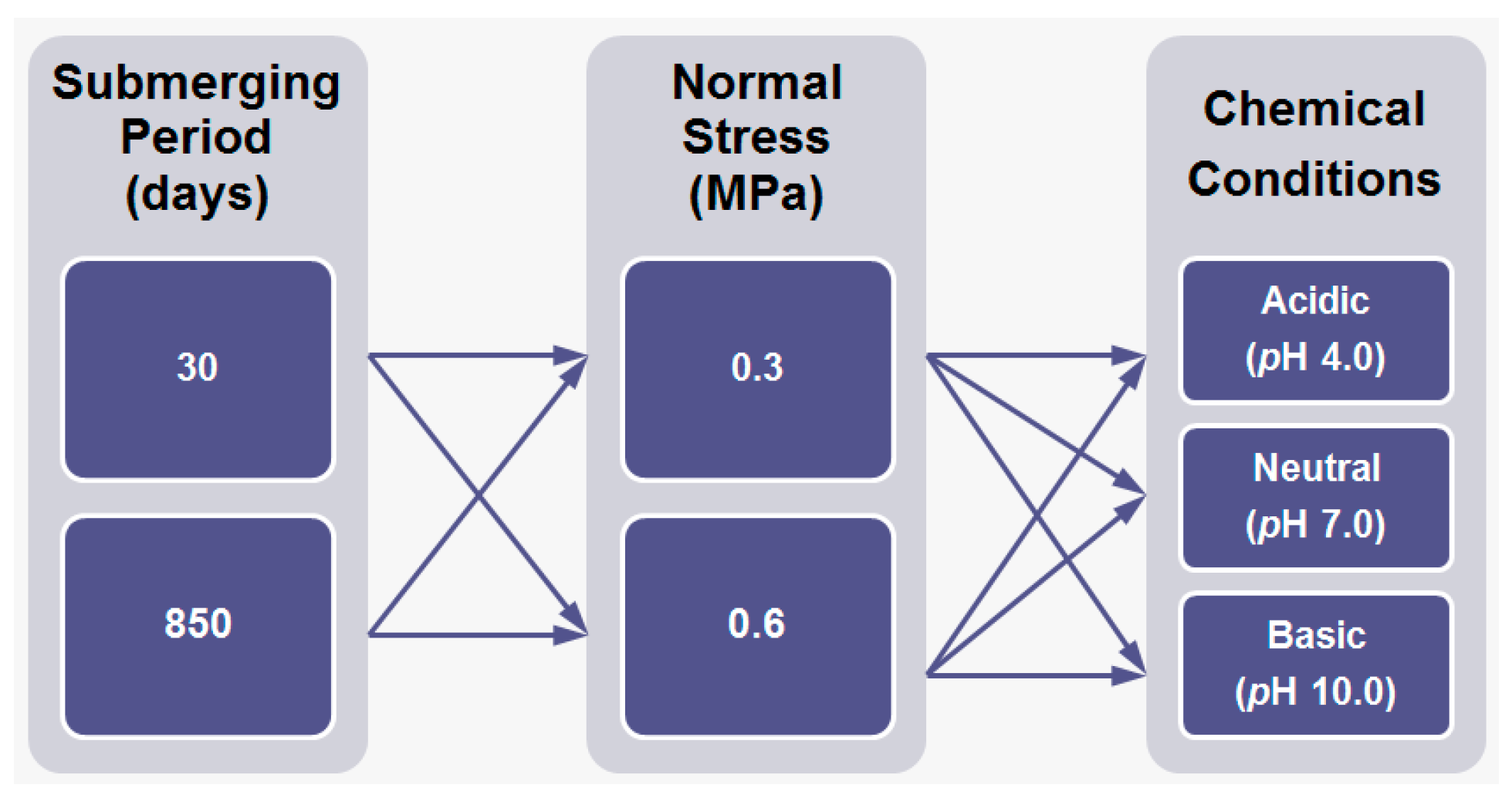
The cyclic simple shear test was conducted six times under each condition; therefore, 72 sets of the test were performed. Figure 4 describes the test schedule for which the chemical and dynamic conditions were considered.
4.2. Test Results
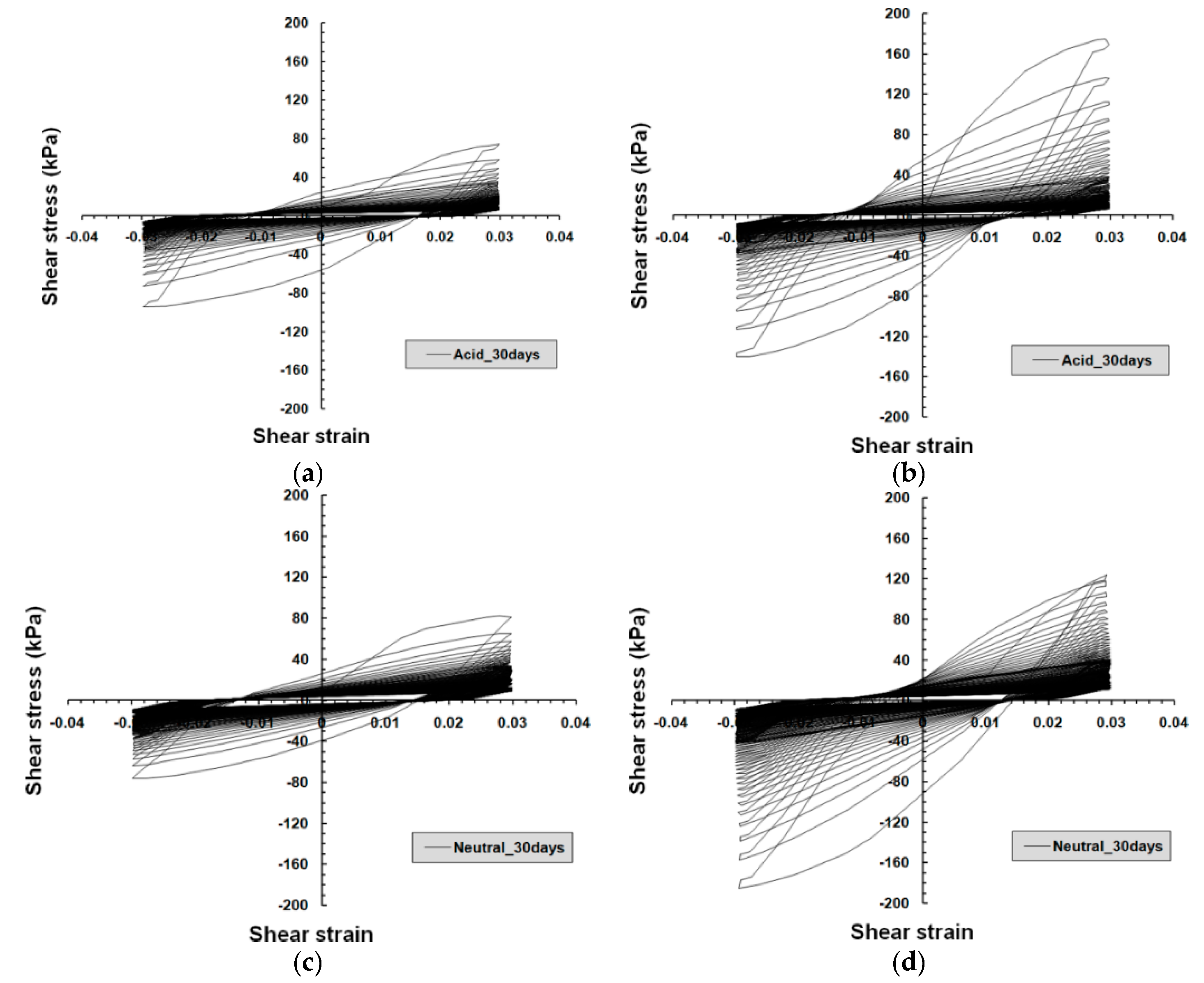
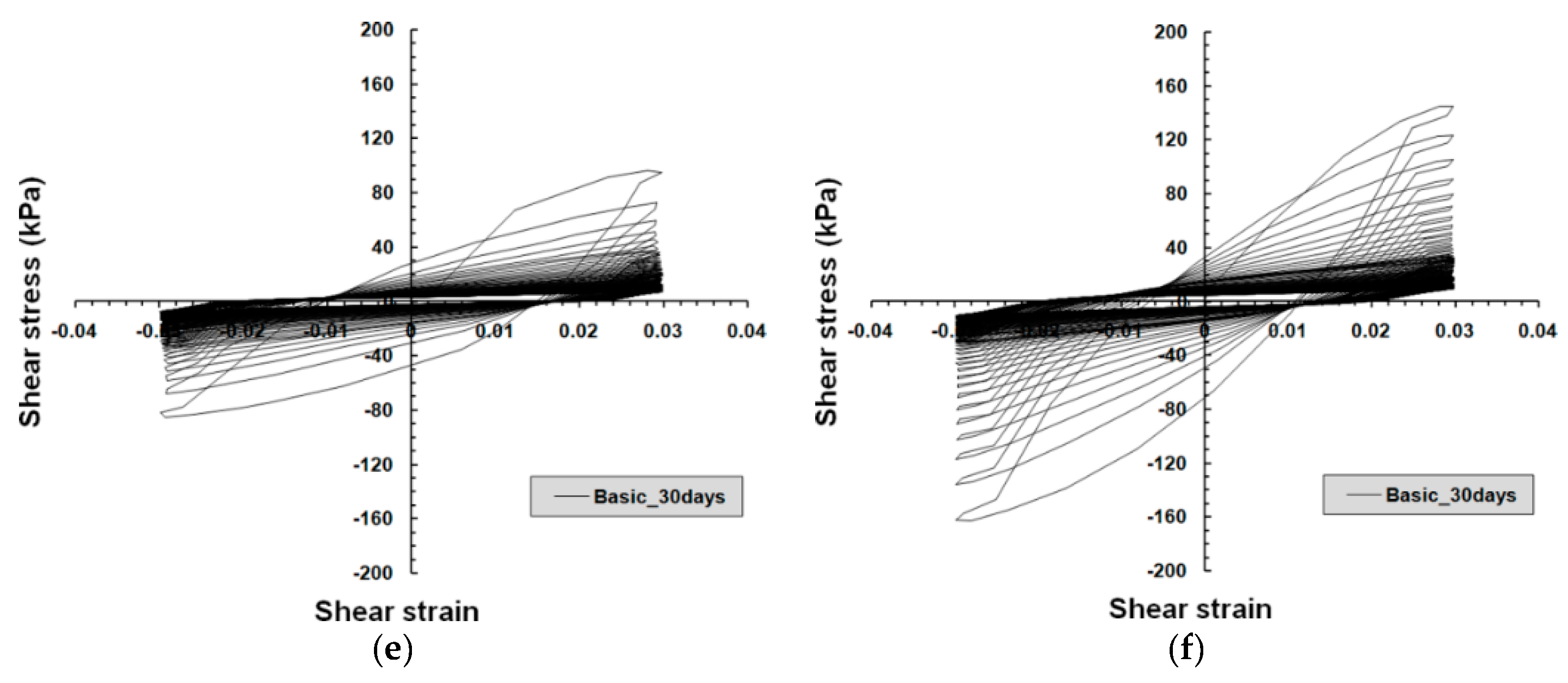
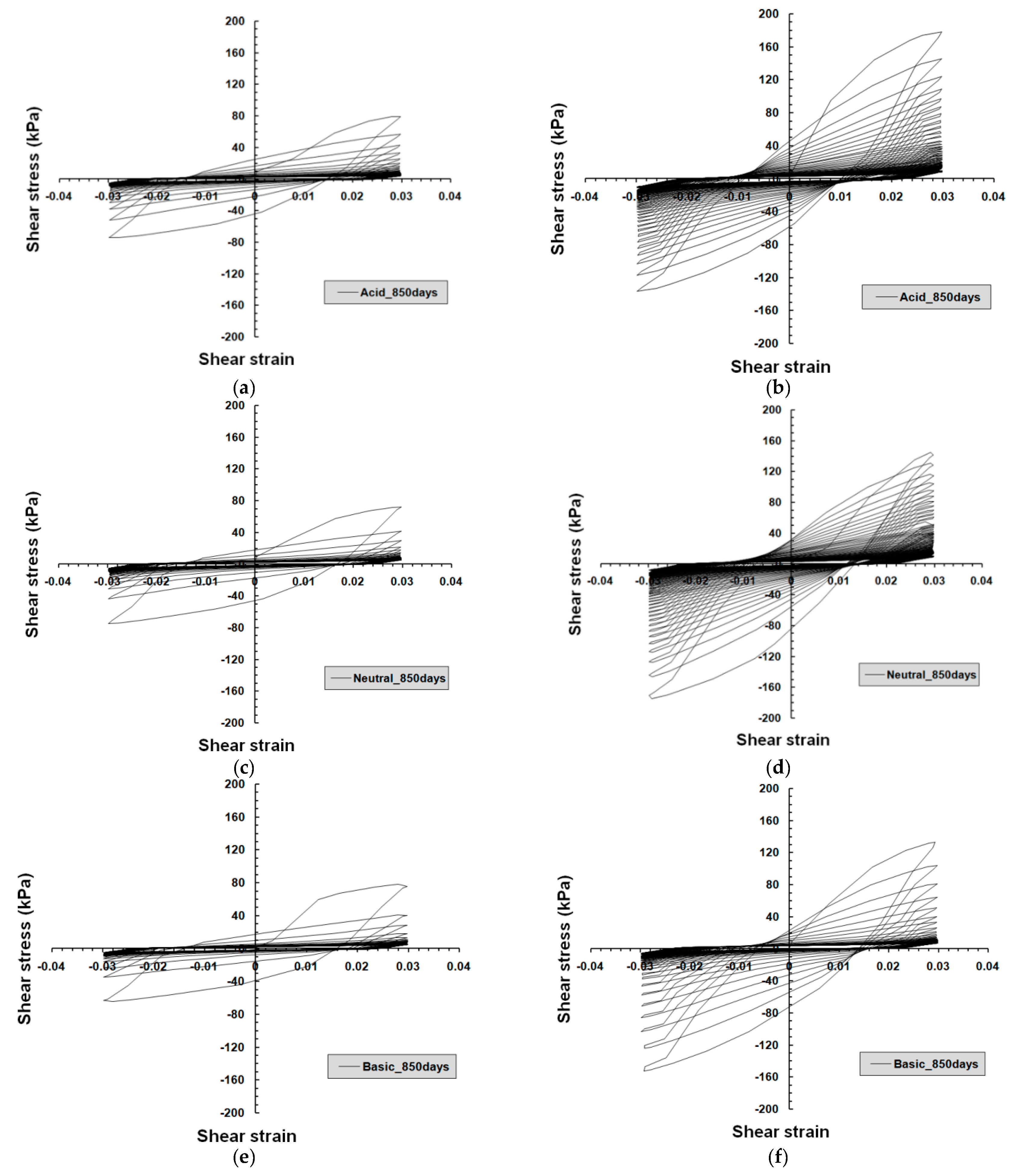
The shear stress–strain curves were obtained from the cyclic simple shear test using the modified M-PIA. Figure 5 and Figure 6 display representative test results of the shear stress–strain relationship for submersion periods of 30 days and 850 days, respectively. An obvious trend of shear stress degradation was observed with an increasing number of load cycles in all of the cases. The rate of the shear degradation tended to decrease with an increase in the number of cycles, but the rate could not be estimated directly yet.
4.3. Evaluation of Disturbance Function and Parameters
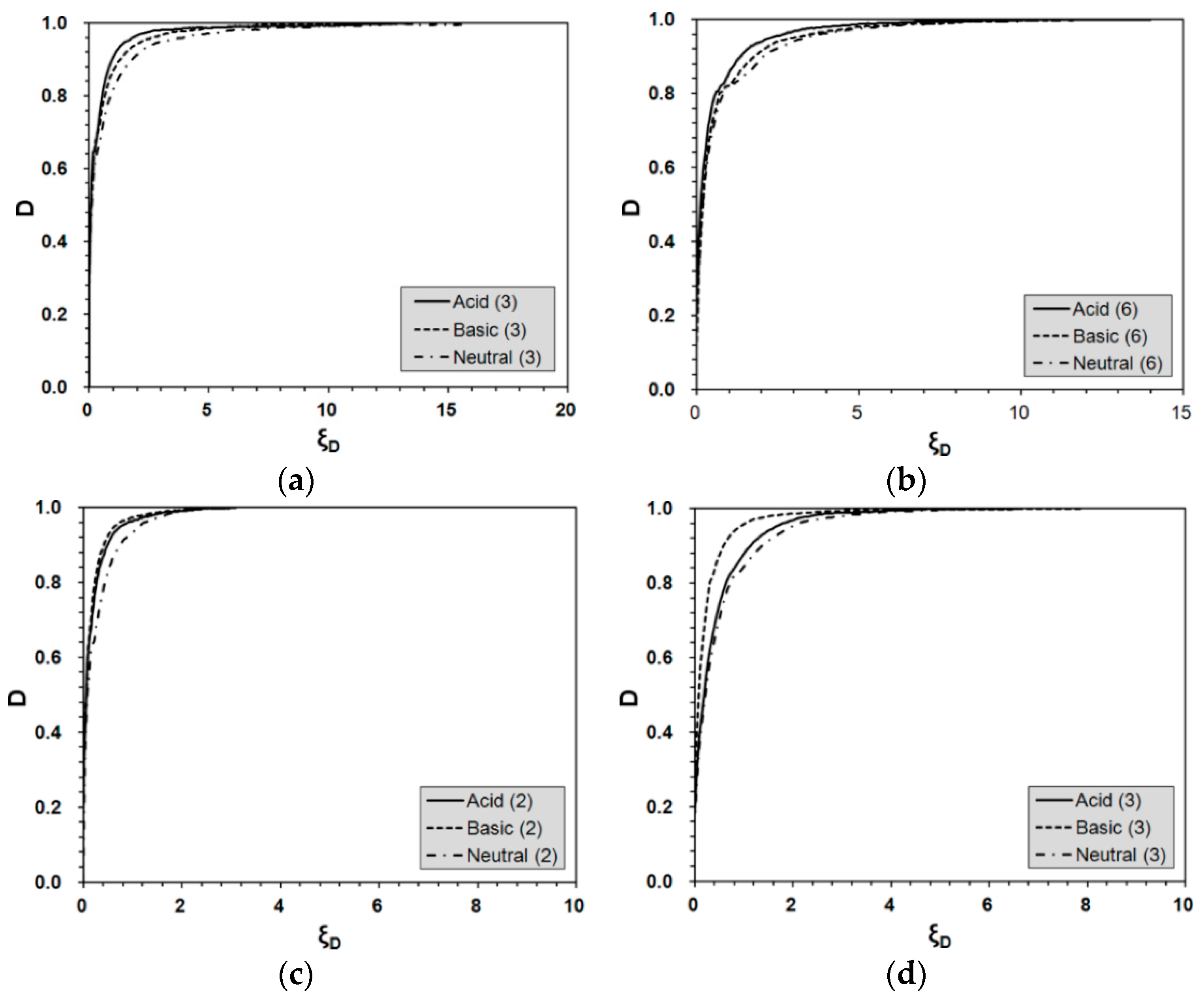
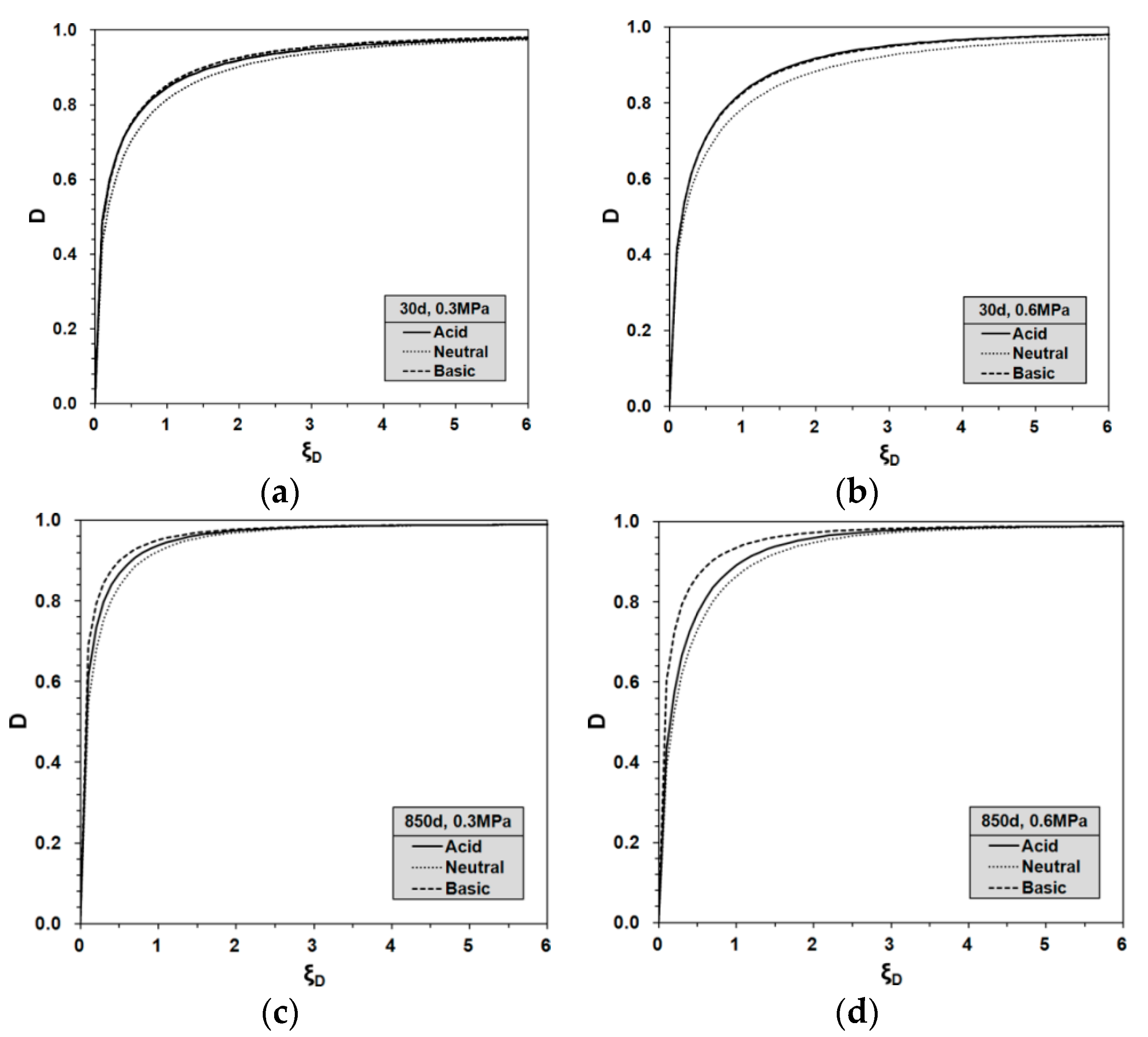
The increase of the disturbance, , represents an increase in the degree of damage in the geosynthetic–soil interface. In the experiment results, the shape of the disturbance function varied in accordance with the chemical conditions. Figure 7 demonstrates the comparison results of the disturbance function curves according to the chemical conditions for different submersion periods and normal stresses. In all of the cases, a more substantial disturbance was observed in the behavior of the sample after long-term submersion (of 850 days). The disturbance at the same deviatoric plastic strain trajectory, , showed larger values under acid conditions in case of short-term submersion, which means that the shear resistance of the geosynthetic–soil interface is more vulnerable to acid conditions in the short term. For behavior after long-term submersion, the disturbance showed larger values under basic conditions, which means that the shear resistance of the geosynthetic–soil interface is more vulnerable to basic conditions in long-term exposure.
The characteristics of the interface–shear behavior can be expressed by the disturbance function curves. Conversely, the disturbance function curve can be reproduced by a mathematical combination of the functional form of the curve and the disturbance parameters and . The parameters represent the intrinsic material characteristics and are determined by a linear regression of the curves from the laboratory test results. The specific procedure and technique are described in a previous study [25]. Table 3 shows the average values of the and parameters based on the test results.
The parameter increased with the increase in the submersion period under the same chemical and normal stress conditions, and is denoted by the shape of the disturbance curve that tends to move left [4]. The geosynthetic–soil interface therefore underwent more damage at low plastic strain levels. Specifically, the interface approached failure despite low plastic strain according to the increase in the submersion period. On the contrary, the parameter decreased with the increase in the normal stress under the same chemical and submersion conditions, which is demonstrated by the tendency of the disturbance curve to move right. Therefore, the geosynthetic–soil interface manifested more resistance against damage at low plastic strain levels. This trend is identical to the characteristics of the shear stress degradation that were analyzed previously. The parameter increased with the increase in the submersion period and the normal stress under the same chemical conditions. This is denoted by the tendency of the curve slope to increase, which also means a rapid increase of the material damage; in particular, the damage significantly grew with small incremental increases in the plastic strain.
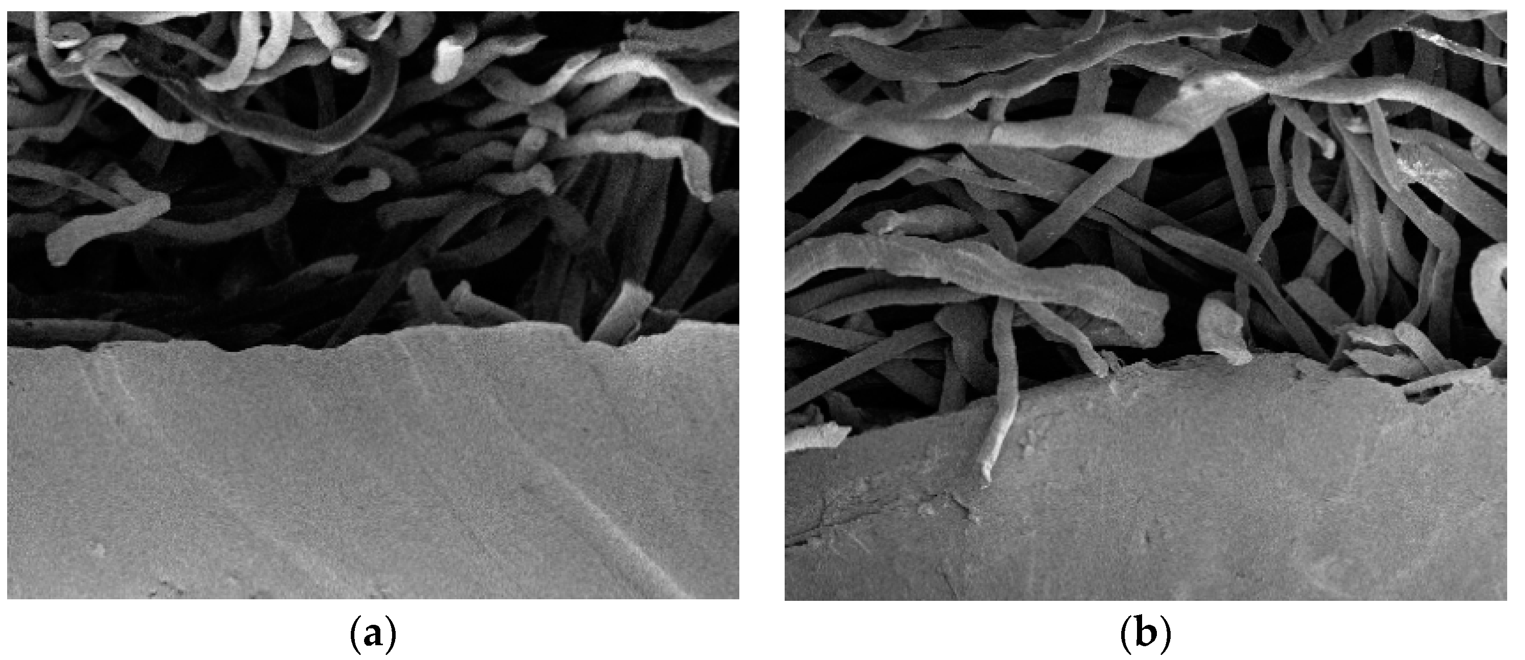
The chemical stability of the HDPE geonet was verified by a few previous papers [36,37], therefore it was deduced that the shear stress degradation of the geosynthetic–soil interface mainly originated due to the different patterns of soil particles. Though the partial decay and breakage of nonwoven fabric filament were found in focused ion beam (FIB) observations, however, the frequency and severity of the observed damage indicate that they might be a minor factor of damage on geosynthetic itself [4]. This hypothesis was successfully verified by the FIB observation. The antioxidant and other ingredients, such as carbon black, showed evident chemical resistance in the HDPE geonet, as shown in Figure 8. On the contrary, severe surface exfoliation of soil particles was widely observed under acidic conditions and pitting on the soil surface was observed under basic conditions. Therefore, it is concluded that the different damage patterns of soil particles mostly entailed the variation of the disturbance function curves and, accordingly, different and parameters were estimated.
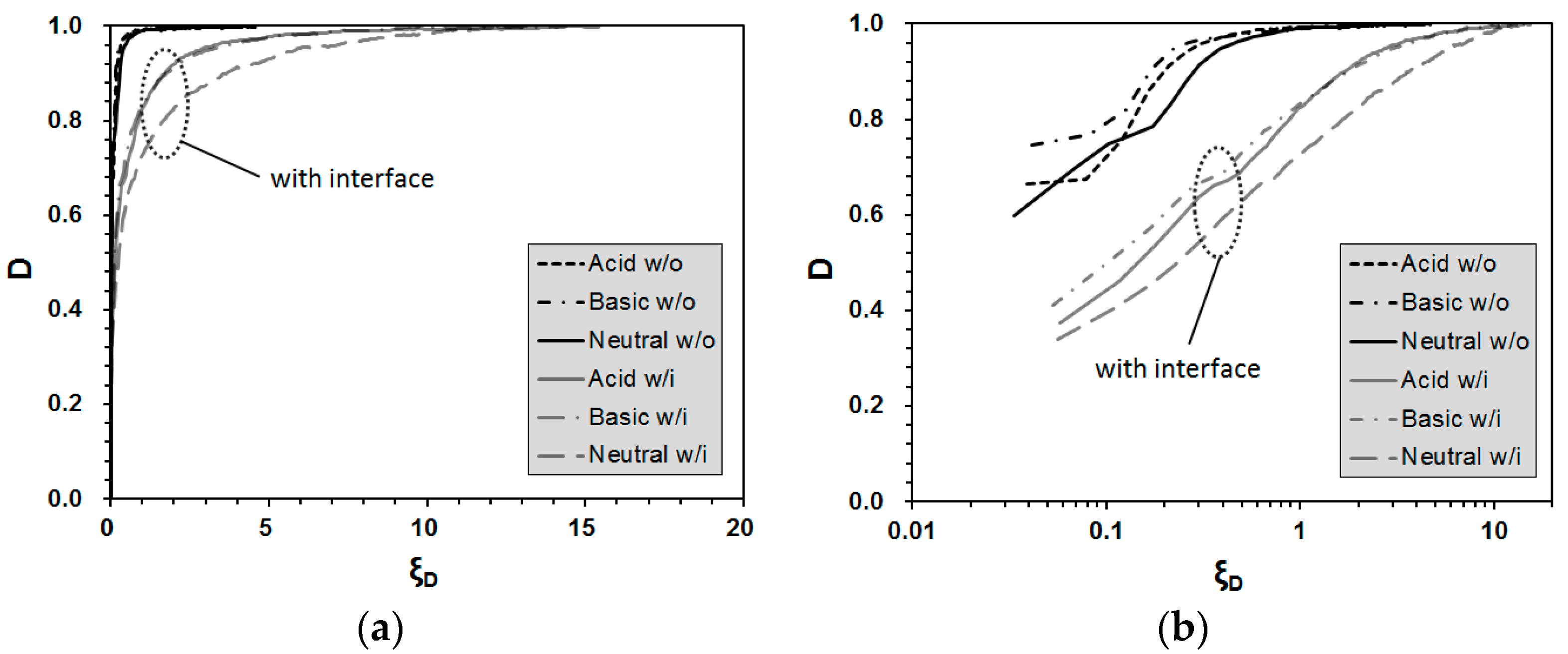
Cyclic simple shear tests on soil alone were performed after prolonged exposure to acidic and basic leachate solutions in order to verify the effect of chemical aggressors on soil. The results were compared with the test results for the geosynthetic–soil interface in Figure 9. Without the interface, basic conditions approached the FA state at the smallest shear strain level, which is the identical trend as the results for the geosynthetic–soil interface. As a result, the disturbance increased more rapidly in the sample without the interface.
Figure 10 displays the new disturbance function curves according to the suggested and parameters. Based on the newly suggested disturbance function curves, the disturbance variation could be obtained quantitatively. Generally, the disturbance intensified after long-term submersion conditions in all of the cases, however, the difference in the disturbance decreased in the cases of higher normal stress conditions, because the confining effect may resist the abrupt progress of the damage in the geosynthetic–soil interface. The variation of the disturbance curve under each submersion period is significant, and the largest variation was observed under the basic conditions for which 0.3 MPa of the normal stress was applied. Figure 11a shows the maximum decrease of the disturbance under a stress of 0.3 MPa, and Table 4 summarizes the maximum decreases of the disturbance for the results for the 30-day and 850-day submersion periods. In Figure 11b, a log scale for strain axis is applied to exhibit the change in disturbance value at low strain level (<2%), therefore, a log scale chart can be useful in the case that the change of disturbance has mainly occurred at low strain levels.
5. Numerical Back-Prediction of Test Results
5.1. Methodology
The numerical back-prediction for the reproduction of the cyclic shear stress–strain relationship was developed according to numerical interpolation procedures. The reproduction of the curves is important in order to significantly reduce the number of laboratory tests, and to predict shear stress degradation of the interface. The methodology of numerical back-prediction is based on the idea that the hysteretic curve at a certain cycle can be divided into 4 phases and each curve can be equally divided into 10 segments again for numerical interpolation. The tangential slopes of the initial and final stress points in a curve can be calculated by linear tangential equations in sequence. Numerical interpolation enables one to obtain the cyclic shear stress–strain values at the midpoints in each segment and to reproduce the cyclic shear stress–strain curves. Shear stress degradation was automatically calculated from the test results and the shear strain increment, and was updated at the target cycle. The RI state was considered as the first cycle, and the FA was considered as the condition after 50th cycle of loading. The procedures for the numerical back-prediction are as follows:
- (1)
- Obtain the DSC parameters and from the experimental test results.
- (2)
- (3)
- Numerical interpolation: Equally divide each phase by “n” segments, and obtain the average tangential gradient by dividing the difference between the initial tangential gradient (GVL) and the final tangential gradient (GEVL), as demonstrated in Figure 13. Then, the linear equations at each dividing point (k/n, 2k/n, …) can be generated, as shown in Figure 13. The total number of the linear equations is (n + 1), and n = 10 was applied in the present study. Therefore, the equation of the initial tangential line can be expressed using Equation (5), and the general equations are expressed using Equations (6)–(8) in the virgin loading phase.
It is assumed that two consecutive linear equations intersect at the midpoint between the two consecutive dividing points. Practically speaking, GVL (the tangential gradient of the starting point of virgin loading) and GBRL (the tangential gradient of the starting point of reloading) are almost identical. In the same manner, the value of GEVL (the tangential gradient of the final point of virgin loading) and GERVL (the tangential gradient of the second final point of reverse loading) and the value of GERL (the tangential gradient of the final point of reloading) and GRVL1,2 (tangential gradient of the point shear strain intercept) are also regarded as the same.
- (4)
- Obtain by combining the yields of Equations (3), (4) and (9). The updated shear stress at each cycle can be obtained using Equation (6).
- (5)
- Obtain the average strain increment: Based on the variation of the shear strain between the RI and FA conditions, the average plastic strain incremental can be calculated. In the present study, the number of cycles that begin to approach the FA state is considered as 50.
- (6)
- Update : Based on the result of Equation (9) and the average strain increment from the procedure of Equation (7), the cyclic shear stress at any cycle can be calculated.
5.2. Back-Prediction Results
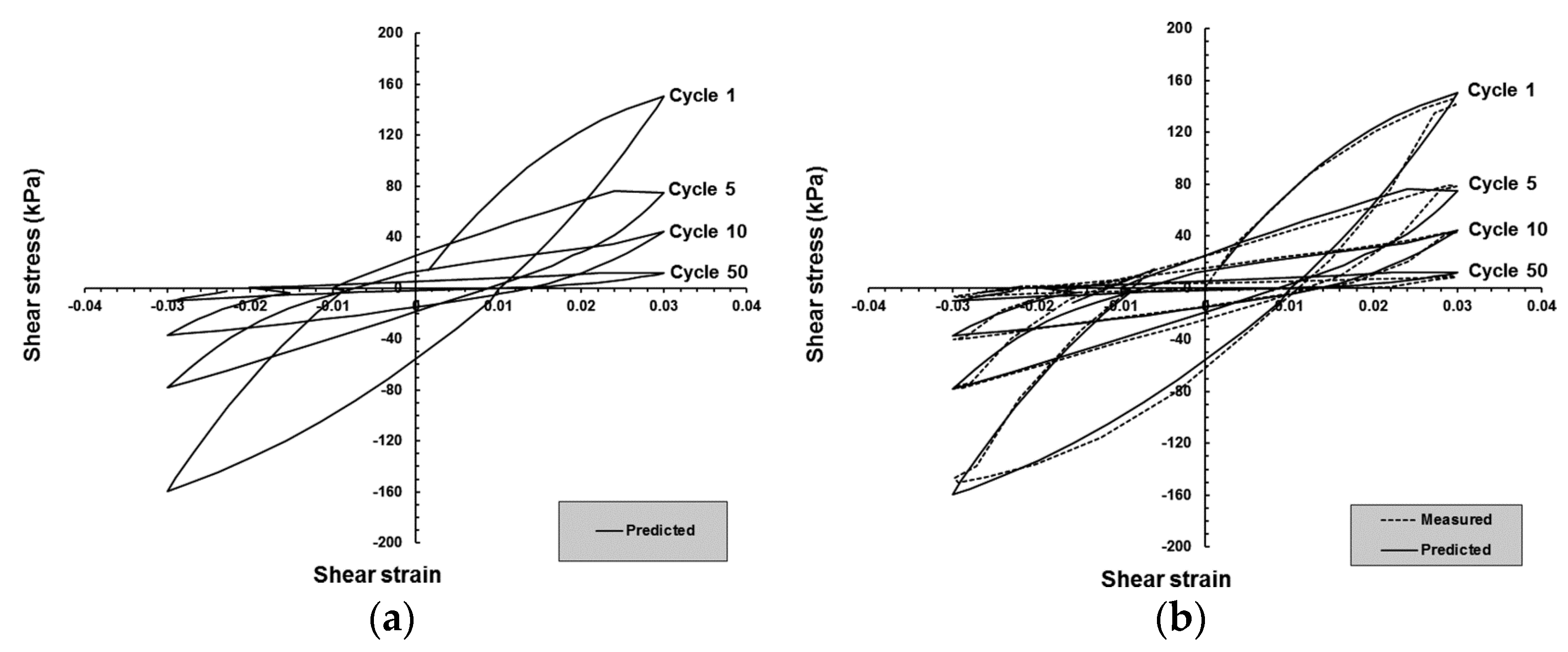
Once the cyclic shear stresses from the RI () and FA () states are obtained with the strain, the cyclic shear degradation behavior can be simulated based on the disturbance function parameters. A summary of the developed model parameters of the present study is already shown in Table 3. Figure 14a displays the reproduced stress–strain curves based on the developed numerical interpolation, while Figure 14b demonstrates the comparison between the measured and predicted results for the acidic conditions. The cyclic shear stress–strain curves were obtained at the 1st, 5th, 10th, and 50th cycles. Table 5 shows the comparison of the measured and predicted gradients for the 1st cycle according to the proposed method.
As shown in Figure 14, although a few discrepant points were observed, the comparison results demonstrated sound agreement in general. A few discrepancies occurred at the shear strain, and these correspond to the asymmetric stress response of the soil specimen that was due to its anisotropy, inhomogeneity, and the reorientation of the particles from the stress reversal under the cyclic loading [38]. Soil is not a homogeneous and isotropic material itself because it is composed of erratic shaped minerals, complex combinations of pore water, etc. It causes irregular and biased behavior. Therefore, this kind of error is unavoidable in a numerical simulation of the response under cyclic loading. However, the cyclic shear stress degradation is generally in good agreement.
Apart from the comparison results in Figure 14, it is important to verify that the predicted DSC parameters which are not obtained from the test results directly can simulate the shear stress–strain behavior. To compare the predicted shear stress–strain results with the experimental results, additional cyclic simple shear tests were conducted in accordance with new conditions that are displayed in Table 6.
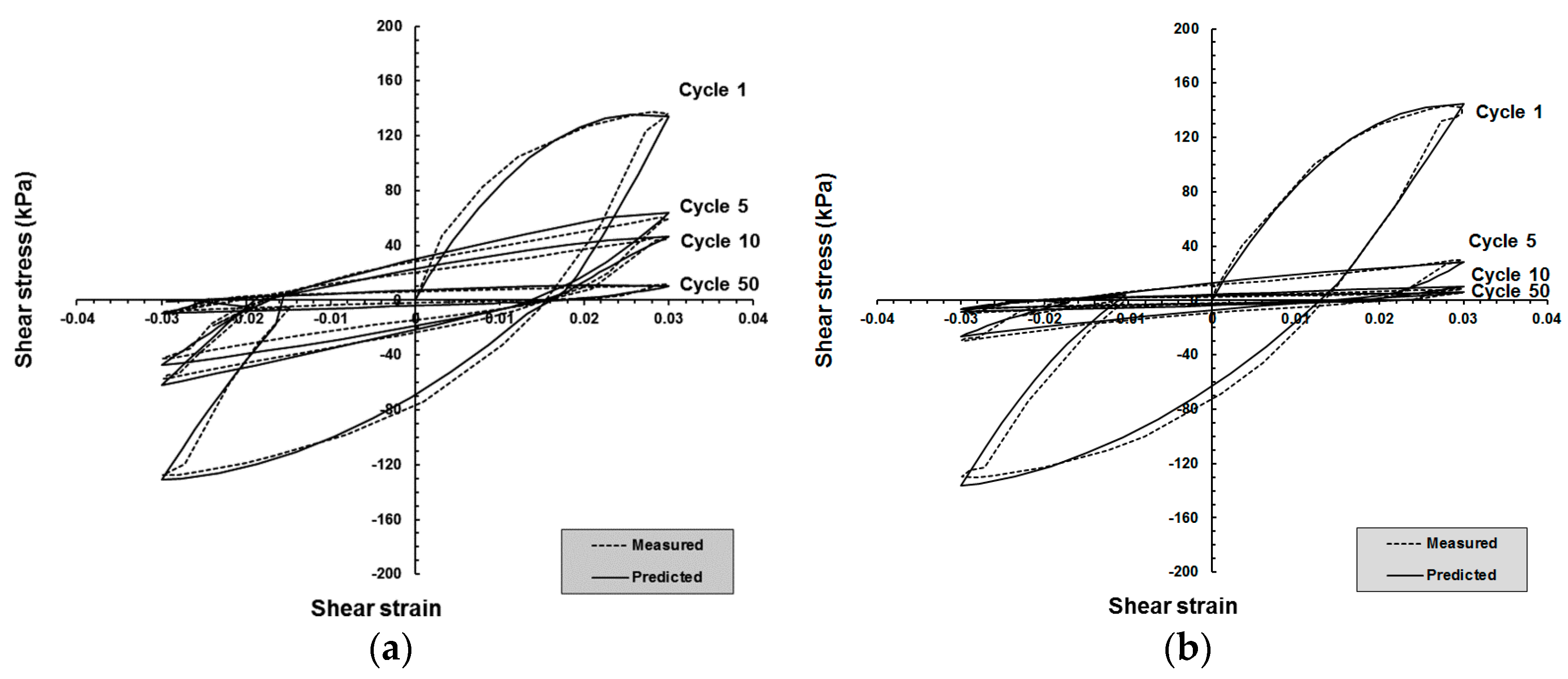
The submersion period was approximately 12 months, and the DSC parameters for 0.45 MPa of normal stress were predicted using the suggested linear interpolation in the present study. Based on the proposed methodology, the shear stress–strain response was predicted and compared with the test results at the 1st, 5th, 10th, and 50th cycles, as shown in Figure 15. The predicted result can simulate the shear stress–strain curves and the shear stress degradation according to the loading cycles, and the comparison results displayed sound agreement.
The numerical back-prediction of the geosynthetic–soil interface was derived in consideration of the chemical effects that are expected to be the basis of the future construction of a fully numerical analysis for which universal codes will be used. At that point, a large number of laboratory tests could be reduced.
6. Conclusions
The shear behaviors of waste landfill systems under dynamic (earthquake) loading are significantly influenced by the response of the interfaces that are composed of geosynthetics and soil. A few conclusions were obtained from the present study, as follows:
- (1)
- The new disturbance function parameters, and , were estimated using a linear regression technique. Parameter increased with the increase of the submersion period under the same chemical and normal stress conditions. On the contrary, parameter decreased with the increase of the normal stress under the same chemical and submersion conditions. Parameter increased with the increase of the submersion period and the normal stress under the same chemical conditions.
- (2)
- Based on the test results and the new disturbance function parameters, the new disturbance function curves that correspond to the chemical conditions were evaluated. For the short-term submersion (30 days), the acid condition causes more vulnerability. For the long-term submersion, the difference in the disturbance function value at a certain deviatoric plastic strain trajectory, , was more distinct than that of the value after short-term submersion. In all of cases, acidic conditions caused the most vulnerability for the geosynthetic–soil interface for short-term submersion, and the basic conditions caused the most vulnerable for long-term submersion.
- (3)
- The variation between the disturbance curves for each submersion period was significant, and the largest variation was under the basic conditions in which 0.3 MPa of normal stress was applied. The variation between the disturbance curves under each normal stress condition was also remarkable, and the largest variation was for the acidic conditions for the 850-day submersion period.
- (4)
- The performance of the numerical back-prediction of the cyclic shear stress–strain relationship is based on the numerical interpolation procedures that are suggested in the present study. Based on the experiment data, the DSC parameters were utilized to reproduce the cyclic shear stress according to the loading cycle. The back-prediction result was also verified by a comparison between the predicted data and the measured data, and sound agreements were demonstrated. Furthermore, the compatibility and accuracy of the DSC parameters, and were ensured.
- (5)
- The proposed methodology can be used in seismic design procedures of a waste landfill. First of all, only a few seismic simple shear tests need to be performed for representative disturbance functions and parameters to be obtained. Then, those parameters can be verified by numerical back-prediction in order to reduce a large number of laboratory tests. If a considerable number of laboratory tests are performed, the guideline of critical shear strain under dynamic conditions shall be suggested in a further study.
- (6)
- In the future, it is expected that the numerical back-prediction of the geosynthetic–soil interface will serve as the basis of a fully numerical analysis. The numerical back-prediction is capable of considering the shear stress degradation with a sufficient accuracy to reducing a large number of laboratory tests. Based on the representative parameters which are verified by numerical back-prediction, the estimated shear strain can be used as a criterion under seismic conditions. Test are performed with limited number of factors (such as normal stress, material, chemical aggressors, etc.), therefore, it is still difficult to suggest typical back-bone curves. Relevant research will be performed in a further study.
Acknowledgments
The present paper was developed in 2014 by Hanseo University as an in-school research support project.
Author Contributions
Changwon Kwak and Innjoon Park conceived of the theme, and idea, and organized the framework. Junboum Park checked numerical back-prediction. Dongin Jang performed the M-PIA tests required for the paper; and Changwon Kwakand Innjoon Park wrote the paper.
Conflicts of Interest
The authors declare no conflict of interest.
References
- Orloff, K.; Falk, H. An international perspective on hazardous waste practices. Int. J. Hyg. Environ. Health 2003, 206, 291–302. [Google Scholar] [CrossRef] [PubMed]
- Mor, S.; Ravindra, K.; Dahiya, R.P.; Chandra, A. Leachate characterization and assessment of groundwater pollution near municipal solid waste landfill site. Environ. Monit. Assess. 2006, 118, 435–456. [Google Scholar] [CrossRef] [PubMed]
- Bouazza, A.; Zornberg, J.G.; Adam, D. Geosynthetics in waste containment facilities: Recent advances. In Proceedings of the 7th International Conference on Geosynthetics, Nice, France, 22–27 September 2007; Volume 90, pp. 445–507. [Google Scholar]
- Kwak, C.W. Cyclic Shear Behaviors of Geosynthetic-Soil Interface Considering Chemical Effects. Ph.D. Thesis, Department of Civil and Environmental Engineering, Seoul National University, Seoul, Korea, 2014. [Google Scholar]
- Stark, T.D.; Williamson, T.A.; Eid, H.T. HDPE geomembrane/geotextile interface shear strength. J. Geotech. Eng. 1996, 122, 197–203. [Google Scholar] [CrossRef]
- Nguyen, Q.V.; Fatahi, B.; Hokmabadi, A.S. Influence of Size and Load-Bearing Mechanism of Piles on Seismic Performance of Buildings Considering Soil-Pile-Structure Interaction. Int. J. Geomech. 2017, 17, 04017007. [Google Scholar] [CrossRef]
- Seo, M.W.; Park, I.J.; Park, J.B. Development of displacement-softening model for interface shear behavior between geosynthetics. Soils Found. 2004, 44, 27–38. [Google Scholar] [CrossRef]
- Seo, M.W.; Park, J.B.; Park, I.J. Evaluation of interface shear strength between geosynthetics under wet condition. Soils Found. 2007, 47, 845–856. [Google Scholar] [CrossRef]
- De, A.; Zimmie, T.F. Landfill Stability: Static and Dynamic Geosynthetic Interface Friction Value; Geosynthetic Asia’97; Brookfield: Bangalore, India, 1997; pp. 271–278. [Google Scholar]
- Fishman, K.L.; Pal, S. Further study of geomembrane/cohesive soil interface shear behavior. Geotext. Geomembr. 1994, 13, 571–590. [Google Scholar] [CrossRef]
- Ghosh, B.; Fatahi, B.; Khabbaz, H.; Yin, J.H. Analytical study for double-layer geosynthetic reinforced load transfer platform on column improved soft soil. Geotext. Geomembr. 2017, 45, 508–536. [Google Scholar] [CrossRef]
- Ghosh, B.; Fatahi, B.; Khabbaz, H. Analytical Solution to Analyze LTP on Column-Improved Soft Soil Considering Soil Nonlinearity. Int. J. Geomech. 2017, 17, 04016082-1–04016082-24. [Google Scholar] [CrossRef]
- Hokmabadi, A.S.; Fatahi, B. Influence of Foundation Type on Seismic Performance of Buildings Considering Soil-Structure Interaction. Int. J. Struct. Stab. Dyn. 2016, 16, 1550043. [Google Scholar] [CrossRef]
- Armaleh, S.H.; Desai, C.S. Modeling Include Testing of Cohesionless Soils under Disturbed State Concept; Department of Civil Engineering and Engineering Mechanics, University of Arizona: Tuscon, AZ, USA, 1990. [Google Scholar]
- Ma, Y. Disturbed State Concept for Rock Joints; Department of Civil Engineering and Engineering Mechanics, University of Arizona: Tuscon, AZ, USA, 1990. [Google Scholar]
- Rigby, D.B.; Desai, C.S. Testing, Modeling, and Application of Saturated Interfaces in Dynamic Soil-Structure Interaction; Department of Civil Engineering and Engineering Mechanics, University of Arizona: Tuscon, AZ, USA, 1995. [Google Scholar]
- Park, I.J.; Yoo, J.H.; Kim, S.I. Disturbed state modeling for dynamic analysis of soil-structure interface. J. KGS 2000, 16, 5–13. [Google Scholar]
- Kjeldsen, P.; Barlaz, M.A.; Rooker, A.P.; Baun, A.; Ledin, A.; Christensen, T.H. Present and long-term composition of MSW landfill leachate: A review. Crit. Rev. Environ. Sci. Technol. 2002, 32, 297–336. [Google Scholar] [CrossRef]
- Oweis, I.S.; Khera, R.P. Geotechnology of Waste Management, 2nd ed.; PWS Publishing Company: Boston, MA, USA, 1998; pp. 1–24 & 295–299. [Google Scholar]
- Bilgili, M.S.; Demir, A.; Ince, M.; Ozkaya, B. Metal concentrations of simulated aerobic and anaerobic pilot scale landfill reactors. J. Hazard. Mater. 2007, 145, 186–194. [Google Scholar] [CrossRef] [PubMed]
- Kwak, C.W.; Park, I.J.; Park, J.B. Evaluation of disturbance function for geosynthetic–soil interface considering chemical reactions based on cyclic direct shear tests. Soils Found. 2013, 53, 720–734. [Google Scholar] [CrossRef]
- Rafizul, I.M.; Alamgir, M. Characterization and tropical seasonal variation of leachate: Results from landfill lysimeter studied. Waste Manag. 2012, 32, 2080–2095. [Google Scholar] [CrossRef] [PubMed]
- Desai, C.S. A consistent finite element technique for work-softening behavior. In Proceedings of the International Conference on Computer Mechanics in Nonlinear Mechanics; University of Texas Press: Austin, TX, USA, 1974. [Google Scholar]
- Desai, C.S.; Ma, Y. Modeling of joints and interfaces using the disturbed state concept. Int. J. Numer. Anal. Methods Geomech. 1992, 16, 623–653. [Google Scholar] [CrossRef]
- Kwak, C.W.; Park, I.J.; Park, J.B. Modified cyclic shear test for evaluating disturbance function and numerical formulation of geosynthetic-soil interface considering chemical effect. Geotech. Test. J. 2013, 36, 553–567. [Google Scholar] [CrossRef]
- Park, I.J. Disturbed State Modeling for Dynamic and Liquefaction Analysis; Department of Civil Engineering and Engineering Mechanics, University of Arizona: Tuscon, AZ, USA, 1997. [Google Scholar]
- Kwak, C.W.; Park, I.J.; Park, J.B. Development of Modified Interface apparatus and prototype cyclic simple shear test considering chemical and thermal effects. Geotech. Test. J. 2016, 39, 20–34. [Google Scholar] [CrossRef]
- ASTM D5035-11. Standard Test Method for Breaking Force and Elongation of Textile Fabrics (Strip Method); ASTM International: West Conshohocken, PA, USA, 2015. [Google Scholar]
- Ling, H.I.; Wang, J.P.; Leshchinsky, D. Cyclic behavior of soil-structure interfaces associated with modular-block reinforced soil-retaining walls. Geosynth. Int. 2008, 15, 14–21. [Google Scholar] [CrossRef]
- Masada, T.; Mithell, G.F.; Sargand, S.M.; Shashikumar, B. Modified direct shear study of clay liner-geomembrane interfaces exposed to landfill leachate. Geotext. Geomembr. 1994, 13, 165–179. [Google Scholar] [CrossRef]
- Stessel, R.I.; Hodge, J.S. Chemical resistance testing of geomembrane liners. J. Hazard. Mater. 1995, 42, 265–287. [Google Scholar] [CrossRef]
- Ehrig, H.J. Water and element balances of landfills. In The Landfill; Baccini, P., Ed.; Springer: Berlin, Germany, 1988; pp. 83–115. [Google Scholar]
- Shibuya, S.; Mitachi, T.; Fukuda, F.; Degoshi, T. Strain-rate effects on shear modulus and damping of normally consolidated clay. Geotech. Test. J. 1995, 18, 365–375. [Google Scholar]
- Araei, A.A.; Razeghi, H.R.; Tabatabaei, S.H.; Ghalandarzadeh, A.; Tabatabaei, S.H. Effects of loading rate and initial stress state on stress-strain behavior of rock fill materials under monotonic and cyclic loading conditions. Sci. Iran. A 2012, 19, 1220–1235. [Google Scholar] [CrossRef]
- ASTM D3999. Standard Test Methods for the Determination of the Modulus and Damping Properties of Soils Using the Cyclic Triaxial Apparatus; ASTM International: West Conshohocken, PA, USA, 1996. [Google Scholar]
- Koerner, R.M. Designing with Geosynthetics, 6th ed.; Xlibris Corporation: Lexington, KY, USA, 2013; Volume 1, pp. 165–173. [Google Scholar]
- Rowe, R.K.; Sangam, H.P. Durability of HDPE Geomembranes. Geotext. Geomembr. 2002, 20, 77–95. [Google Scholar] [CrossRef]
- Thurairajah, A. Shear behavior of sand under stress reversal. In Proceedings of the 8th International Conference on Soil Mechanics and Foundation Engineering, Moscow, Russia, 6–11 August 1973; Volume 1, pp. 439–445. [Google Scholar]
Figure 1.
Section of waste landfill and concept of geosynthetic–soil interface [4].
Figure 1.
Section of waste landfill and concept of geosynthetic–soil interface [4].
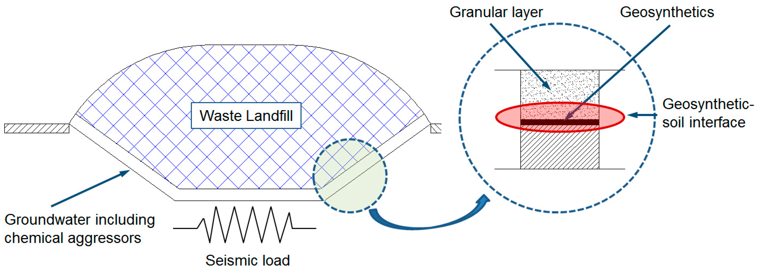
Figure 2.
Shear stress of RI, FA, and observed states.

Figure 3.
M-PIA: (a) photo and (b) shear-box details.
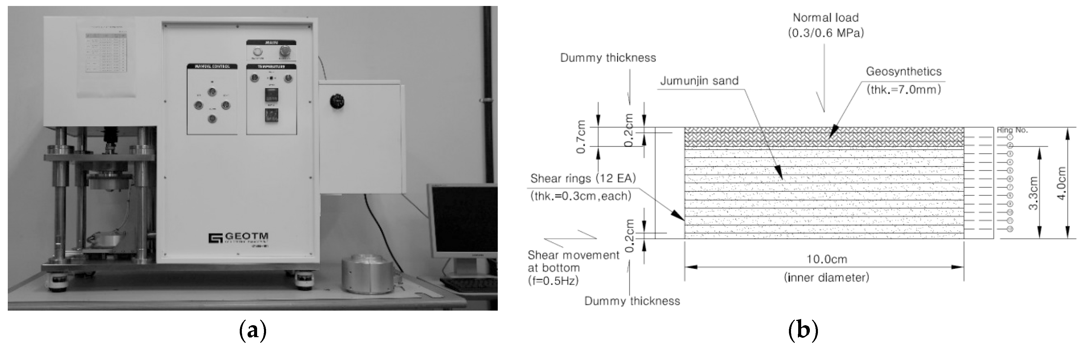
Figure 4.
Test schedule.

Figure 5.
Typical shear stress–strain curves for the 30-day submersion period: (a,c,e) = 0.3 MPa of normal stress; and (b,d,f) = 0.6 MPa of normal stress.
Figure 5.
Typical shear stress–strain curves for the 30-day submersion period: (a,c,e) = 0.3 MPa of normal stress; and (b,d,f) = 0.6 MPa of normal stress.


Figure 6.
Typical shear stress–strain curves for the 850-day submersion period: (a,c,e) = 0.3 MPa of normal stress; and (b,d,f) = 0.6 MPa of normal stress.
Figure 6.
Typical shear stress–strain curves for the 850-day submersion period: (a,c,e) = 0.3 MPa of normal stress; and (b,d,f) = 0.6 MPa of normal stress.

Figure 7.
Typical disturbance function curves: (a) 30 days submersion, 0.3 MPa of normal stress; (b) 30 days submersion, 0.6 MPa of normal stress; (c) 850 days submersion, 0.3 MPa of normal stress; (d) 850 days submersion, 0.6 MPa of normal stress.
Figure 7.
Typical disturbance function curves: (a) 30 days submersion, 0.3 MPa of normal stress; (b) 30 days submersion, 0.6 MPa of normal stress; (c) 850 days submersion, 0.3 MPa of normal stress; (d) 850 days submersion, 0.6 MPa of normal stress.

Figure 8.
Microscopic observation results (100×): (a) 850 days submersion, acidic; (b) 850 days submersion, basic.
Figure 8.
Microscopic observation results (100×): (a) 850 days submersion, acidic; (b) 850 days submersion, basic.

Figure 9.
Disturbance function curves for soil alone versus with interface after 850 days submersion, 0.3 MPa: (a) natural scale; (b) log scale.
Figure 9.
Disturbance function curves for soil alone versus with interface after 850 days submersion, 0.3 MPa: (a) natural scale; (b) log scale.

Figure 10.
New disturbance function curves: (a) 30 days submersion, 0.3 MPa; (b) 30 days submersion, 0.6 MPa; (c) 850 days submersion, 0.3 MPa; and (d) 850 days submersion, 0.6 MPa.
Figure 10.
New disturbance function curves: (a) 30 days submersion, 0.3 MPa; (b) 30 days submersion, 0.6 MPa; (c) 850 days submersion, 0.3 MPa; and (d) 850 days submersion, 0.6 MPa.

Figure 11.
Maximum decreases of the disturbance (ΔDmax) under 0.3 MPa: (a) natural scale for strain axis; (b) log scale for strain axis.
Figure 11.
Maximum decreases of the disturbance (ΔDmax) under 0.3 MPa: (a) natural scale for strain axis; (b) log scale for strain axis.
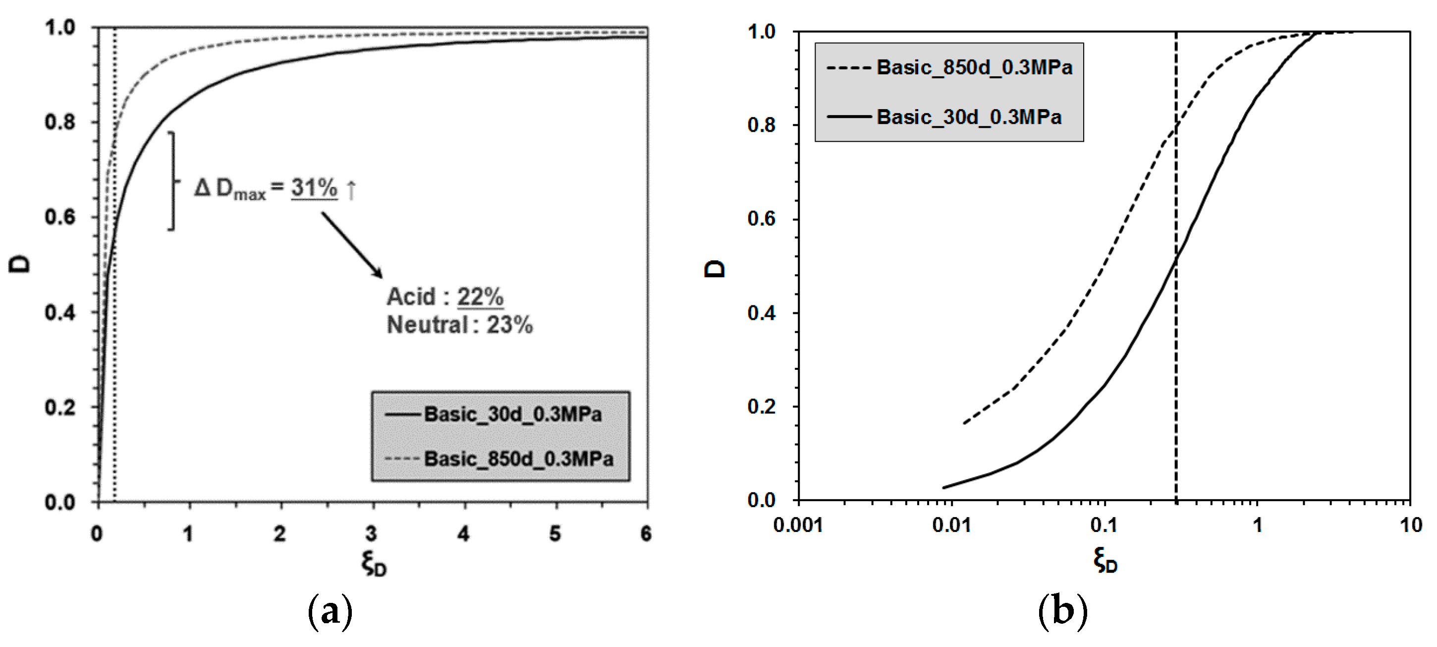
Figure 12.
Definition of each phase in a curve: (a) four phases in a cyclic loading and (b) tangential gradients to define each phase [4].
Figure 12.
Definition of each phase in a curve: (a) four phases in a cyclic loading and (b) tangential gradients to define each phase [4].
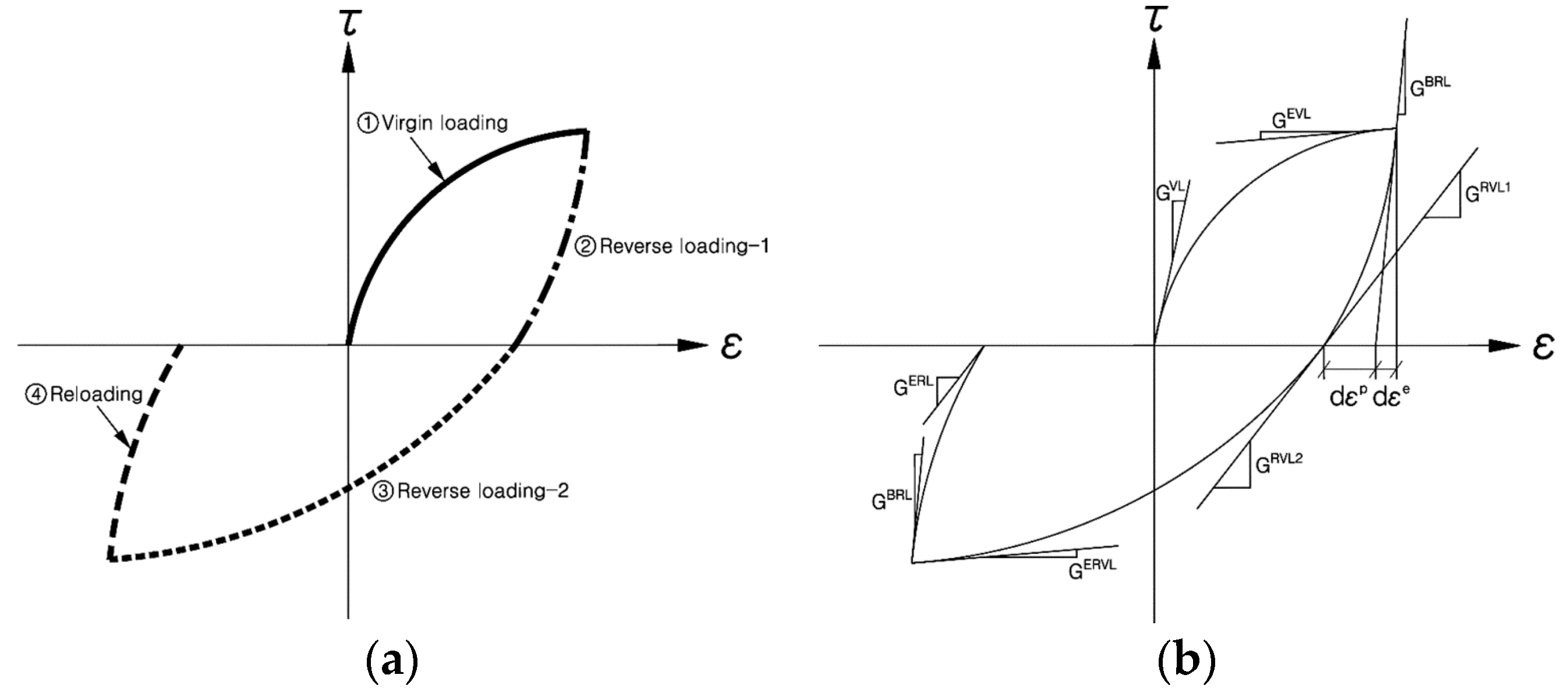
Figure 13.
Numerical interpolation of a cyclic loop [16].
Figure 13.
Numerical interpolation of a cyclic loop [16].
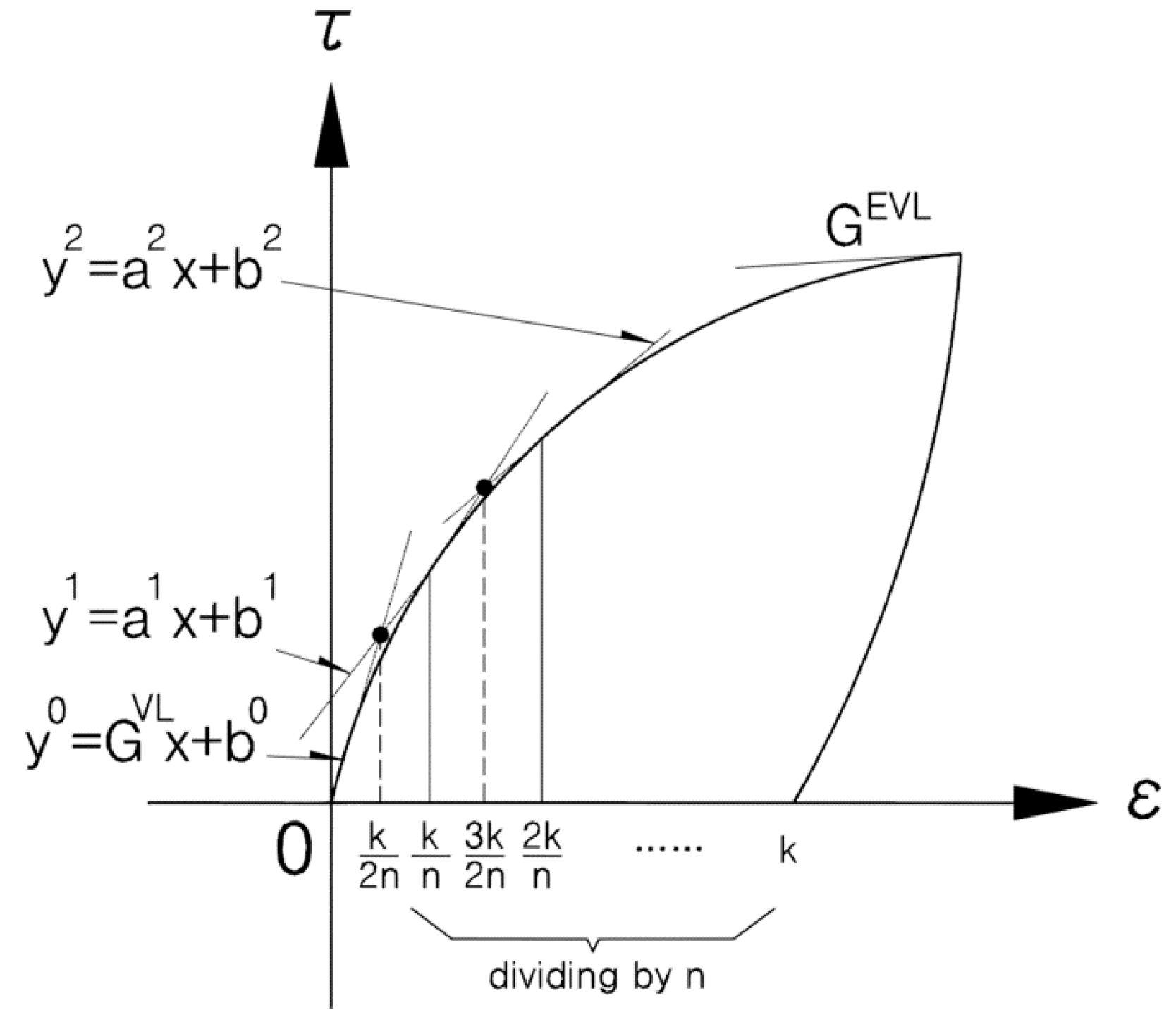
Figure 14.
Numerical interpolation results: (a) predicted; (b) comparison between measured and predicted results.
Figure 14.
Numerical interpolation results: (a) predicted; (b) comparison between measured and predicted results.

Figure 15.
Verification of the predicted results (360 days submersion, 0.45 MPa): (a) basic; (b) acid.
Figure 15.
Verification of the predicted results (360 days submersion, 0.45 MPa): (a) basic; (b) acid.


Table 1.
Physical properties of Jumunjin sand.
| Gs | Max. Dry Density (kN/m3) | Min. Dry Density (kN/m3) | Max. Void Ratio | Min. Void Ratio | Relative Density (%) | Moist Content (%) |
|---|---|---|---|---|---|---|
| 2.63 | 16.70 | 13.85 | 0.915 | 0.535 | 60 | 33.0 |
Table 2.
Specifications of the geocomposite.
| Type | Geocomposite (Geonet + Nonwoven Fabric) |
|---|---|
| Manufacturer | GOLDENPOW, Korea |
| Ingredients | Geonet (High Density Polyethylene, HDPE), nonwoven fabric (Polyethylene Terephthalate(PET) + polypropylene (PP)), Carbon black (antioxidant; 2.2%) |
| Thickness | 7.0 mm |
| Tensile strength (kN/m) | 18.1 (longitudinal)/7.6 (transversal) |
| Unit weight (kN/m3) | 4.62 |
| Density (kN/m3) | 9.29 |
| Tensile strength (N/cm) | 141.4 (ASTM D5035-11 [28]) |
Table 3.
and parameters.
| Submersion Period (Days) | Normal Stress (MPa) | Chemical Condition | Parameters | Avg. |
|---|---|---|---|---|
| 30 | 0.3 | Acid | 1.9269 | |
| 0.4536 | ||||
| Neutral | 1.7287 | |||
| 0.4859 | ||||
| Basic | 1.9723 | |||
| 0.4768 | ||||
| 0.6 | Acid | 1.8193 | ||
| 0.5260 | ||||
| Neutral | 1.5810 | |||
| 0.4972 | ||||
| Basic | 1.7989 | |||
| 0.5179 | ||||
| 850 | 0.3 | Acid | 2.9476 | |
| 0.4852 | ||||
| Neutral | 2.7061 | |||
| 0.5286 | ||||
| Basic | 3.2338 | |||
| 0.4329 | ||||
| 0.6 | Acid | 2.3057 | ||
| 0.6040 | ||||
| Neutral | 2.0655 | |||
| 0.6179 | ||||
| Basic | 2.9057 | |||
| 0.4885 |
Table 4.
Maximum variations of the disturbance curves.
| Chemical Conditions | Max. Decreases of Disturbance (Δ Dmax) (between the Results of 30 and 850 Days of Submersion) | ||
|---|---|---|---|
| Basic | Neutral | Acid | |
| 0.3 MPa of normal stress | 31 % | 23 % | 22 % |
| 0.6 MPa of normal stress | 26 % | 10 % | 8 % |
Table 5.
Gradient for back-prediction.
| Cycle | Index | Gradient | |
|---|---|---|---|
| Measured | Predicted | ||
| 1 | GVL | 9184.71 | 8882.43 |
| GEVL | 2120.37 | 1668.50 | |
| GBRL | 9560.71 | 9280.93 | |
| GRVL1 | 5778.57 | 5653.48 | |
| GRVL2 | 5778.57 | 5254.98 | |
| GERVL | 1216.63 | 2465.50 | |
| GBRL | 10,306.53 | 9280.93 | |
| GERL | 5403.29 | 5653.48 | |
Table 6.
Additional test conditions for verification.
| Chemical Conditions | DSC Parameters | Normal Stress (MPa) | ||
|---|---|---|---|---|
| 0.30 | 0.45 (New) | 0.60 | ||
| Basic | 1.5529 | 1.7171 (predicted) | 1.8814 | |
| 0.5287 | 0.5804 (predicted) | 0.6320 | ||
| Acid | 3.3713 | 3.4440 (predicted) | 3.5166 | |
| 0.5175 | 0.6231 (predicted) | 0.7287 | ||
© 2017 by the authors. Licensee MDPI, Basel, Switzerland. This article is an open access article distributed under the terms and conditions of the Creative Commons Attribution (CC BY) license (http://creativecommons.org/licenses/by/4.0/).
Share and Cite
MDPI and ACS Style
Kwak, C.; Park, J.; Jang, D.; Park, I. Dynamic Shear Degradation of Geosynthetic–Soil Interface in Waste Landfill Sites. Appl. Sci. 2017, 7, 1225. https://doi.org/10.3390/app7121225
AMA Style
Kwak C, Park J, Jang D, Park I. Dynamic Shear Degradation of Geosynthetic–Soil Interface in Waste Landfill Sites. Applied Sciences. 2017; 7(12):1225. https://doi.org/10.3390/app7121225
Chicago/Turabian StyleKwak, Changwon, Junboum Park, Dongin Jang, and Innjoon Park. 2017. "Dynamic Shear Degradation of Geosynthetic–Soil Interface in Waste Landfill Sites" Applied Sciences 7, no. 12: 1225. https://doi.org/10.3390/app7121225
Note that from the first issue of 2016, this journal uses article numbers instead of page numbers. See further details here.