
Audio Time Stretching Using Fuzzy Classification of Spectral Bins


Acoustics Laboratory, Department of Signal Processing and Acoustics, Aalto University, FI-02150 Espoo, Finland
*
Author to whom correspondence should be addressed.
Appl. Sci. 2017, 7(12), 1293; https://doi.org/10.3390/app7121293
Submission received: 3 November 2017
/
Revised: 3 December 2017
/
Accepted: 7 December 2017
/
Published: 12 December 2017
(This article belongs to the Special Issue Sound and Music Computing)
Abstract
:A novel method for audio time stretching has been developed. In time stretching, the audio signal’s duration is expanded, whereas its frequency content remains unchanged. The proposed time stretching method employs the new concept of fuzzy classification of time-frequency points, or bins, in the spectrogram of the signal. Each time-frequency bin is assigned, using a continuous membership function, to three signal classes: tonalness, noisiness, and transientness. The method does not require the signal to be explicitly decomposed into different components, but instead, the computing of phase propagation, which is required for time stretching, is handled differently in each time-frequency point according to the fuzzy membership values. The new method is compared with three previous time-stretching methods by means of a listening test. The test results show that the proposed method yields slightly better sound quality for large stretching factors as compared to a state-of-the-art algorithm, and practically the same quality as a commercial algorithm. The sound quality of all tested methods is dependent on the audio signal type. According to this study, the proposed method performs well on music signals consisting of mixed tonal, noisy, and transient components, such as singing, techno music, and a jazz recording containing vocals. It performs less well on music containing only noisy and transient sounds, such as a drum solo. The proposed method is applicable to the high-quality time stretching of a wide variety of music signals.
1. Introduction
Time-scale modification (TSM) refers to an audio processing technique, which changes the duration of a signal without changing the frequencies contained in that signal [1,2,3]. For example, it is possible to reduce the speed of a speech signal so that it sounds as if the person is speaking more slowly, since the fundamental frequency and the spectral envelope are preserved. Time stretching corresponds to the extension of the signal, but this term is used as a synonym for TSM. Audio time stretching has numerous applications, such as fast browsing of speech recordings [4], music production [5], foreign language and music learning [6], fitting of a piece of music to a prescribed time slot [7], and slowing down the soundtrack for slow-motion video [8]. Additionally, TSM is often used as a processing step in pitch shifting, which aims at changing the frequencies in the signal without changing its duration [2,3,7,9,10].
Audio signals can be considered to consist of sinusoidal, noise, and transient components [11,12,13,14]. The main challenge in TSM is in simultaneously preserving the subjective quality of these distinct components. Standard time-domain TSM methods, such as the synchronized overlap-add (SOLA) [15], the waveform-similarity overlap-add [16], and the pitch-synchronous overlap-add [17] techniques, are considered to provide high-quality TSM for quasi-harmonic signals. When these methods are applied to polyphonic signals, however, only the most dominant periodic pattern of the input waveform is preserved, while other periodic components suffer from phase jump artifacts at the synthesis frame boundaries. Furthermore, overlap-add techniques are prone to transient skipping or duplication when the signal is contracted or extended, respectively. To solve this, transients can be detected and the time-scale factor can be changed during transients [18,19].
Standard phase vocoder TSM techniques [20,21] are based on a sinusoidal model of the input signal. Thus, they are most suitable for processing of signals which can be represented as a sum of slowly varying sinusoids. Even with these kind of signals however, the phase vocoder TSM introduces an artifact typically described as “phasiness” to the processed sound [21,22]. Furthermore, transients processed with the standard phase vocoder suffer from a softening of the perceived attack, often referred to as “transient smearing” [2,3,23]. A standard solution for reducing transient smearing is to apply a phase reset or phase locking at detected transient locations of the input signal [23,24,25].
As another approach to overcome these problems in the phase vocoder, TSM techniques using classification of spectral components based on their signal type have been proposed recently. In [26], spectral peaks are classified into sinusoids, noise, and transients, using the methods of [23,27]. Using the information from the peak classification, the phase modification applied in the technique is based only on the sinusoidally classified peaks. It uses the method of [23] to detect and preserve transient components. Furthermore, to better preserve the noise characteristics of the input sound, uniformly distributed random numbers are added to the phases of spectral peaks classified as noise. In [28], spectral bins are classified into sinusoidal and transient components, using the median filtering technique of [29]. The time-domain signals synthesized from the classified components are then processed separately, using an appropriate analysis window length for each class. Phase vocoder processing with a relatively long analysis window is applied to the sinusoidal components. A standard overlap-add scheme with a shorter analysis window is used for the transient components.
Both of the above methods are based on a binary classification of the spectral bins. However, it is more reasonable to consider the energy in each spectral bin as a superposition of energy from sinusoidal, noise, and transient components [13]. Therefore, each spectral bin should be allowed to belong to all of the classes simultaneously, with a certain degree of membership for each class. This kind of approach is known as fuzzy classification [30,31]. To this end, in [32], a continuous measure denoted as tonalness was proposed. Tonalness is defined as a continuous value between 0 and 1, which gives the estimated likelihood of each spectral bin belonging to a tonal component. However, the proposed measure alone does not assess the estimation of the noisiness or transientness of the spectral bins. Thus, a way to estimate the degree of membership to all of these classes for each spectral bin is needed.
In this paper, a novel phase vocoder-based TSM technique is proposed in which the applied phase propagation is based on the characteristics of the input audio. The input audio characteristics are quantified by means of fuzzy classification of spectral bins into sinusoids, noise, and transients. The information about the nature of the spectral bins is used for preserving the intra-sinusoidal phase coherence of the tonal components, while simultaneously preserving the noise characteristics of the input audio. Furthermore, a novel method for transient detection and preservation based on the classified bins is proposed. To evaluate the quality of the proposed method, a listening test was conducted. The results of the listening test suggest that the proposed method is competitive against a state-of-the art academic TSM method and commercial TSM software.
The remainder of this paper is structured as follows. In Section 2, the proposed method for fuzzy classification of spectral bins is presented. In Section 3, a novel TSM technique which uses the fuzzy membership values is detailed. In Section 4, the results of the conducted listening test are presented and discussed. Finally, Section 5 concludes the paper.
2. Fuzzy Classification of Bins in the Spectrogram
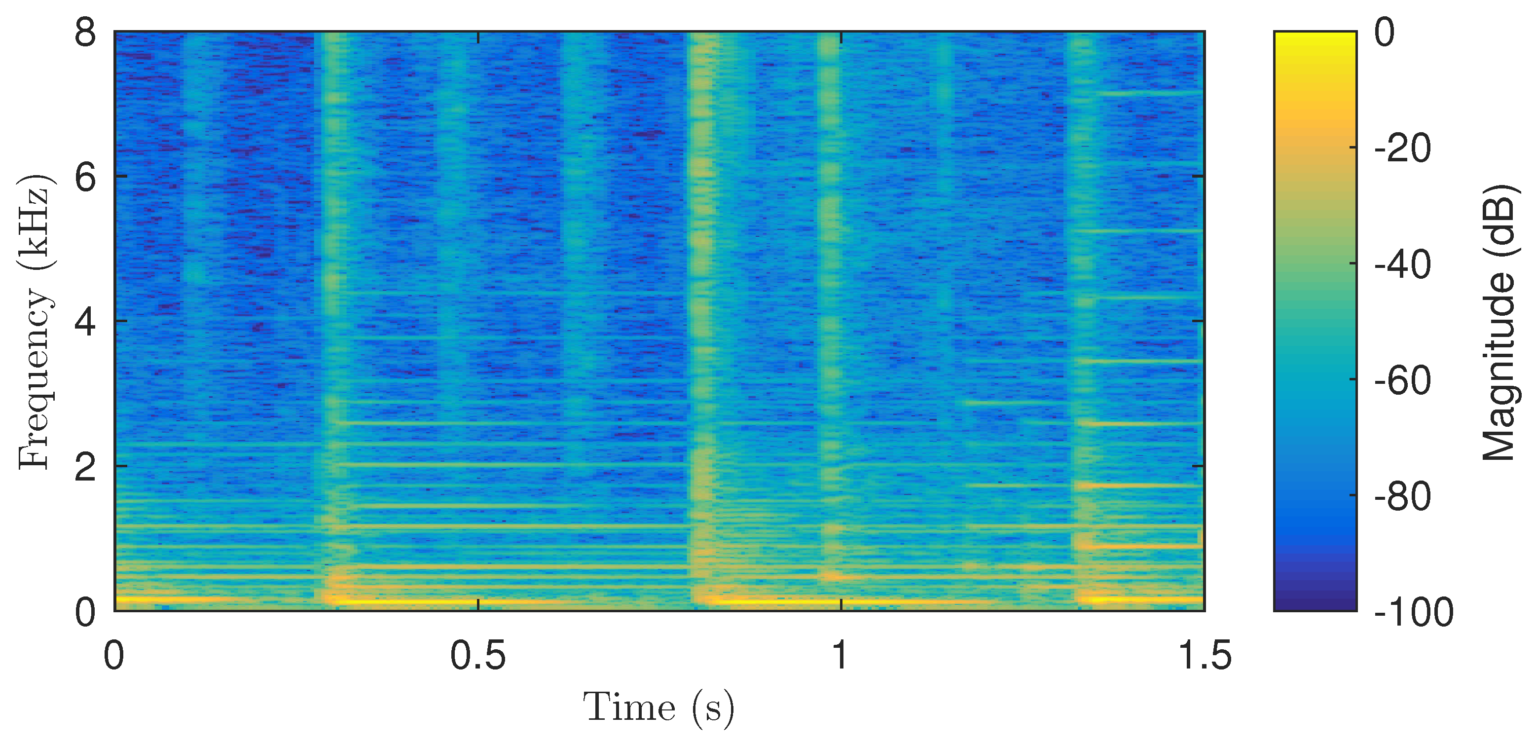
The proposed method for the classification of spectral bins is based on the observation that, in a time-frequency representation of a signal, stationary tonal components appear as ridges in the time direction, whereas transient components appear as ridges in the frequency direction [29,33]. Thus, if a spectral bin contributes to the forming of a time-direction ridge, most of its energy is likely to come from a tonal component in the input signal. Similarly, if a spectral bin contributes to the forming of a frequency-direction ridge, most of its energy is probably from a transient component. As a time-frequency representation, the short-time Fourier transform (STFT) is used:
where m and k are the integer time frame and spectral bin indices, respectively, is the input signal, is the analysis hop size, is the analysis window, N is the analysis frame length and the number of frequency bins in each frame, and is the normalized center frequency of the kth STFT bin. Figure 1 shows the STFT magnitude of a signal consisting of a melody played on the piano, accompanied by soft percussion and a double bass. The time-direction ridges introduced by the harmonic instruments and the frequency-direction ridges introduced by the percussion are apparent on the spectrogram.
The tonal and transient STFTs and , respectively, are computed using the median filtering technique proposed by Fitzgerald [29]:
and
where and are the lengths of the median filters in time and frequency directions, respectively. For the tonal STFT, the subscript s (denoting sinusoidal) is used and for the transient STFT the subscript t. Median filtering in the time direction suppresses the effect of transients in the STFT magnitude, while preserving most of the energy of the tonal components. Conversely, median filtering in the frequency direction suppresses the effect of tonal components, while preserving most of the transient energy [29].
The two median-filtered STFTs are used to estimate the tonalness, noisiness, and transientness of each analysis STFT bin. We estimate tonalness by the ratio
We define transientness as the complement of tonalness:
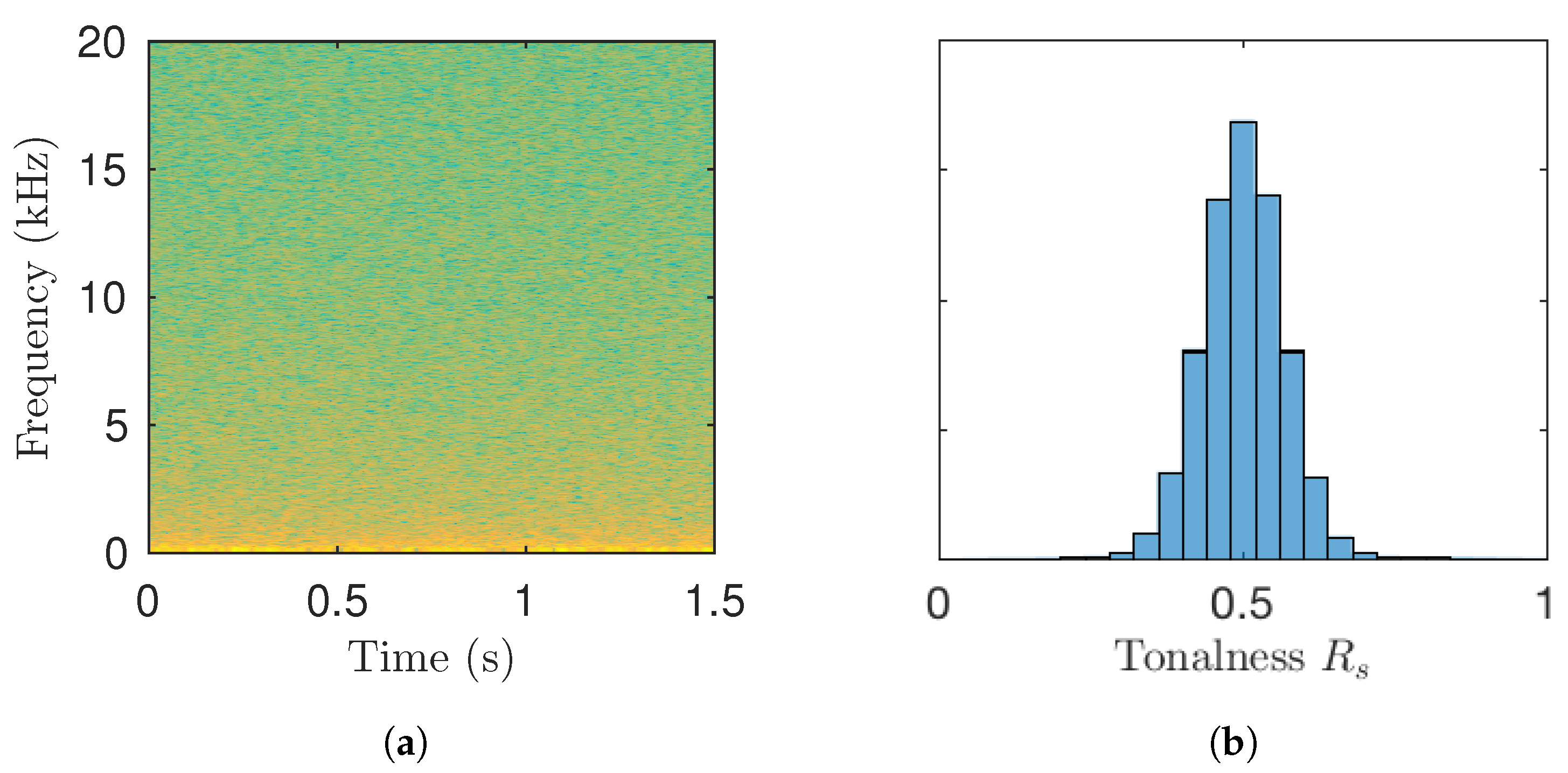
Signal components which are neither tonal nor transient can be assumed to be noiselike. Experiments on noise signal analysis using the above median filtering method show that the tonalness value is often approximately . This is demonstrated in Figure 2b in which a histogram of the tonalness values of STFT bins of a pink noise signal (Figure 2a) is shown. It can be seen that the tonalness values are approximately normally distributed around the value 0.5. Thus, we estimate noisiness by
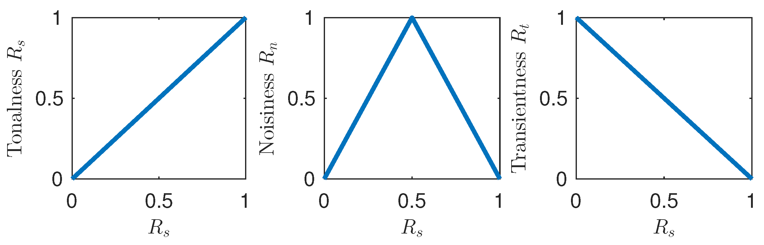
The tonalness, noisiness, and transientness can be used to denote the degree of membership of each STFT bin to the corresponding class in a fuzzy manner. The relations between the classes are visualized in Figure 3.
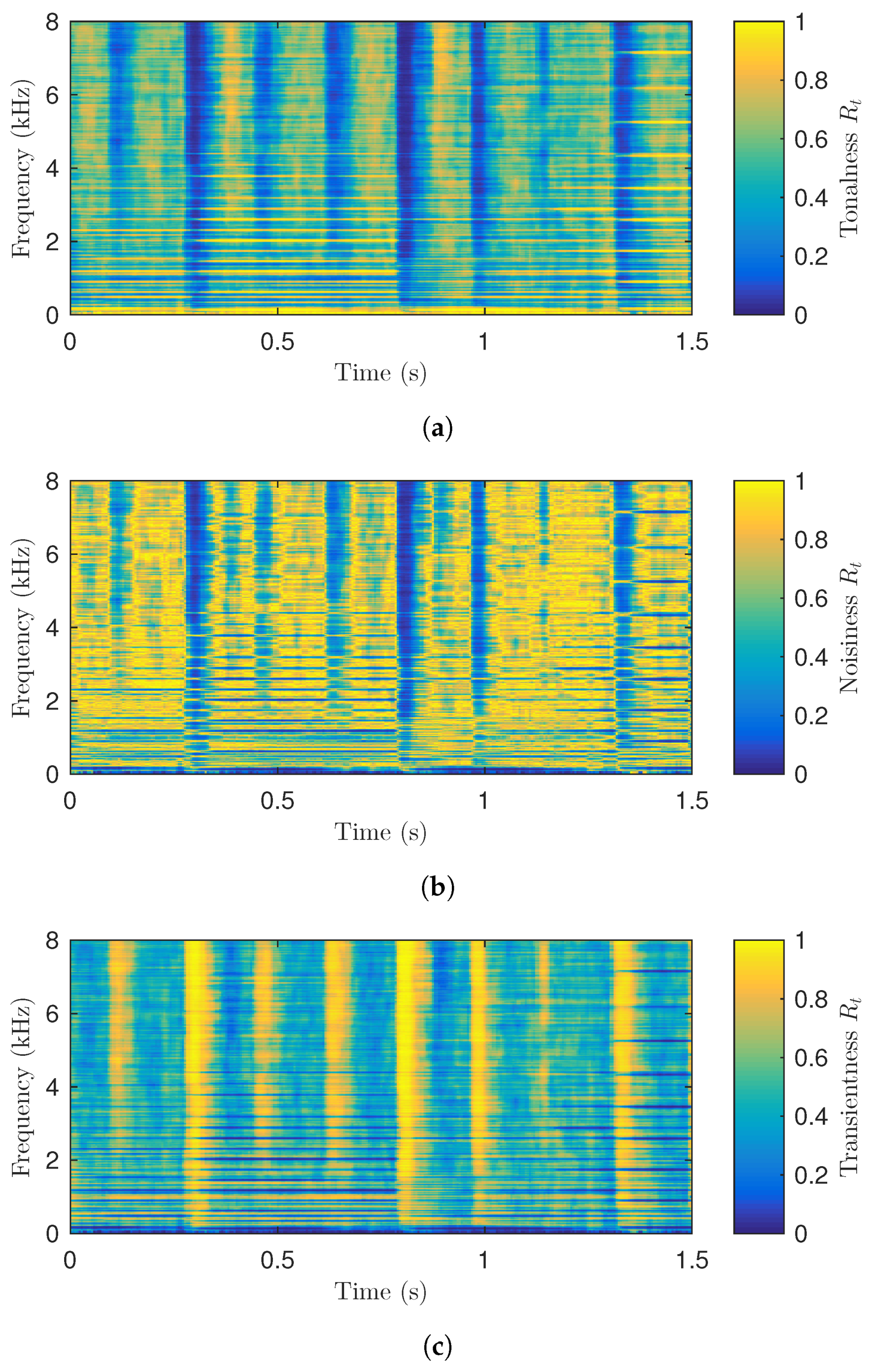
Figure 4 shows the computed tonalness, noisiness, and transientness values for the STFT bins of the example audio signal used above. The tonalness values in Figure 4a are close to 1 for the bins which represent the harmonics of the piano and double bass tones, whereas the tonalness values are close to 0 for the bins which represent percussive sounds. In Figure 4b, the noisiness values are close to 1 for the bins which do not significantly contribute either to the tonal nor the transient components in the input audio. Finally, it can be seen that the transientness values in Figure 4c are complementary to the tonalness values of Figure 4a.
3. Novel Time-Scale Modification Technique
This section introduces the new TSM technique that is based on the fuzzy classification of spectral bins defined above.
3.1. Proposed Phase Propagation
The phase vocoder TSM is based on the differentiation and subsequent integration of the analysis STFT phases in time. This process is known as phase propagation. The phase propagation in the new TSM method is based on a modification to the phase-locked vocoder by Laroche and Dolson [21]. The phase propagation in the phase-locked vocoder can be described as follows. For each frame in the analysis STFT (1), peaks are identified. Peaks are defined as spectral bins, whose magnitude is greater than the magnitude of its four closest neighboring bins.
The phases of the peak bins are differentiated to obtain the instantaneous frequency for each peak bin:
where is the estimated “heterodyned phase increment”:
Here, denotes the principal determination of the angle, i.e., the operator wraps the input angle to the interval . The phases of the peak bins in the synthesis STFT can be computed by integrating the estimated instantaneous frequencies according to the synthesis hop size :
The ratio between the analysis and synthesis hop sizes and determines the TSM factor . In practice, the synthesis hop size is fixed and the analysis hop size then depends on the desired TSM factor:
In the standard phase vocoder TSM [20], the phase propagation of (7)–(9) is applied to all bins, not only peak bins. In the phase-locked vocoder [21], the way the phases of non-peak bins are modified is known as phase locking. It is based on the idea that the phase relations between all spectral bins, which contribute to the representation of a single sinusoid, should be preserved when the phases are modified. This is achieved by modifying the phases of the STFT bins surrounding each peak such that the phase relations between the peak and the surrounding bins are preserved from the analysis STFT. Given a peak bin , the phases of the bins surrounding the peak are modified by:
where is computed according to (7)–(9). This approach is known as identity phase locking.
As the motivation behind phase locking states, it should only be applied to bins that are considered sinusoidal. When applied to non-sinusoidal bins, the phase locking introduces a metallic sounding artifact to the processed signal. Since the tonalness, noisiness, and transientness of each bin are determined, this information can be used when the phase locking is applied. We want to be able to apply phase locking to bins which represent a tonal component, while preserving the randomized phase relationships of bins representing noise.
Thus, the phase locking is first applied to all bins. Afterwards, phase randomization is applied to the bins according to the estimated noisiness values. The final synthesis phases are obtained by adding uniformly distributed noise to the synthesis phases computed with the phase-locked vocoder:
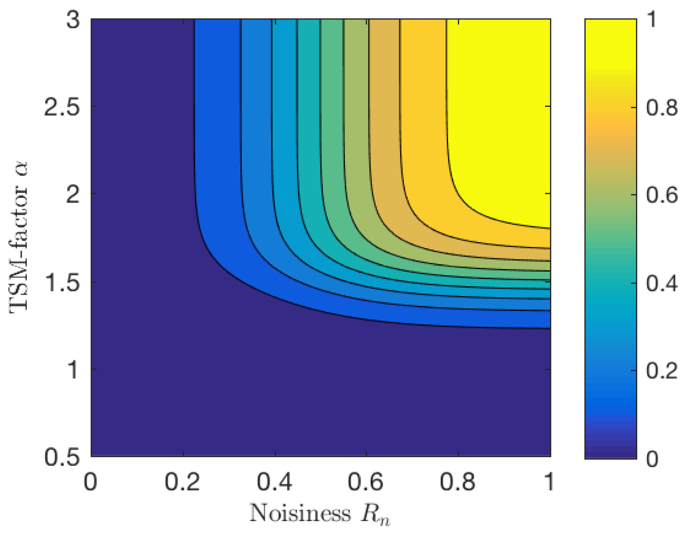
where are the added noise values and are the synthesis phases computed with the phase-locked vocoder. The pseudo-random numbers are drawn from the uniform distribution . is the phase randomization factor, which is based on the estimated noisiness of the bin and the TSM factor :
where constants and control the shape of non-linear mappings of the hyperbolic tangents. The values were used in this implementation.
The phase randomization factor , as a function of the estimated noisiness and the TSM factor , is shown in Figure 5. The phase randomization factor increases with increasing TSM factor and noisiness. The phase randomization factor saturates as the values increase, so that at most, the uniform noise added to the phases obtains values in the interval .
3.2. Transient Detection and Preservation
For transient detection and preservation, a similar strategy to [23] was adopted. However, the proposed method is based on the estimated transientness of the STFT bins. Using the measure for transientness, the smearing of both the transient onsets and offsets is prevented. The transients are processed so that the transient energy is mostly contained on a single synthesis frame, effectively suppressing the transient smearing artifact, which is typical for the phase vocoder based TSM.
3.2.1. Detection
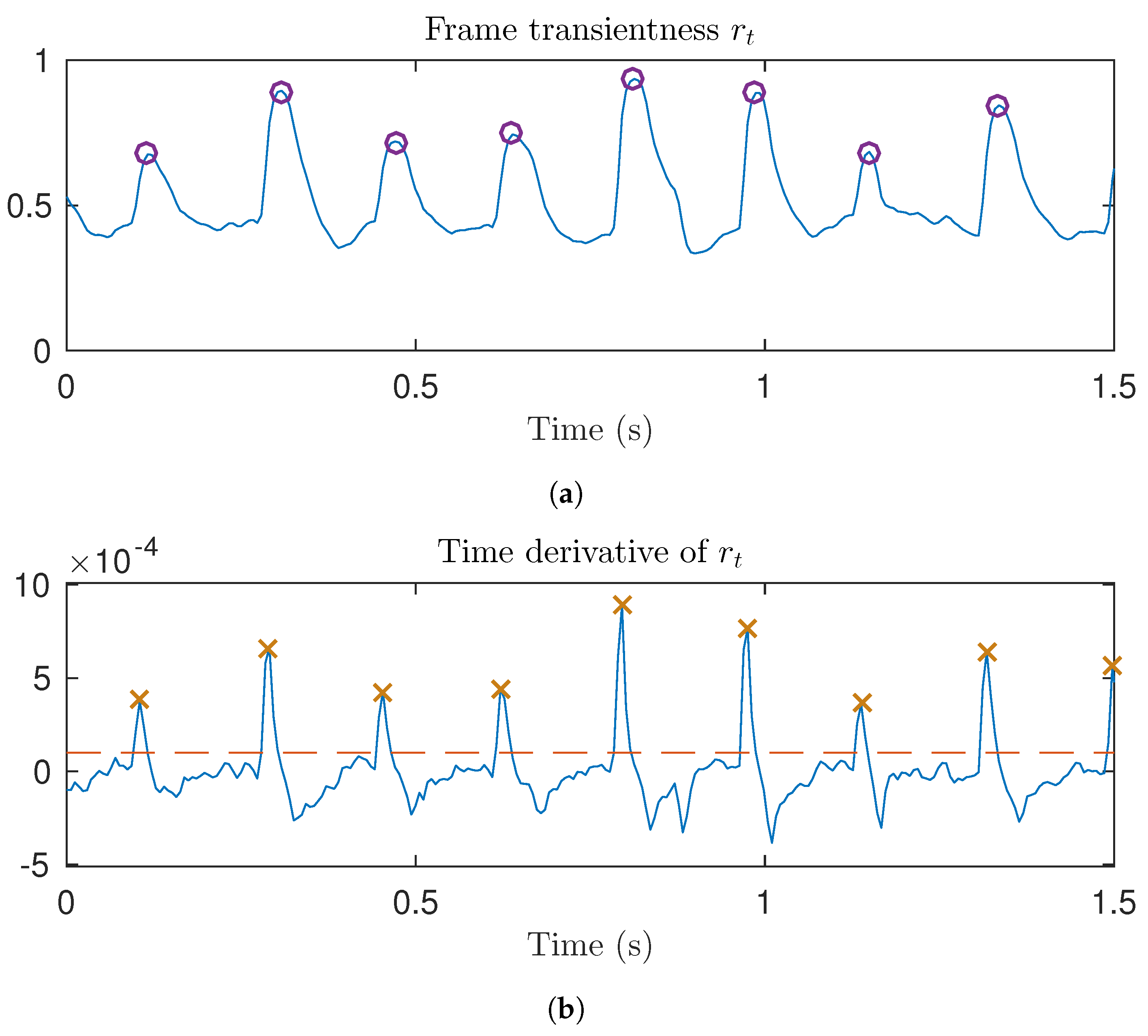
To detect transients, the overall transientness of each analysis frame is estimated, and denoted as frame transientness:
The analysis frames which are centered on a transient component appear as local maxima in the frame transientness. Transients need to be detected as soon as the analysis window slides over them in order to prevent the smearing of transient onsets. To this end, the time derivative of frame transientness is used:
where the time derivative is approximated with the backward difference method. As the analysis window slides over a transient, there is an abrupt increase in the frame transientness. These instants appear as local maxima in the time derivative of the frame transientness. Local maxima in the time derivative of the frame transientness that exceed a given threshold are used for transient detection.
Figure 6 illustrates the proposed transient detection method using the same audio excerpt as above, containing piano, percussion, and double bass. The transients appear as local maxima in the frame transientness signal in Figure 6a. Transient onsets are detected from the time derivative of the frame transientness, from the local maxima, which exceed the given threshold (the red dashed line in Figure 6b). The detected transient onsets are marked with orange crosses. After an onset is detected, the analysis frame which is centered on the transient is detected from the subsequent local maxima in the frame transientness. The detected analysis frames centered on a transient are marked with purple circles in Figure 6a.
3.2.2. Transient Preservation
To prevent transient smearing, it is necessary to concentrate the transient energy in time. A single transient contributes energy to multiple analysis frames, because the frames are overlapping. During the synthesis, the phases of the STFT bins are modified, and the synthesis frames are relocated in time, which results in smearing of the transient energy.
To remove this effect, transients are detected as the analysis window slides over them. When a transient onset has been detected using the method described above, the energy in the STFT bins is suppressed according to their estimated transientness:
This gain is only applied to bins whose estimated transientness is larger than 0.5. Similar to [23], the bins to which this gain has been applied are kept in a non-contracting set of transient bins . When it is detected that the analysis window is centered on a transient, as explained above, a phase reset is performed on the transient bins. That is, the original analysis phases are kept during synthesis for the transient bins. Subsequently, as the analysis window slides over the transient, the same gain reduction is applied for the transient bins, as during the onset of the transient (16). The bins are retained in the set of transient bins until their transientness decays to a value smaller than 0.5, or until the analysis frame slides completely away from the detected transient center. Finally, since the synthesis frames before and after the center of the transient do not contribute to the transients’ energy, the magnitudes of the transient bins are compensated by
where is the transient frame index, denotes the number of elements in the set , and , which is the defined set of transient bins.
This method aims to prevent the smearing of both the transient onsets and offsets during TSM. In effect, the transients are separated from the input audio, and relocated in time according to the TSM factor. However, in contrast to methods where transients are explicitly separated from the input audio [13,14,28,34], the proposed method is more likely to keep transients perceptually intact with other components of the sound. Since the transients are kept in the same STFT representation, phase modifications in subsequent frames are dependent on the phases of the transient bins. This suggests that transients related to the onsets of harmonic sounds, such as the pluck of a note while strumming a guitar, should blend smoothly with the following tonal component of the sound. Furthermore, the soft manner in which the amplitudes of the transient bins are attenuated during onsets and offsets should prevent strong artifacts arising from errors in the transient detection.
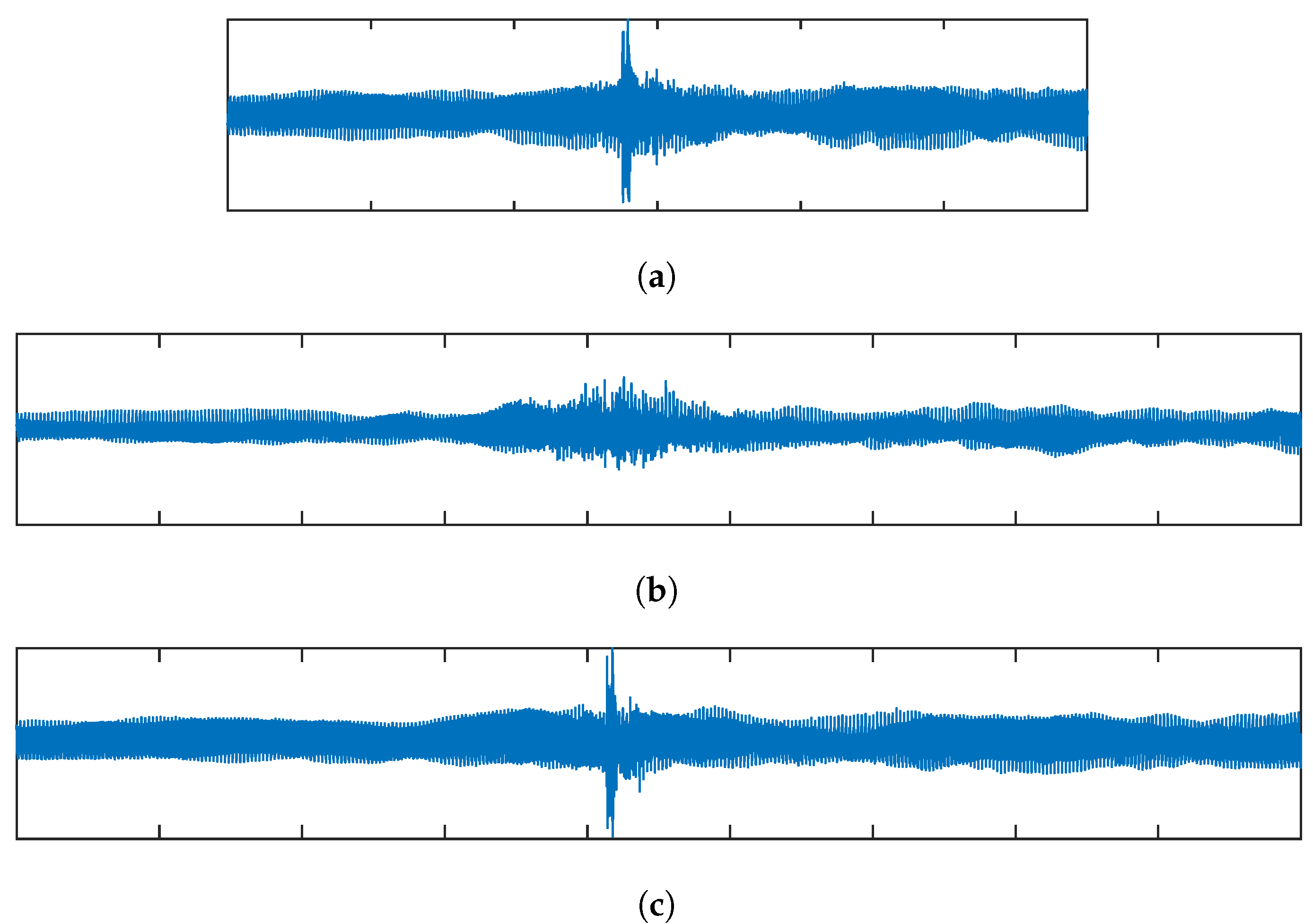
Figure 7 shows an example of a transient processed with the proposed method. The original audio shown in Figure 7a consists of a solo violin overlaid with a castanet click. Figure 7b shows the time-scale modified sample with TSM factor , using the standard phase vocoder. In the modified sample, the energy of the castanet click is spread over time. This demonstrates the well known transient smearing artifact of standard phase vocoder TSM. Figure 7c shows the time-scale modified sample using the proposed method. It can be seen that while the duration of the signal has changed, the castanet click in the modified audio resembles the one in the original, without any visible transient smearing.
4. Evaluation
To evaluate the quality of the proposed TSM technique, a listening test was conducted. The listening test was realized online using the Web Audio Evaluation Tool [35]. The test subjects were asked to use headphones. The test setup used was the same as in [28]. In each trial, the subjects were presented with the original audio sample and four modified samples processed with different TSM techniques. The subjects were asked to rate the quality of time-scale modified audio excerpts using a scale from 1 (poor) to 5 (excellent).
All 11 subjects who participated in the test reported having a background in acoustics, and 10 of them had previous experience of participating in listening tests. None of the subjects reported hearing problems. The ages of the subjects ranged from 23 to 37, with a median age of 28. Of the 11 subjects, 10 were male and 1 was female.
In the evaluation of the proposed method, the following settings were used: the sample rate was 44.1 kHz, a Hann window of length was chosen for the STFT analysis and synthesis, the synthesis hop size was set to , and the number of frequency bins in the STFT was . The length of the median filter in the frequency direction was 500 Hz, which corresponds to 46 bins. In the time direction, the length of the median filter was chosen to be 200 ms, but the number of frames it corresponds to depends on the analysis hop size, which is determined by the TSM factor according to (10). Finally, the transient detection threshold was set to .
In addition to the proposed method (PROP), the following techniques were included: the standard phase vocoder (PV), using the same STFT analysis and synthesis settings as the proposed method; a recently published technique (harmonic–percussive separation, HP) [28], which uses harmonic and percussive separation for transient preservation; and the élastique algorithm (EL) [36], which is a state-of-the-art commercial tool for time and pitch-scale modification. The samples processed by these methods were obtained using the TSM toolbox [37].
Eight different audio excerpts (sampled at 44.1 kHz) and two different stretching factors and were tested using the four techniques. This resulted in a total of 64 samples rated by each subject. The audio excerpts are described in Table 1. The lengths of the original audio excerpts ranged from 3 to 10 s. The processed audio excerpts and Matlab code for the proposed method are available online at http://research.spa.aalto.fi/publications/papers/applsci-ats/.
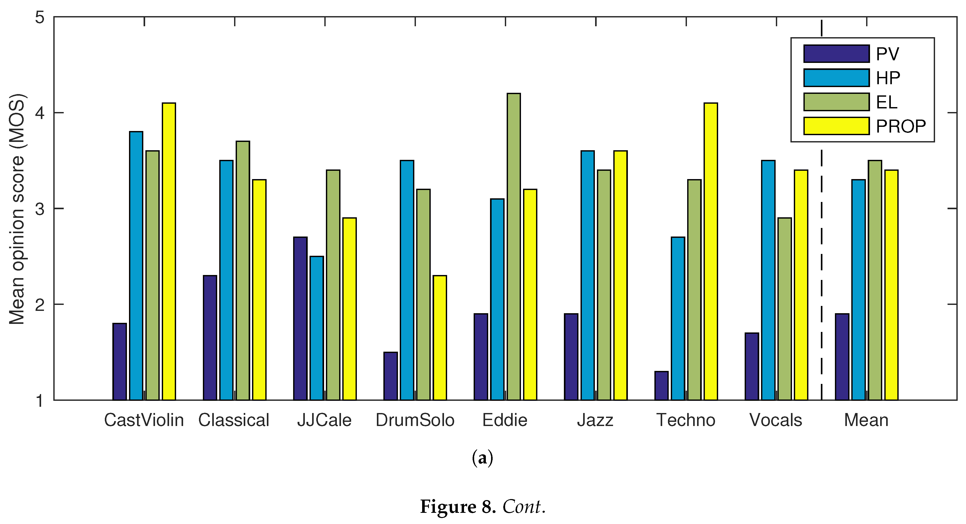
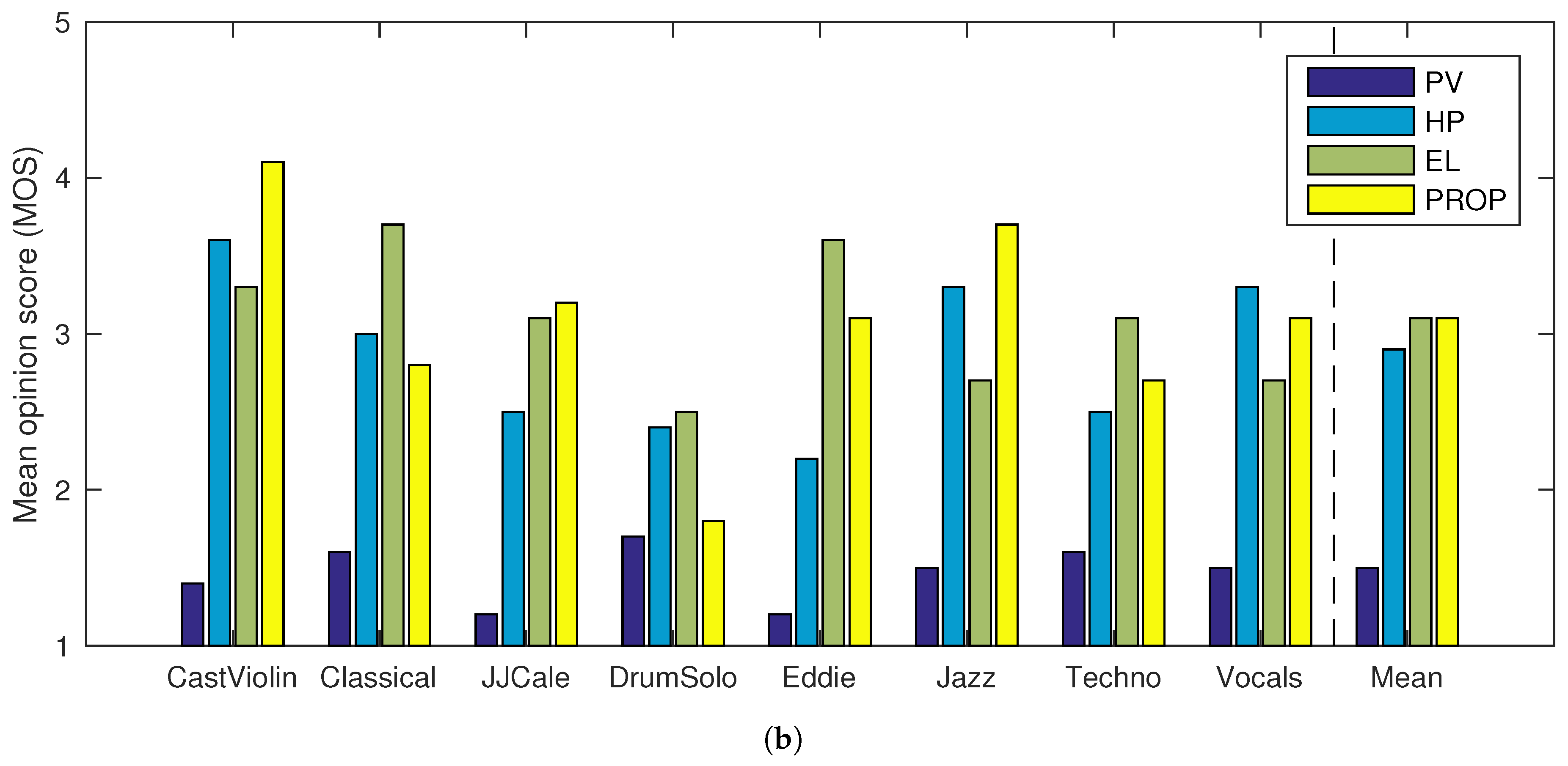
To estimate the sound quality of the techniques, mean opinion scores (MOS) were computed for all samples from the ratings given by the subjects. The resulting MOS values are shown in Table 2. A bar diagram of the same data is also shown in Figure 8.
As expected, the standard PV performed worse than all the other tested methods. For the CastViolin sample, the proposed method (PROP) performed better than the other methods, with both TSM factors. This suggests that the proposed method preserves the quality of the transients in the modified signals better than the other methods. The proposed method also scored best with the Jazz excerpt. In addition to the well-preserved transients, the results are likely to be explained by the naturalness of the singing voice in the modified signals. This can be attributed to the proposed phase propagation, which allows simultaneous preservation of the tonal and noisy qualities of the singing voice. This is also reflected in the results of the Vocals excerpt, where the proposed method also performed well, while scoring slightly lower than HP. For the Techno sample, the proposed method scored significantly higher than the other methods with TSM factor . For TSM factor , however, the proposed method scored lower than EL. The proposed method also scored highest for the JJCale sample with TSM factor .
The proposed method performed more poorly on the excerpts DrumSolo and Classical. Both of these samples contained fast sequences of transients. It is likely that the poorer performance is due to the individual transients not being resolved during the analysis, because of the relatively long analysis window used. Also, for the excerpt Eddie, EL scored higher than the proposed method. Note that the audio excepts were not selected so that the results would be preferable for one of the tested methods. Instead, they represent some interesting and critical cases, such as singing and sharp transients.
The preferences of subjects over the tested TSM methods seem to depend significantly on the signal being processed. Overall, the MOS values computed from all the samples suggest that the proposed method yields slightly better quality than HP and practically the same quality as EL.
The proposed method introduces some additional computational complexity when compared to the standard phase-locked vocoder. In the analysis stage, the fuzzy classification of the spectral bins requires median filtering of the magnitude of the analysis STFT. The number of samples in each median filtering operation depends on the analysis hop size and the number of frequency bins in each short time spectra. In the modification stage, additional complexity arises from drawing pseudo-random values for the phase randomization. Furthermore, computing the phase randomization factor, as in Equation (13), requires the evaluation of two hyperbolic tangent functions for each point in the STFT. Since the argument for the second hyperbolic tangent depends only on the TSM factor, its value needs to be updated only when the TSM factor is changed. Finally, due to the way the values are used, a lookup table approximation can be used for evaluating the hyperbolic tangents without significantly affecting the quality of the modification.
5. Conclusions
In this paper, a novel TSM method was presented. The method is based on fuzzy classification of spectral bins into sinusoids, noise, and transients. The information from the bin classification is used to preserve the characteristics of these distinct signal components during TSM. The listening test results presented in this paper suggest that the proposed method performs generally better than a state-of-the-art algorithm and is competitive with commercial software.
The proposed method still suffers to some extent from the fixed time and frequency resolution of the STFT. Finding ways to apply the concept of fuzzy classification of spectral bins to a multiresolution time-frequency transformation could further increase the quality of the proposed method. Finally, although this paper only considered TSM, the method for fuzzy classification of spectral bins could be applied to various audio signal analysis tasks, such as multi-pitch estimation and beat tracking.
Acknowledgments
This study has been funded by the Aalto University School of Electrical Engineering. Special thanks go to the experience director of the Finnish Science Center Heureka Mikko Myllykoski, who proposed this study. The authors would also like to thank Mr. Etienne Thuillier for providing expert help in the beginning of this project, and Craig Rollo for proofreading.
Author Contributions
E.P.D. and V.V. planned this study and wrote the paper together. E.P.D. developed and programmed the new algorithm. E.P.D. conducted the listening test and analyzed the results. V.V. supervised this work.
Conflicts of Interest
The authors declare no conflict of interest.
References
- Moulines, E.; Laroche, J. Non-parametric techniques for pitch-scale and time-scale modification of speech. Speech Commun. 1995, 16, 175–205. [Google Scholar] [CrossRef]
- Barry, D.; Dorran, D.; Coyle, E. Time and pitch scale modification: A real-time framework and tutorial. In Proceedings of the International Conference on Digital Audio Effects (DAFx), Espoo, Finland, 1–4 September 2008; pp. 103–110. [Google Scholar]
- Driedger, J.; Müller, M. A review of time-scale modification of music signals. Appl. Sci. 2016, 6, 57. [Google Scholar] [CrossRef]
- Amir, A.; Ponceleon, D.; Blanchard, B.; Petkovic, D.; Srinivasan, S.; Cohen, G. Using audio time scale modification for video browsing. In Proceedings of the 33rd Annual Hawaii International Conference on System Sciences (HICSS), Maui, HI, USA, 4–7 January 2000. [Google Scholar]
- Cliff, D. Hang the DJ: Automatic sequencing and seamless mixing of dance-music tracks. In Technical Report; Hewlett-Packard Laboratories: Bristol, UK, 2000; Volume 104. [Google Scholar]
- Donnellan, O.; Jung, E.; Coyle, E. Speech-adaptive time-scale modification for computer assisted language-learning. In Proceedings of the Third IEEE International Conference on Advanced Learning Technologies, Athens, Greece, 9–11 July 2003; pp. 165–169. [Google Scholar]
- Dutilleux, P.; De Poli, G.; von dem Knesebeck, A.; Zölzer, U. Time-segment processing (chapter 6). In DAFX: Digital Audio Effects, Second Edition; Zölzer, U., Ed.; Wiley: Chichester, UK, 2011; pp. 185–217. [Google Scholar]
- Moinet, A.; Dutoit, T.; Latour, P. Audio time-scaling for slow motion sports videos. In Proceedings of the International Conference on Digital Audio Effects (DAFx), Maynooth, Ireland, 2–5 September 2013; pp. 314–320. [Google Scholar]
- Haghparast, A.; Penttinen, H.; Välimäki, V. Real-time pitch-shifting of musical signals by a time-varying factor using normalized filtered correlation time-scale modification (NFC-TSM). In Proceedings of the International Conference on Digital Audio Effects (DAFx), Bordeaux, France, 10–15 September 2007; pp. 7–13. [Google Scholar]
- Santacruz, J.; Tardón, L.; Barbancho, I.; Barbancho, A. Spectral envelope transformation in singing voice for advanced pitch shifting. Appl. Sci. 2016, 6, 368. [Google Scholar] [CrossRef]
- Verma, T.S.; Meng, T.H. An analysis/synthesis tool for transient signals that allows a flexible sines+transients+noise model for audio. In Proceedings of the IEEE International Conference on Acoustics, Speech and Signal Processing (ICASSP), Las Vegas, NV, USA, 30 March–4 April 1998; pp. 3573–3576. [Google Scholar]
- Levine, S.N.; Smith, J.O., III. A sines+transients+noise audio representation for data compression and time/pitch scale modifications. In Proceedings of the Audio Engineering Society 105th Convention, San Francisco, CA, USA, 26–29 September 1998. [Google Scholar]
- Verma, T.S.; Meng, T.H. Time scale modification using a sines+transients+noise signal model. In Proceedings of the Digital Audio Effects Workshop (DAFx), Barcelona, Spain, 19–21 November 1998. [Google Scholar]
- Verma, T.S.; Meng, T.H. Extending spectral modeling synthesis with transient modeling synthesis. Comput. Music J. 2000, 24, 47–59. [Google Scholar] [CrossRef]
- Roucos, S.; Wilgus, A. High quality time-scale modification for speech. In Proceedings of the IEEE International Conference on Acoustics, Speech, and Signal Processing (ICASSP), Tampa, FL, USA, 26–29 April 1985; Volume 10, pp. 493–496. [Google Scholar]
- Verhelst, W.; Roelands, M. An overlap-add technique based on waveform similarity (WSOLA) for high quality time-scale modification of speech. In Proceedings of the IEEE International Conference on Acoustics, Speech, and Signal Processing (ICASSP), Minneapolis, MN, USA, 27–30 April 1993; pp. 554–557. [Google Scholar]
- Moulines, E.; Charpentier, F. Pitch-synchronous waveform processing techniques for text-to-speech synthesis using diphones. Speech Commun. 1990, 9, 453–467. [Google Scholar] [CrossRef]
- Lee, S.; Kim, H.D.; Kim, H.S. Variable time-scale modification of speech using transient information. In Proceedings of the IEEE International Conference on Acoustics, Speech, and Signal Processing (ICASSP), Münich, Germany, 21–24 April 1997; Volume 2, pp. 1319–1322. [Google Scholar]
- Wong, P.H.; Au, O.C.; Wong, J.W.; Lau, W.H. On improving the intelligibility of synchronized over-lap-and-add (SOLA) at low TSM factor. In Proceedings of the IEEE Region 10 Annual Conference on Speech and Image Technologies for Computing and Telecommunications (TENCON), Brisbane, Australia, 2–4 December 1997; Volume 2, pp. 487–490. [Google Scholar]
- Portnoff, M. Time-scale modification of speech based on short-time Fourier analysis. IEEE Trans. Acoust. Speech Signal Process. 1981, 29, 374–390. [Google Scholar] [CrossRef]
- Laroche, J.; Dolson, M. Improved phase vocoder time-scale modification of audio. IEEE Trans. Speech Audio Process. 1999, 7, 323–332. [Google Scholar] [CrossRef]
- Laroche, J.; Dolson, M. Phase-vocoder: About this phasiness business. In Proceedings of the IEEE ASSP Workshop on Applications of Signal Processing to Audio and Acoustics, New Paltz, NY, USA, 19–22 October 1997. [Google Scholar]
- Röbel, A. A new approach to transient processing in the phase vocoder. In Proceedings of the 6th International Conference on Digital Audio Effects (DAFx), London, UK, 8–11 September 2003; pp. 344–349. [Google Scholar]
- Bonada, J. Automatic technique in frequency domain for near-lossless time-scale modification of audio. In Proceedings of the International Computer Music Conference (ICMC), Berlin, Germany, 27 August–1 September 2000; pp. 396–399. [Google Scholar]
- Duxbury, C.; Davies, M.; Sandler, M.B. Improved time-scaling of musical audio using phase locking at transients. In Proceedings of the Audio Engineering Society 112th Convention, München, Germany, 10–13 May 2002. [Google Scholar]
- Röbel, A. A shape-invariant phase vocoder for speech transformation. In Proceedings of the International Conference on Digital Audio Effects (DAFx), Graz, Austria, 6–10 September 2010; pp. 298–305. [Google Scholar]
- Zivanovic, M.; Röbel, A.; Rodet, X. Adaptive threshold determination for spectral peak classification. Comput. Music J. 2008, 32, 57–67. [Google Scholar] [CrossRef]
- Driedger, J.; Müller, M.; Ewert, S. Improving time-scale modification of music signals using harmonic-percussive separation. IEEE Signal Process. Lett. 2014, 21, 105–109. [Google Scholar] [CrossRef]
- Fitzgerald, D. Harmonic/percussive separation using median filtering. In Proceedings of the International Conference on Digital Audio Effects (DAFx), Graz, Austria, 6–10 September 2010; pp. 217–220. [Google Scholar]
- Zadeh, L.A. Making computers think like people. IEEE Spectr. 1984, 21, 26–32. [Google Scholar] [CrossRef]
- Del Amo, A.; Montero, J.; Cutello, V. On the principles of fuzzy classification. In Proceedings of the 18th International Conference of the North American Fuzzy Information Processing Society, New York, NY, USA, 10–12 June 1999; pp. 675–679. [Google Scholar]
- Kraft, S.; Lerch, A.; Zölzer, U. The tonalness spectrum: Feature-based estimation of tonal components. In Proceedings of the International Conference on Digital Audio Effects (DAFx), Maynooth, Ireland, 2–5 September 2013; pp. 17–24. [Google Scholar]
- Ono, N.; Miyamoto, K.; Le Roux, J.; Kameoka, H.; Sagayama, S. Separation of a monaural audio signal into harmonic/percussive components by complementary diffusion on spectrogram. In Proceedings of the European Signal Processing Conference (EUSIPCO), Lausanne, Switzerland, 25–29 August 2008; pp. 1–4. [Google Scholar]
- Nagel, F.; Walther, A. A novel transient handling scheme for time stretching algorithms. In Proceedings of the Audio Engineering Society 127th Convention, New York, NY, USA, 9–12 October 2009. [Google Scholar]
- Jillings, N.; Moffat, D.; De Man, B.; Reiss, J.D. Web Audio Evaluation Tool: A browser-based listening test environment. In Proceedings of the 12th Sound and Music Computing Conference, Maynooth, Ireland, 26 July–1 August 2015; pp. 147–152. [Google Scholar]
- Zplane Development. Élastique Time Stretching & Pitch Shifting SDKs. Available online: http://www.zplane.de/index.php?page=description-elastique (accessed on 20 October 2017).
- Driedger, J.; Müller, M. TSM toolbox: MATLAB implementations of time-scale modification algorithms. In Proceedings of the International Conference on Digital Audio Effects (DAFx), Erlangen, Germany, 1–5 September 2014; pp. 249–256. [Google Scholar]
Figure 1.
Spectrogram of a signal consisting of piano, percussion, and double bass.

Figure 2.
(a) Spectrogram of pink noise and (b) the histogram of tonalness values for its spectrogram bins.
Figure 2.
(a) Spectrogram of pink noise and (b) the histogram of tonalness values for its spectrogram bins.

Figure 3.
The relations between the three fuzzy classes.

Figure 4.
(a) Tonalness, (b) noisiness, and (c) transientness values for the short-time Fourier transform (STFT) bins of the example audio signal. Cf. Figure 1.
Figure 4.
(a) Tonalness, (b) noisiness, and (c) transientness values for the short-time Fourier transform (STFT) bins of the example audio signal. Cf. Figure 1.

Figure 5.
A contour plot of the phase randomization factor , with . TSM: time-scale modification.

Figure 6.
Illustration of the proposed transient detection. (a) Frame transientness. Locations of the detected transients are marked with purple circles; (b) Time derivative of the frame transientness. Detected transient onsets are marked with orange crosses. The red dashed line shows the transient detection threshold.

Figure 7.
An example of the proposed transient preservation method. (a) shows the original audio, consisting of a solo violin overlaid with a castanet click. Also shown are the modified samples with TSM factor , using (b) the standard phase vocoder, and (c) the proposed method.
Figure 7.
An example of the proposed transient preservation method. (a) shows the original audio, consisting of a solo violin overlaid with a castanet click. Also shown are the modified samples with TSM factor , using (b) the standard phase vocoder, and (c) the proposed method.

Figure 8.
Mean opinion scores for eight audio samples using four TSM methods for (a) medium (), and (b) large () TSM factors. The rightmost bars show the average score for all eight samples. PV: phase vocoder; HP: harmonic–percussive separation [28]; EL: élastique [36]; PROP: proposed method.


Table 1.
List of audio excerpts used in the subjective listening test.
| Name | Description |
|---|---|
| CastViolin | Solo violin and castanets, from [37] |
| Classical | Excerpt from Bólero, performed by the London Symphony Orchestra |
| JJCale | Excerpt from Cocaine, performed by J.J. Cale |
| DrumSolo | Solo performed on a drum set, from [37] |
| Eddie | Excerpt from Early in the Morning, performed by Eddie Rabbit |
| Jazz | Excerpt from I Can See Clearly, performed by the Holly Cole Trio |
| Techno | Excerpt from Return to Balojax, performed by Deviant Species and Scorb |
| Vocals | Excerpt from Tom’s Diner, performed by Suzanne Vega |
Table 2.
Mean opinion scores for the audio samples. PV: phase vocoder; HP: harmonic–percussive separation; EL: élastique algorithm; PROP: proposed method.
Table 2.
Mean opinion scores for the audio samples. PV: phase vocoder; HP: harmonic–percussive separation; EL: élastique algorithm; PROP: proposed method.
| PV | HP | EL | PROP | PV | HP | EL | PROP | |
|---|---|---|---|---|---|---|---|---|
| CastViolin | 1.8 | 3.8 | 3.6 | 4.1 | 1.4 | 3.6 | 3.3 | 4.1 |
| Classical | 2.3 | 3.5 | 3.7 | 3.3 | 1.6 | 3.0 | 3.7 | 2.8 |
| JJCale | 2.7 | 2.5 | 3.4 | 2.9 | 1.2 | 2.5 | 3.1 | 3.2 |
| DrumSolo | 1.5 | 3.5 | 3.2 | 2.3 | 1.7 | 2.4 | 2.5 | 1.8 |
| Eddie | 1.9 | 3.1 | 4.2 | 3.2 | 1.2 | 2.2 | 3.6 | 3.1 |
| Jazz | 1.9 | 3.6 | 3.4 | 3.6 | 1.5 | 3.3 | 2.7 | 3.7 |
| Techno | 1.3 | 2.7 | 3.3 | 4.1 | 1.6 | 2.5 | 3.1 | 2.7 |
| Vocals | 1.7 | 3.5 | 2.9 | 3.4 | 1.5 | 3.3 | 2.7 | 3.1 |
| Mean | 1.9 | 3.3 | 3.5 | 3.4 | 1.5 | 2.9 | 3.1 | 3.1 |
© 2017 by the authors. Licensee MDPI, Basel, Switzerland. This article is an open access article distributed under the terms and conditions of the Creative Commons Attribution (CC BY) license (http://creativecommons.org/licenses/by/4.0/).
Share and Cite
MDPI and ACS Style
Damskägg, E.-P.; Välimäki, V. Audio Time Stretching Using Fuzzy Classification of Spectral Bins. Appl. Sci. 2017, 7, 1293. https://doi.org/10.3390/app7121293
AMA Style
Damskägg E-P, Välimäki V. Audio Time Stretching Using Fuzzy Classification of Spectral Bins. Applied Sciences. 2017; 7(12):1293. https://doi.org/10.3390/app7121293
Chicago/Turabian StyleDamskägg, Eero-Pekka, and Vesa Välimäki. 2017. "Audio Time Stretching Using Fuzzy Classification of Spectral Bins" Applied Sciences 7, no. 12: 1293. https://doi.org/10.3390/app7121293
Note that from the first issue of 2016, this journal uses article numbers instead of page numbers. See further details here.