An Explicit Approach Toward Modeling Thermo-Coupled Deformation Behaviors of SMPs

Abstract

A new elastoplastic $J_2$-flow models with thermal effects is proposed toward simulating thermo-coupled finite deformation behaviors of shape memory polymers. In this new model, an elastic potential evolving with development of plastic flow is incorporated to characterize the stress-softening effect at unloading and, moreover, thermo-induced plastic flow is introduced to represent the strain recovery effect at heating. It is shown that any given test data for both effects may be accurately simulated by means of direct and explicit procedures. Numerical examples for model predictions compare well with test data in literature.

1. Motivation and Introduction

In recent years, much attention has been directed to smart materials such as shape memory alloys (SMAs) and shape memory polymers (SMPs) (cf., e.g., [1,2]). It is of great interest to simulate thermo-coupled deformation behaviors of such materials under both loading and heating. Unlike deformation behavior of SMAs with very small elastic deformations, however, SMPs exhibit complicated thermo-mechanical deformation effects coupled with both temperature and large recoverable deformations. Typical representatives of such effects are the stress softening effect at unloading in the isothermal case and the strain recovery effect at pure heating. The former is characteristic of all kinds of polymers and associated with a number of unloading stress-strain curves of complex shapes that differ from one another and result in different permanent sets, while the latter is unique to SMPs and related to the recovery of a large pre-strain at heating. Usually, recoverable strains of SMPs both at unloading and at heating may be several hundred percents. As such, large thermo-coupled inelastic deformations incorporating large recoverable deformations should be treated toward modeling thermo-mechanical behavior of SMPs, in particular, in simulating both the stress-softening effect at unloading and the large strain recovery effect at heating (i.e., the shape memory effect).

Many efforts have been made to establish constitutive models for the purpose of incorporating the above two effects. As a typical isothermal deformation feature for various kinds of polymers, the stress softening effect at unloading was observed earlier and has been simulated for some time. Results in this respect have been given based either on phenomenological models with damage-like variables or micro-mechanical models with macromolecular mechanisms. Representatives in these respects may be found, e.g., earlier in [3] and later in [4,5,6,7,8,9,10,11,12,13,14] for phenomenological models, and in [15,16,17,18,19,20,21,22,23,24,25] for micro-mechanical models. On the other side, the modeling of the shape memory effect for SMPs is relatively recent. Results in this respect and, generally, in the thermo-mechanical behavior of SMPs may be found, e.g., in [26,27,28,29,30,31,32,33,34,35,36,37,38,39] and many others.

In the existing models, usually a large number of parameters should be introduced from various standpoints. For a given material sample, in order to find out suitable values of these parameters, complicated numerical procedures should be iteratively carried out to obtain model predictions for stress, strain and temperature from a constitutive model consisting of several nonlinear differential equations, until such parameter values are found that the model predictions with these values fit test data given for this sample as closely as possible. Undue complexities would be expected in identifying a large number of parameters coupled with one another. In particular, that may be the case in fitting a number of unloading curves of different shapes. Even if the model applicability is validated for a material sample, it may not be clear that that will be the case for another material sample. Moreover, both the stress softening effect and the shape memory effect are usually treated separately and could not be simultaneously simulated in a unified and accurate sense.

In this contribution, we are going to propose an explicit, direct approach toward modeling thermo-mechanical behavior of SMPs. It is shown that finite thermo-coupled inelastic deformation behavior of SMPs may be simulated by establishing new finite elastoplastic $J_2$-flow models with thermo-coupled effects. In particular, both the stress softening effect at unloading and the shape memory effect at heating may be derived from the proposed model. The main idea is incorporation of an elastic potential evolving with development of plastic flow and introduction of thermo-induced plastic flow, as suggested in a previous study for polymeric solids [40]. New results will be presented in four respects, namely, (i) any ad hoc variables associated with micro-structural mechanisms are not involved; (ii) any given number of unloading curves of any given shapes in the softening effect may be accurately simulated; (iii) any given shape of temperature-strain curve in the strain recovery at heating may also be accurately simulated by means of explicit, direct procedures; and (iv) the parameter values may be identified in decoupled manner.

The main context of this article is organized as follows. In Section 2, a thermo-coupled elastoplastic $J_2$-flow model will be proposed, with incompressible elastic behavior evolving with development of plastic flow. In Section 3, the evolving elastic potential and the yield limit incorporated in the proposed model will be determined from any given sets of data for the stress softening in the uniaxial unloading case, in a sense that such data may be automatically, accurately fitted. In Section 4, simple forms of the shape functions representing the loading and unloading curves in the uniaxial case are presented. In Section 5, large strain recovery effect at heating is treated by means of explicit procedures. In Section 6, numerical examples will be presented to fit test data for both the stress-softening effect at unloading and the strain recovery effect at heating. Finally, remarks for further studies will be given in Section 7.

2. Thermo-Coupled $J_2$-Flow Model with Evolving Elastic Potential

In this section, a new elastoplastic $J_2$-flow model with evolving elastic behavior is proposed with particular reference to thermo-mechanical behavior of SMPs, which is a reduced form of the previous model [40] for polymeric solids in a broad case.

We direct attention to the consistent Eulerian rate formulation of finite elastoplasticity based on the corotational logarithmic rate. Detail in this respect may be found in, e.g., [41,42,43]. Let $F$ and $F^T$ be the deformation gradient and its transposition and let $h$ and $\mathit{D}$ be Hencky’s logarithmic strain and the stretching. Moreover, let $\mathbf{\tau }$ and $\tilde{\mathbf{\tau }}$ be the Kirchhoff stress and its deviatoric part, namely, $\mathbf{\tau }=J\sigma$ and $\tilde{\mathbf{\tau }}=J\tilde{\sigma }$, where the $\sigma$ and $\tilde{\sigma }$ are the Cauchy stress (true stress) and its deviatoric part, respectively.

2.1. Additive Decomposition of Stretching

The starting point is the additive decomposition of the stretching $\mathit{D}$ into an elastic part, ${\mathit{D}}^e$, and a plastic part, ${\mathit{D}}^p$, as given below:

$$\mathit{D}={\mathit{D}}^e+{\mathit{D}}^p.$$

(1)

An objective rate equation should be given for the elastic part ${\mathit{D}}^e$, which governs finite hyperelastic behavior of SMPs. Moreover, a flow rule should be given for the plastic part ${\mathit{D}}^p$, which governs dissipated inelastic behavior of SMPs. These two equations will be given below, separately.

2.2. Thermo-Elastic Rate Equation with Evolving Potential

The thermo-elastic behavior is characterized by a strain energy function, also known as elastic potential. Usually, this potential keeps unchanged under the assumption that any process of inelastic deformations has no effects on the elastic behavior. As a departure from usual treatment, here an evolving elastic potential is introduced. This idea will prove essential in simulating the stress softening behavior at unloading, as has been shown in a previous study [40].

For our purpose, a complementary elastic potential characterizing thermo-elastic behavior of SMPs is introduced as follows:

$$\widehat{W}=\overline{W}(\tilde{\mathbf{\tau }},\tilde{\kappa },T)+\left(\mathrm{t}\mathrm{r}\mathbf{\tau }\right)\mathsf{\Theta }\left(T\right),$$

(2)

where the T is the absolute temperature and the $\tilde{\kappa }$ is the effective plastic work and will be given slightly later by Equation (11). In the above, the second term represents the volumetric expansion effect arising from temperature change, while the first term implies the incompressibility effect in the isothermal case. Note here that the thermal expansion parameter $\mathsf{\Theta }\left(T\right)$ is usually very small, but becomes appreciable in a thermal process through the glass transition.

Then, the elastic part ${\mathit{D}}^e$ is determined by an objective Eulerian rate equation below [40]:

$${\mathit{D}}^e=\frac{{\partial }^2\overline{W}}{\partial {\tilde{\mathbf{\tau }}}^2}:\stackrel{\mathrm{o}}{\tilde{\mathbf{\tau }}}{}^{\log }+\frac{{\partial }^2\overline{W}}{\partial \tilde{\mathbf{\tau }}\partial \kappa }\dot{\kappa }+\frac{{\partial }^2\overline{W}}{\partial \tilde{\mathbf{\tau }}\partial T}\dot{T}+{\mathsf{\Theta }}^{\prime }\left(T\right)\dot{T}\mathit{I},$$

(3)

where $\mathit{I}$ is the 2nd-order identity tensor and $\stackrel{\mathrm{o}}{\tilde{\mathbf{\tau }}}{}^{\log }$ is the logarithmic rate of the deviatoric Kirchhoff stress $\tilde{\mathbf{\tau }}$. Here and henceforth, the notation $\dot{A}$ designates the material time rate of the time-varying quantity A.

Following the procedures in [43], it may be demonstrated that, prior to the initial yielding with ${\mathit{D}}^e=\mathit{D}$, the elastic rate Equation (3) is exactly integrable to deliver a finite hyperelastic relation, namely,

$$\begin{array}{c}\hfill \mathit{h}=\frac{\partial \overline{W}}{\partial \mathbf{\tau }}.\end{array}$$

(4)

This explains the meaning of the complementary elastic potential $\overline{W}$. Since the latter evolves with the effective plastic work κ (cf., Equation (11) below), it may be clear that the elastic behavior will be different for different cases of unloading.

2.3. Normality Rule with Thermo-Induced Plastic Flow

The plastic part ${\mathit{D}}^p$ in the decomposition Equation (1) is prescribed by the following normality rule [43,44,45]:

$${\mathit{D}}^p=\frac{\mathsf{\xi }}{\widehat{h}}\left(\frac{\partial f}{\partial \tilde{\mathbf{\tau }}}:\stackrel{\mathrm{o}}{\tilde{\mathbf{\tau }}}{}^{\log }+\frac{\partial f}{\partial T}\dot{T}\right)\frac{\partial f}{\partial \tilde{\mathbf{\tau }}},$$

(5)

where the yield function f is of von Mises type:

$$f=\frac{1}{2}{|\tilde{\mathbf{\tau }}-\mathit{\alpha }|}^2-\frac{1}{3}{r}^2.$$

(6)

In the above, the back stress $\mathit{\alpha }$ is traceless and introduced to characterize the anisotropic or kinematic hardening induced by plastic flow and the stress limit r represents the isotropic hardening behavior and, generally, relies on both the effective plastic work $\tilde{\kappa }$ and the temperature T, viz.,

$$r=r(\tilde{\kappa },T).$$

(7)

In addition, the plastic indicator $\mathsf{\xi }$ takes values 1 and 0 for the loading and unloading cases [43,44,45], namely,

$$\begin{array}{c}\hfill \mathsf{\xi }=\left\{\begin{array}{c}1\mathrm{for}\left[f=0,\frac{1}{\widehat{h}}\left(\frac{\partial f}{\partial \tilde{\mathbf{\tau }}}:\stackrel{\mathrm{o}}{\tilde{\mathbf{\tau }}}{}^{\log }+\frac{\partial f}{\partial T}\dot{T}\right)\ge 0\right],\hfill \\ 0\mathrm{for}f<0\mathrm{or}\left[f=0,\frac{\partial f}{\partial \tilde{\mathbf{\tau }}}:\stackrel{\mathrm{o}}{\tilde{\mathbf{\tau }}}{}^{\log }+\frac{\partial f}{\partial T}\dot{T}\le 0\right].\hfill \end{array}\right.\end{array}$$

(8)

The plastic modulus $\widehat{h}$ will be given later on.

The back stress $\mathit{\alpha }$ is governed by the evolution equation below:

$$\left\{\begin{array}{c}\stackrel{\mathrm{o}}{\mathit{\alpha }}{}^{\log }=c{\mathit{D}}^p,\hfill \\ c=c(\mathsf{\phi },\tilde{\kappa },T).\hfill \end{array}\right.$$

(9)

In the above, $\mathsf{\phi }$ is the magnitude of the deviatoric stress, i.e.,

$$\begin{array}{c}\hfill \mathsf{\phi }=\sqrt{1.5\mathrm{t}\mathrm{r}{\tilde{\mathbf{\tau }}}^2}.\end{array}$$

(10)

Throughout, the effective plastic work $\tilde{\kappa }$ is given by

$$\dot{\tilde{\kappa }}=(\tilde{\mathbf{\tau }}-\mathit{\alpha }):{\mathit{D}}^p.$$

(11)

The flow rule Equation (5) with the loading-unloading conditions Equation (8) introduces plastic flow induced by changing temperature and, in particular, this is the case in the absence of stress. This fact will play an essential role in modeling the strain recovery effect at heating, as will be explained in Section 5.

2.4. On the Thermodynamic Consistency

In a sense of thermodynamic consistency, a constitutive model should fulfill the second law formulated by the Clausius-Duhem inequality. It may be straightforward to demonstrate the thermodynamic consistency of the proposed model following the procedures in previous works [40,43,46,47,48] in an explicit sense of presenting both the specific free energy function and the specific entropy function. Detail is not pursued here and may be referred to the foregoing references.

2.5. The Meanings of Constitutive Quantities

The finite elastoplastic $J_2$-flow model established in the above are represented by three constitutive quantities, namely, the evolving elastic potential $\overline{W}$ (cf., Equation (2)) and the yield limit r (cf., Equation (7)) as well as the Prager modulus c (cf., Equation (10)). Of them, the former characterizes nonlinear elastic behavior evolving with plastic flow and hence the stress-softening behavior at unloading, while the latter two characterize features of plastic flow. As has been known in theory of elastoplasticty, the strain-induced anisotropy may be represented by the von Mises function Equation (6) with the evolution of the back stress $\mathit{\alpha }$ (cf., Equation (9)). Perhaps more essentially, both the back stress $\mathit{\alpha }$ and the temperature-dependent yield limit r will give rise to thermo-induced plastic flow leading to the shape memory effect, as will be seen in Section 5. The form of the potential $\overline{W}$ should be well chosen, so that unloading stress-strain curves may be simulated. Furthermore, the yield limit r and the Prager modulus c should be such that they joins the potential $\overline{W}$ to characterize the development of plastic flow.

In the succeeding sections, both the stress softening effect at unloading and the shape memory effect at heating will be derived from the proposed model. Toward this objective, we are going to show that the constitutive quantities in the foregoing may be determined from suitable uniaxial data for the stress-softening effect at unloading and for the strain recovery effect at heating, in such a sense that the predictions from the proposed model can exactly reproduce these data.

3. Stress-Softening Effect at Unloading

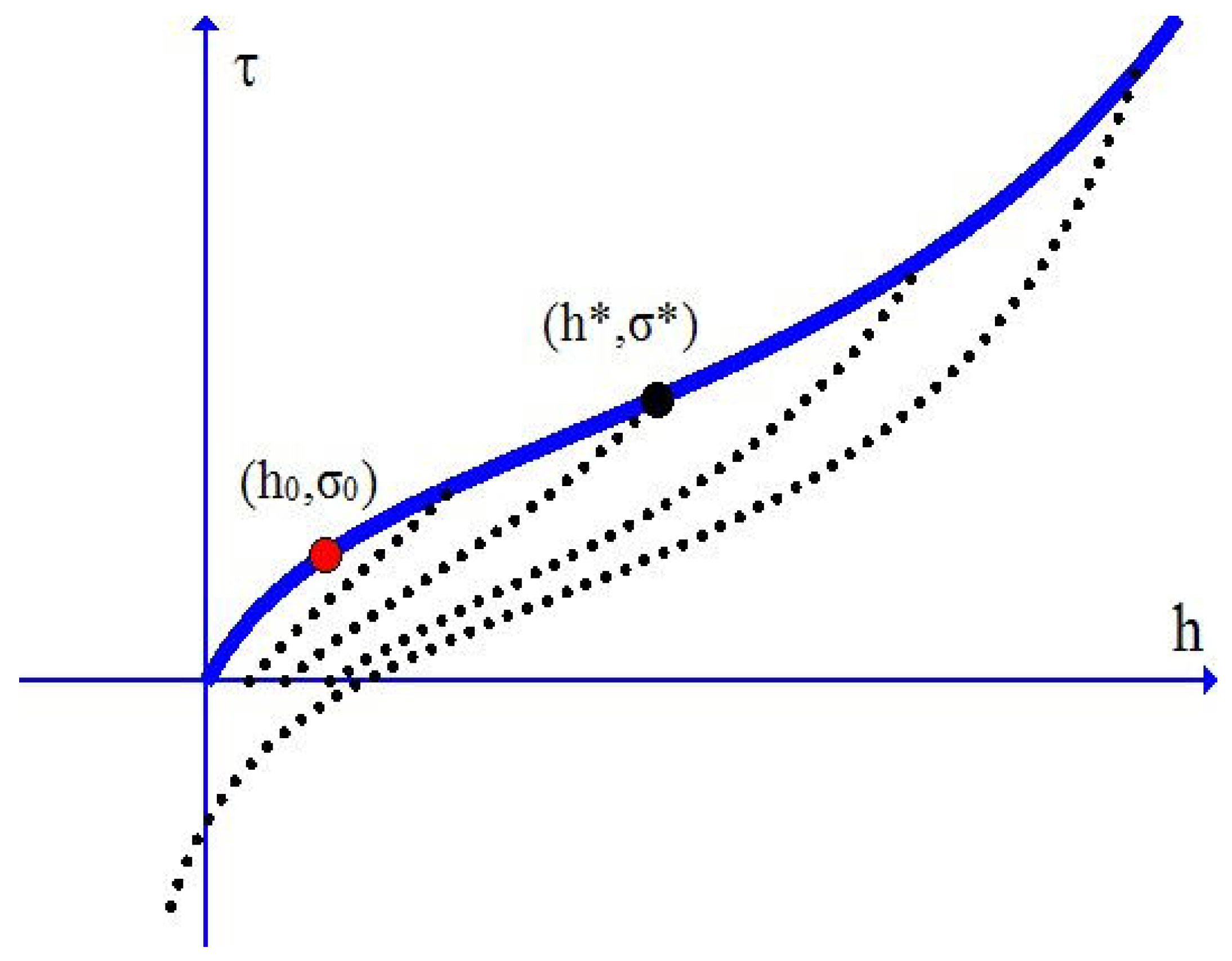
In this section, we first take the isothermal case into account. In this case, the temperature T is not involved. For a SMP sample, test data for uniaxial responses are given both for the monotone loading case and for various cases of unloading, as shown in Figure 1. For usual models with certain parameters to be identified, model predictions for given trial values of parameters should be compared with test data for the purpose of model validation. For a reasonable model, by means of trial-and-error procedures of searching for suitable forms of the constitutive functions and parameters, agreement with test data should be eventually achieved after iterative numerical procedures. Since both the loading curve and each unloading curve display complicated nonlinearities coupled with large strain and, in particular, a number of unloading curves should be taken into consideration and any two of them may be of different shapes, as shown in Figure 1, usual implicit procedures for both searching for reasonable forms of constitutive functions and identifying a set of unknown parameters would be unduly complicated.

We are going to demonstrate that, toward representing the stress-softening behavior of SMPs, explicit procedures may be introduced to obtain the three constitutive quantities in the proposed model, in such a sense that the model predictions can automatically, accurately fit any given sets of data both for the uniaxial monotone loading case and for various unloading cases.

3.1. Uniaxial Loading and Unloading Curves

Figure 1 shows the stress-softening effect at unloading, i.e., the well known Mullins effect. When a sample is loaded to a certain point $(h^{*},{\mathbf{\tau }}^{*})$ and then unloaded, there emerges the stress-softening effect as described below:

(i)

After the unloading is completed, a residual strain (permanent set) may be induced. The stress-strain curve in an unloading process may appreciably deviate from the monotone loading curve up to the unloading point $(h^{*},{\mathbf{\tau }}^{*})$ at the onset of unloading;

(ii)

for each strain $h\in [0,h^{*})$, the stress on the unloading curve is always lower than the stress on the monotone loading curve, referred to as stress softening at unloading;

(iii)

when reloading is introduced, the part of the reloading curve till the point $(h^{*},{\mathbf{\tau }}^{*})$ is nearly coincident with the unloading curve in the foregoing, but the part of the reloading curve after the point $(h^{*},{\mathbf{\tau }}^{*})$ follows the monotone loading curve after a transition at the point $(h^{*},{\mathbf{\tau }}^{*})$.

For a SMP sample of interest, test data are given for the loading curve and for a certain number of unloading curves. Consider M data sets for the unloading curves associated with M unloading stresses

$${\mathbf{\tau }}_1^{*}<{\mathbf{\tau }}_2^{*}<\cdots <{\mathbf{\tau }}_M^{*},$$

which correspond to M values of the effective plastic work below:

$${\tilde{\kappa }}_1<{\tilde{\kappa }}_2<\cdots <{\tilde{\kappa }}_M.$$

Specifically, for the unloading curve associated with the unloading stress ${\mathbf{\tau }}_s^{*}$ or the effective plastic work ${\kappa }_s$ for each $s\in \{0,1,\cdots ,M\}$, a set of strain-stress data is given below:

$$(h_0^{\left(s\right)},{\mathbf{\tau }}_0^{\left(s\right)}),(h_1^{\left(s\right)},{\mathbf{\tau }}_1^{\left(s\right)}),\cdots ,(h_{N_s}^{\left(s\right)},{\mathbf{\tau }}_{N_s}^{\left(s\right)}).$$

(12)

In the above, the first point $(h_0^{\left(s\right)},{\mathbf{\tau }}_0^{\left(s\right)})$ is just given by the strain $h_s^{*}$ and the stress ${\mathbf{\tau }}_s^{*}$ at the onset of unloading, and, moreover, the residual strain (permanent set) at vanishing stress, i.e., the point $(h_s^p,0)$, should be incorporated in the above set of data.

For any given data for the loading curve and any given sets of data for a certain number of unloading curves, as described in the above, it needs to find out such three quantities $\overline{W}$ (cf., Equation (3)) and r (cf., Equation (7)) and c (cf., Equation (9)) that the predictions from the model established in Section 2 fit these data as closely as possible. In what follows, we are going to show that explicit procedures may be introduced to obtain these constitutive quantities in a sense of accurately matching test data for any given shapes of loading and unloading curves.

3.2. The Evolving Elastic Potential

We first present the evolving elastic potential $\overline{W}$. The main procedures will follow those suggested in a previous study [40]. Details will be omitted below and may be referred to this reference.

A single-variable function for the unloading curve starting at the unloading point $(h_s^{*},{\mathbf{\tau }}_s^{*})$ may be obtained in a sense of accurately fitting any given date set as shown in Equation (12). Indeed, it may be given by an interpolating function, such as a Lagrange interpolant and an other form of function. Let such a function be designated by

$$h=g_s\left(\mathbf{\tau }\right)\mathrm{for}\mathrm{unloading}\mathrm{curves}s=1,\cdots ,M,$$

(13)

with

$$\left\{\begin{array}{c}{g}_s\left(0\right)=h_s^p,\hfill \\ g_s\left({\mathbf{\tau }}_{\mathit{\alpha }}\right)=h_{\mathit{\alpha }},\hfill \\ \mathit{\alpha }=0,1,\cdots ,N_s.\hfill \end{array}\right.$$

In the uniaxial case, it may readily be shown that the evolving potential Equation (2) reduces to a function of the axial Kirchhoff stress $\mathbf{\tau }$ and the effective plastic work $\tilde{\kappa }$, denoted

$$\begin{array}{c}\hfill \overline{w}=\overline{w}(\mathbf{\tau },\tilde{\kappa }).\end{array}$$

(14)

For the unloading curve starting at the unloading point $(h_s^{*},{\mathbf{\tau }}_s^{*})$, the elastic rate Equation (3) with $\dot{T}=0$ yields

$$\begin{array}{c}\hfill \dot{h}=\dot{\overline{\left(\frac{\partial \overline{w}}{\partial \mathbf{\tau }}\right)}}.\end{array}$$

For the unloading curve at issue, the effective plastic work is held fixed and given by ${\tilde{\kappa }}_s$. Then, the integration of this equation from the point $(h_s^p,0)$ to the point $(h,\mathbf{\tau })$ in an unloading process gives rise to

$$h-h_s^p=\frac{\mathit{D}{\overline{w}}_s}{\mathit{D}\mathbf{\tau }},$$

(15)

where ${\overline{w}}_s=\overline{w}(\mathbf{\tau },{\tilde{\kappa }}_s)$. In deriving Equation (15), the following initial condition is used:

$${\left.\frac{\partial \overline{w}}{\partial \mathbf{\tau }}\right|}_{\mathbf{\tau }=0}=0.$$

(16)

From Equation (15) and $h=g_s\left(\mathbf{\tau }\right)$ we deduce

$$\frac{\mathit{D}{\overline{w}}_s}{\mathit{D}\mathbf{\tau }}=g_s\left(\mathbf{\tau }\right)-h_s^p.$$

(17)

This produces

$${\overline{w}}_s={\overline{w}}_s\left(\mathbf{\tau }\right)={\int }_0^{\mathbf{\tau }}\left(g_s\left(\mathbf{\tau }\right)-h_s^p\right)\mathit{D}\mathbf{\tau }.$$

(18)

From the above procedures we obtain M uniaxial potentials ${\overline{w}}_1,\cdots ,{\overline{w}}_M$ for the M unloading curves at issue. However, each of them is restricted to the uniaxial case. The potential for general multiaxial deformations is obtainable from these uniaxial potentials by means of direct procedures. In fact, replacement of the axial Cauchy stress $\mathbf{\tau }$ in each potential $\overline{w}\left(\mathbf{\tau }\right)$ with the invariant $\mathsf{\phi }$ (cf., Equation (10)) multiplied by the mode invariant γ (cf., [49]) yields a multi-axial potential below:

$$\left\{\begin{array}{c}{\overline{W}}_s={\overline{w}}_s\left(\gamma \mathsf{\phi }\right),\hfill \\ \gamma =4.5tr{\tilde{\mathbf{\tau }}}^3/{\mathsf{\phi }}^3.\hfill \end{array}\right.$$

(19)

It may be verified that, in the uniaxial case, each function ${\overline{W}}_s$ for general multi-axial deformations, given by Equation (19), exactly supplies its uniaxial counterpart ${\overline{w}}_s$. We seek for a multi-axial potential $\overline{W}(\tilde{\mathbf{\tau }},\tilde{\kappa })$ which exactly gives the M multi-axial potentials ${\overline{W}}_1,\cdots ,{\overline{W}}_M$ for $\tilde{\kappa }={\tilde{\kappa }}_1,\cdots ,{\tilde{\kappa }}_M$. Such a potential may be given by an interpolating function with the M interpolating nodes $({\kappa }_s,{\overline{W}}_s)$ for $s=1,\cdots ,M$. For instance, it may be given by a Lagrange interpolant below:

$$\overline{W}=\overline{W}(\tilde{\mathbf{\tau }},\tilde{\kappa })=\sum _{s=1}^M{\overline{W}}_s{L}_s\left(\tilde{\kappa }\right)$$

(20)

with the Lagrangian base functions

$$L_s\left(\tilde{\kappa }\right)=\frac{P\left(\tilde{\kappa }\right)}{(\tilde{\kappa }-{\tilde{\kappa }}_s)P^{\prime }\left({\tilde{\kappa }}_s\right)},s=1,\cdots ,M,$$

(21)

$$P\left(\tilde{\kappa }\right)=\prod _{s=1}^M(\tilde{\kappa }-{\tilde{\kappa }}_s).$$

(22)

It may be a straightforward matter to show that, in the uniaxial case, the multi-axial potential Equation (20) exactly supplies the M uniaxial potentials ${\overline{w}}_1\left(\mathbf{\tau }\right),\cdots ,{\overline{w}}_M\left(\mathbf{\tau }\right)$ given by Equation (18) and, therefore, exactly fit any given M sets of data for M unloading curves (cf., Equation (13)).

With sufficient test data for a certain number of unloading curves, a single-variable function representing each unloading curve may be directly given either by an interpolating function or by choosing an other suitable form of function (see Section 4) .

3.3. Stress Limit and Prager Modulus

We next determine the stress limit r and the Prager modulus c. Let a set of data be given for a monotone stress-strain curve starting at the initial yield point $(h_0,{\mathbf{\tau }}_0)$ (cf., Figure 1). Then, a single-variable function representing this curve may also be directly given either by an interpolating function or an other form of function, as shown below:

$$\left\{\begin{array}{c}h=f\left(\mathbf{\tau }\right)\mathrm{for}\mathrm{the}\mathrm{loading}\mathrm{curve},\hfill \\ h_0=f\left({\mathbf{\tau }}_0\right),\mathbf{\tau }\ge {\mathbf{\tau }}_0,\hfill \end{array}\right.$$

(23)

For the monotone loading in the uniaxial case, from the $J_2$-flow model in Section 2 the four reduced equations below may be derived:

$$\mathbf{\tau }-\mathit{\alpha }=r,$$

$$\dot{h}=\dot{\overline{\left(\frac{\partial \overline{w}}{\partial \mathbf{\tau }}\right)}}+\frac{4}{9}{r}^2{\widehat{h}}^{-1}\dot{\mathbf{\tau }},$$

$$\dot{\tilde{\kappa }}=\frac{4}{9}{r}^3{\widehat{h}}^{-1}\dot{\mathbf{\tau }},$$

$$\widehat{h}=\frac{2}{3}c{r}^2+\frac{4}{9}{r}^3{r}^{\prime }.$$

In the above, $\overline{w}=\overline{w}(\mathbf{\tau },\tilde{\kappa })$ is the reduced form of the elastic potential Equation (20) in the uniaxial case and given by

$$\overline{w}=\sum _{s=1}^M{\overline{w}}_s\left(\mathbf{\tau }\right)L_s\left(\tilde{\kappa }\right),$$

(24)

where ${\overline{w}}_s\left(\mathbf{\tau }\right)$ and $L_s\left(\tilde{\kappa }\right)$ are given by Equations (18), (22) and (23).

In the monotone loading case, the axial stress $\mathbf{\tau }$ may be reformulated as a function of the effective plastic work $\tilde{\kappa }$, namely, $\mathbf{\tau }=q\left(\tilde{\kappa }\right).$ As such, from the last three of the foregoing four equations the following two equations may be derived:

$$\left\{\begin{array}{c}{\mathbf{\tau }}^{\prime }=r^{\prime }+1.5\frac{c}{r},\hfill \\ \frac{\mathit{D}}{\mathit{D}\tilde{\kappa }}\left(f\left(\mathbf{\tau }\right)-\frac{\partial \overline{w}}{\partial \mathbf{\tau }}\right)=\frac{1}{r},\hfill \end{array}\right.$$

(25)

The stress limit r may be given as follows [40,46,47,48]:

$$r=r_{\infty }+({\mathbf{\tau }}_0-r_{\infty })e^{-\mathsf{\beta }\tilde{\kappa }},$$

(26)

where $r_{\infty }>0$ is a constant and $\mathsf{\beta }>0$ is a large dimensionless parameter. For a large $\mathsf{\beta }>0$, the exponential function in Equation (26) rapidly goes to vanish for $\tilde{\kappa }>\mathsf{\delta }$ and the stress limit above is almost constant, i.e., $r\dot{}=r_{\infty }$ for $\tilde{\kappa }>\mathsf{\delta }$. Here $\mathsf{\delta }$ is very small. The localized property just mentioned means that, after the initial yielding, the stress limit r may be taken to be constant and given just by $r_{\infty }$, as will be done below.

By setting $r=r_{\infty }$, the integration of Equation (25)₂ from the initial yield point $(h_0,{\mathbf{\tau }}_0)$ to a point $(h,\mathbf{\tau })$ along the monotone curve in Figure 1 yields

$$\tilde{\kappa }=r_{\infty }\left(f\left(\mathbf{\tau }\right)-\frac{\partial \overline{w}}{\partial \mathbf{\tau }}\right).$$

(27)

At each unloading point $(h_s^{*},{\mathbf{\tau }}_s^{*})$, the derivative $\partial \overline{w}/\partial \mathbf{\tau }$ is just given by Equation (15) with $\mathbf{\tau }={\mathbf{\tau }}_s^{*}$. From this and Equation (17) and $f\left({\mathbf{\tau }}_s^{*}\right)=g_s\left({\mathbf{\tau }}_s^{*}\right)$ we obtain the effective plastic works at the M unloading points as follows:

$${\tilde{\kappa }}_s=r_{\infty }{h}_s^p,s=1,2,\cdots ,M,$$

(28)

where $h_s^p$ and ${\tilde{\kappa }}_s$ are the plastic strain and the effective plastic work associated with the s-th unloading curve.

Next, Equation (25)₂ with $r=r_{\infty }$ may be converted to

$$\left(\frac{\mathit{D}f}{\mathit{D}\mathbf{\tau }}-\frac{{\partial }^2\overline{w}}{\partial {\mathbf{\tau }}^2}\right){\mathbf{\tau }}^{\prime }=\frac{{\partial }^2\overline{w}}{\partial \mathbf{\tau }\partial \tilde{\kappa }}+\frac{1}{r_{\infty }}.$$

(29)

From this and Equation (25)₁, an expression for the Prager modulus c in the uniaxial case may be obtained in terms of the axial stress $\mathbf{\tau }$ and the $\tilde{\kappa }$. Replacing $\mathbf{\tau }$ by the invariant $\mathsf{\phi }$ in Equation (19) we eventually obtain Prager’s modulus for general multi-axial cases as follows:

$$c=\frac{2}{3}\frac{1+r_{\infty }\mathsf{\varphi }(\mathsf{\phi },\tilde{\kappa })}{f^{\prime }\left(\mathsf{\phi }\right)-\mathsf{\zeta }(\mathsf{\phi },\tilde{\kappa })},$$

(30)

where

$$\left\{\begin{array}{c}\mathsf{\varphi }(\mathbf{\tau },\tilde{\kappa })=\frac{{\partial }^2\overline{w}}{\partial \mathbf{\tau }\partial \tilde{\kappa }}=\sum _{s=1}^M\left(g_s\left(\mathbf{\tau }\right)-h_s^p\right)L_s^{\prime }\left(\tilde{\kappa }\right),\hfill \\ \mathsf{\zeta }(\mathbf{\tau },\tilde{\kappa })=\frac{{\partial }^2\overline{w}}{\partial {\mathbf{\tau }}^2}=\sum _{s=1}^M{g_s}^{\prime }\left(\mathbf{\tau }\right)L_s\left(\tilde{\kappa }\right),\hfill \end{array}\right.$$

(31)

where $L_s\left(\tilde{\kappa }\right)$ is given by Equations (22) and (23).

4. Shape Functions for Uniaxial Loading and Unloading Curves

With the evolving elastic potential $\overline{W}$, the stress limit r and the Prager modulus c given in the last section, the elastoplastic $J_2$-flow model established in Section 2 exactly reproduces the monotone loading curve $h=f\left(\mathbf{\tau }\right)$ and any given number of unloading curves, $h=g_s\left(\mathbf{\tau }\right)$. It may be straightforward to find out suitable forms of such single-variable functions fitting any given data for the monotone loading case and for various unloading cases, without involving usual complicated procedures of treating several nonlinear differential equations incorporating a number of parameters to be identified. The foregoing two kinds of single-variable functions, referred to as the shape functions for loading und unloading curves, may be given directly by usual interpolating functions fitting any given data without error. Alternatively, these shape functions may also be given by other forms of functions. In particular, it is of interest to have simple forms of shape functions with parameters of direct physical meanings. Such forms of shape functions are given below.

Firstly, below a simple form of the shape function is given to represent each unloading curve:

$$\mathbf{\tau }=\frac{(1-\mathsf{\gamma })E(h-h^p)}{1-\frac{h-h^p}{u}}+\mathsf{\gamma }E(h-h^p)\mathrm{for}h-h^p\ge 0,$$

(32)

and its inverted form is as follows:

$$\begin{array}{c}\hfill h=g\left(\mathbf{\tau }\right)=h^p+\frac{2u\sigma }{\mathbf{\tau }+Eu+\sqrt{{(\mathbf{\tau }+Eu)}^2-4{\mathsf{\gamma }}^{+}Eu\sigma }}.\end{array}$$

(33)

In the above, $h^p$ is the plastic strain after unloading, E is the Young’s modulus at infinitesimal strain, u is the strain limit and $\mathsf{\gamma }<1$ is dimensionless parameter characterizing the growth degree of stress as the strain is approaching the strain limit u. In general, each of these parameters may rely on the effective plastic work $\tilde{\kappa }$, namely,

$$\begin{array}{c}\hfill E=E\left(\tilde{\kappa }\right),u=u\left(\tilde{\kappa }\right),\mathsf{\gamma }=\mathsf{\gamma }\left(\tilde{\kappa }\right).\end{array}$$

(34)

For each unloading curve associated with a value of the effective plastic work, values of the above parameters may be determined by fitting the above shape function to given data. As such, a set of parameter values may be obtained for a family of unloading curves. Then, each of the foregoing $\tilde{\kappa }$-dependent parameter may also be given directly by an interpolating function. It may be noted that the parameters introduced directly represent the very features of each elastic unloading curve at issue and, accordingly, are determinable from each unloading curve in a decoupled manner.

In particular, the unloading curve starting at the initial yield points $(h_0,{\mathbf{\tau }}_0)$ is associated with $\tilde{\kappa }=0$ and coincident exactly with the initial elastic curve from the origin to the initial yield point (cf., Figure 1). This curve may be given simply by a linear relation between the axial stress $\mathbf{\tau }$ and the axial Hencky strain h, namely,

$$\left\{\begin{array}{c}h=g_0\left(\mathbf{\tau }\right)=\frac{\mathbf{\tau }}{E_0}(0\le \mathbf{\tau }\le {\mathbf{\tau }}_0),\hfill \\ \tilde{\kappa }=0,\hfill \end{array}\right.$$

(35)

where $E_0=E\left(0\right)$ is the initial Young’s modulus.

On the other hand, the shape function for the monotone loading curve starting at the initial yield points $(h_0,{\mathbf{\tau }}_0)$ may be given by (c.f., [46,47,48])

$$\begin{array}{c}\hfill \left\{\begin{array}{cc}h\hfill & =f\left(\mathbf{\tau }\right)=\frac{{\mathbf{\tau }}_0}{E}+{\mathsf{\xi }}_0(\mathbf{\tau }-{\mathbf{\tau }}_0)+\hfill \\ & +\frac{1}{2}({\mathsf{\xi }}_1(\mathbf{\tau }-{\mathbf{\tau }}_0-s)+a_0)\left(tanh\left(m(\mathbf{\tau }-{\mathbf{\tau }}_0-s)\right)+tanh\left(ms\right)\right).\hfill \end{array}\right.\end{array}$$

(36)

The meanings of the parameters incorporated may be found in previous works [46,47,48].

The above shape functions for the monotone loading curve and the unloading curves of SMPs are new and much simpler, as compared with the counterparts in a most recent study [40]. With these new shape functions, accurate accord with test data may be achieved, as will be shown in Section 6.1.

5. Large Strain Recovery Effect at Heating

In this section, large strain recovery effect in a thermo-mechanical process consisting of an isothermal loading-unloading process and then a heating process will be derived from the proposed model. It will be shown that the proposed model predicts a pre-strain induced in the isothermal loading -unloading process and then a plastic flow induced in the heating process. It will further be shown that such thermo-induced plastic flow may be responsible for the recovery of the pre-strain induced in the isothermal loading-unloading process. This represents the very feature of the shape memory effect of SMPs. It will also be shown that, from the proposed model, simple and exact results may be derived for a general multiaxial case.

5.1. Pre-Strain Induced at Isothermal Loading-Unloading

We first consider an isothermal loading-unloading process. Let the temperature be held fixed and given by $T_0$. In this case, a polymer sample is monotonically loaded to a certain stress level and then unloaded to zero stress. The stress and strain responses at both loading and unloading may be determined from the proposed model with the isothermal constitutive quantities obtained in Section 3. For the uniaxial case, in particular, the response at loading is given by Equation (23) and the response at unloading by one of those in Equation (13).

After unloading at temperature $T_0$, a pre-strain or permanent set, denoted $h_0$, is induced, namely,

$$\begin{array}{c}\hfill \left\{\begin{array}{c}{\mathit{h}}_0=\frac{1}{2}ln\left({\mathit{F}}_0{\mathit{F}}_0^T\right),\hfill \\ {\mathit{F}}_0{=\mathit{F}|}_{T=T_0},\hfill \end{array}\right.\end{array}$$

(37)

and, besides, the effective plastic work and the back stress are designated by ${\tilde{\kappa }}_0$ and ${\mathit{\alpha }}_0$, viz.,

$$\begin{array}{c}\hfill \tilde{\kappa }{{|}_{T=T_0}={\tilde{\kappa }}_0,\mathit{\alpha }|}_{T=T_0}={\mathit{\alpha }}_0.\end{array}$$

(38)

Note here that a general multi-axial case is taken into account.

5.2. Thermo-Induced Plastic Flow at Heating

We next treat a process of pure heating with the temperature T changing from $T_0$ to $T_{*}$. In this case, the stress limit r relies merely on the temperature T. Usually, r should decrease with increasing temperature. Namely,

$$r^{\prime }\left(T\right)=\frac{\mathit{D}r}{\mathit{D}T}<0.$$

(39)

With an initial temperature $T_0$ held fixed, a pre-strain or plastic strain is induced in a SMP sample via a loading-unloading process at constant temperature $T_0$, as indicated in Section 5.1. Let

$$f\left(T\right)=\frac{1}{2}{\left|{\mathit{\alpha }}_0\right|}^2-\frac{1}{3}{\left(r\left(T\right)\right)}^2.$$

(40)

The unloading at $T=T_0$ leads to

$$f\left(T_0\right)=\frac{1}{2}{\left|{\mathit{\alpha }}_0\right|}^2-\frac{1}{3}{\left(r\left(T_0\right)\right)}^2<0.$$

(41)

Consider a heating process with $\dot{T}>0$. On account of Equation (39), the $f\left(T\right)$ increases with increasing temperature and hence it may increase from the initial value $f\left(T_0\right)<0$ at $T_0$ to zero at a certain temperature $T_0^{*}$, namely,

$$f\left(T_0^{*}\right)=\frac{1}{2}{\left|{\mathit{\alpha }}_0\right|}^2-\frac{1}{3}{\left(r\left(T_0^{*}\right)\right)}^2=0.$$

(42)

Moreover, with $\tilde{\mathbf{\tau }}=O$ and $\dot{T}>0$ as well as Equation (40) we deduce that

$$\frac{1}{\widehat{h}}\left(\frac{\partial f}{\partial \tilde{\mathbf{\tau }}}:\stackrel{\mathrm{o}}{\tilde{\mathbf{\tau }}}{}^{\log }+\frac{\partial f}{\partial T}\dot{T}\right)=-{\left(cr\right)}^{-1}{r}^{\prime }\left(T\right)\dot{T}>0.$$

(43)

Hence, from Equation (8)₁ it follows that the loading condition is met. Thus, plastic flow may be induced at pure heating and emerges for $T\ge T_0^{*}$.

By setting $\mathbf{\tau }=O$ in the rate equations given in Section 2, the governing equations for the thermo-induced plastic flow as indicated above may be derived as follows:

$$\mathit{D}={\mathit{D}}^e+{\mathit{D}}^p,$$

(44)

$${\mathit{D}}^e={\mathsf{\Theta }}^{\prime }\left(T\right)\dot{T}\mathit{I},$$

(45)

$${\mathit{D}}^p=r^{\prime }\left(T\right)\frac{\dot{T}}{cr}\mathit{\alpha },$$

(46)

$$\stackrel{\mathrm{o}}{\mathit{\alpha }}{}^{log}=\frac{1}{r}{f}^{\prime }\left(T\right)\dot{T}\mathit{\alpha },$$

(47)

$$\dot{\tilde{\kappa }}=\frac{2}{3}{c}^{-1}r{r}^{\prime }\left(T\right)\dot{T},$$

(48)

with the initial conditions at $T=T_0^{*}$ given below:

$$\begin{array}{c}\hfill \left\{\begin{array}{c}{\mathit{F}|}_{T=T_0^{*}}=e^{{\mathsf{\Theta }}_0^{*}-{\mathsf{\Theta }}_0}{\mathit{F}}_0,{\mathsf{\Theta }}_0^{*}=\mathsf{\Theta }\left(T_0^{*}\right),{\mathsf{\Theta }}_0=\mathsf{\Theta }\left(T_0\right),\hfill \\ {\mathit{\alpha }|}_{T=T_0^{*}}={\mathit{\alpha }}_0,\tilde{\kappa }{|}_{T=T_0^{*}}={\tilde{\kappa }}_0{,r|}_{T=T_0^{*}}=\sqrt{1.5}\left|{\mathit{\alpha }}_0\right|.\hfill \end{array}\right.\end{array}$$

(49)

In deriving Equation (49), the following fact has been used: only thermo-elastic volumetric deformation is induced from $T_0$ to $T_0^{*}$.

A closed-form solution may be derived from the above equations. Results are as follows:

$$\mathit{\alpha }=\sqrt{\frac{2}{3}}\frac{{\mathit{\alpha }}_0}{|{\mathit{\alpha }}_0|}r\left(T\right),T\ge T_0^{*},$$

(50)

for the back stress, and

$$\begin{array}{c}\hfill \left\{\begin{array}{c}\mathit{F}=e^{\mathsf{\Theta }-{\mathsf{\Theta }}_0}{\mathit{F}}_0,\hfill \\ \mathit{h}=\left(\mathsf{\Theta }-{\mathsf{\Theta }}_0\right)\mathit{I}+{\mathit{h}}_0+\sqrt{\frac{2}{3}}\frac{{\mathit{\alpha }}_0}{|{\mathit{\alpha }}_0|}{\int }_{T_0^{*}}^T{c}^{-1}{r}^{\prime }\left(T\right)\mathit{D}T,T\ge T_0^{*},\hfill \end{array}\right.\end{array}$$

(51)

for the deformation gradient and Hencky’s logarithmic strain, and, finally,

$$\tilde{\kappa }={\tilde{\kappa }}_0+\frac{2}{3}{\int }_{T_0^{*}}^T{c}^{-1}r{r}^{\prime }\left(T\right)\mathit{D}T,T\ge T_0^{*},$$

(52)

for the effective plastic work.

5.3. Strain Recovery Effect

Equation (51) supplies a closed-form solution for the Hencky strain in a thermo-mechanical process consisting of an isothermal loading-unloading process at constant temperature $T_0$ and then a pure heating process from $T_0$ to a higher temperature T, in which a thermo-induced plastic flow is induced from $T_0^{*}$ to T. This result has been derived for a general multi-axial case. The Hencky strain given is composed of three parts, namely, the pre-strain $h_0$ at $T_0$, the thermo-elastic volumetric strain $(\mathsf{\Theta }-{\mathsf{\Theta }}_0)\mathit{I}$, as well as the part from the thermo-induced plastic flow. The thermo-elastic expansion part is usually very small, but it may become appreciable in a process through the glass transition in some cases. Generally, the thermo-elastic expansion effect over a temperature range may be simulated by choosing a suitable form of the temperature-dependent quantity $\mathsf{\Theta }\left(T\right)$.

With negligible thermo-elastic expansion, it may be demonstrated [40] that the minimum of the magnitude of the strain $h$ as given in Equation (51) is always smaller than the initial value $|h_0|$ at $T_0$. This suggests that generally the thermo-induced plastic flow in a process of pure heating always leads to a partial recovery of any given pre-strain. As such, the thermal recovery at pure heating is derived as a direct, natural consequence of the thermo-coupled elastoplasticity model established in Section 2. In particular, it may be deduced that the complete recovery of any given pre-strain emerges whenever

$${\mathit{\alpha }}_0=c_0{\mathit{h}}_0$$

(53)

with the $c_0$ a constant. In particular, the above co-axiality condition is identically fulfilled in the uniaxial strain case.

Now, the Prager modulus c is taken to be of the following form [40]:

$$c=\frac{1}{2}(c_0+c_0^{*})-\frac{1}{2}(c_0-c_0^{*})tanh\left[\mathsf{\lambda }\frac{T-T_0}{T_0^{*}-T_0}\right].$$

In the above, $c_0^{*}<c_0$ and $\mathsf{\lambda }>0$ is a large dimensionless parameter. Then, the Hencky strain for $T\ge T_0^{*}$ is given by (c.f., [40])

$$\begin{array}{c}\hfill \left\{\begin{array}{c}\mathit{h}=\left(\frac{c_0}{c_0^{*}}\frac{r}{r_0^{*}}-\frac{c_0}{c_0^{*}}+1\right){\mathit{h}}_0,\hfill \\ r_0^{*}{=r|}_{T=T_0^{*}}=\sqrt{1.5}{c}_0\left|{\mathit{h}}_0\right|.\hfill \end{array}\right.\end{array}$$

(54)

This result applies to a general multiaxial case. Given any form of the uniaxial temperature-strain relation, $h=h\left(T\right)$, the temperature-dependent stress limit r is thus determined, as shown below:

$$r=c_0^{*}\left[h\left(T\right)-h_0\right]+c_0{h}_0.$$

(55)

With the above stress limit, the proposed model exactly reproduces the strain-temperature relation $h=h\left(T\right)$ and, accordingly, any given uniaxial data for strain recovery may be automatically, accurately fitted.

An example for the stress limit r with strain recovery is given as follows:

$$\begin{array}{c}\hfill r=r_0^{*}\left[1-\frac{c_0^{*}}{c_0}tanh\mathsf{\lambda }\frac{T-T_0^{*}}{T_m-T_0^{*}}\right],\end{array}$$

(56)

where both the temperature $T_0^{*}>T_0$ at the initial yielding (cf. Equation (42)) and the temperature $T_m>T_0^{*}$ may be of any given values. The corresponding strain-temperature function is given by

$$\begin{array}{c}\hfill h=h_0\left[1-tanh\mathsf{\lambda }\frac{T-T_0^{*}}{T_m-T_0^{*}}\right].\end{array}$$

(57)

For a fairly large $\mathsf{\lambda }$, any given large pre-strain, $h_0$, is almost completely recovered at a temperature slightly higher than $T_m$, as will be seen in the numerical example in the next section.

6. Numerical Examples

According to the results derived in the preceding sections, the predictions from the proposed model may automatically, accurately fit any given data for both the stress-softening effect and the strain recovery effect simply by choosing three shape functions $h=f\left(\mathbf{\tau }\right)$, $h=g_s\left(\mathbf{\tau }\right)$, $h=h\left(T\right)$ that accurately fit these data. As indicated before, it may be straightforward to present these three shape functions by choosing usual interpolating functions. However, they may be given by other forms of functions. As illustrative examples, in this section the simple forms of shape functions given in Section 4 and Section 5.2 will be used to fit test data in literature.

In what follows, test data will be fitted by using the shape function Equation (36) for the initial elastic curve, the shape function (37) for the monotone loading curve and the shape function (34) for the unloading curve, as well as the strain-temperature function Equation (57) for the strain recovery curve.

Below, the model predictions will be compared with two sets of data in literature, separately.

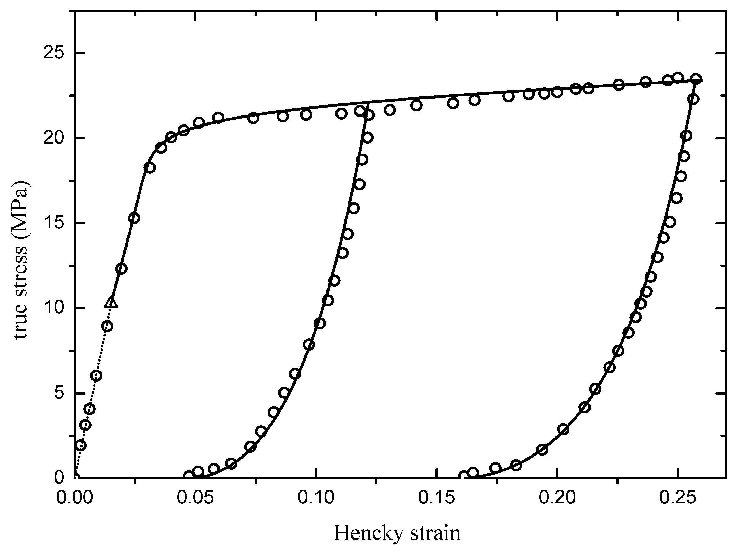
6.1. Data for Stress-Softening Effect at Unloading

We first consider the data from [27]. These data (Figure 8) are concerned with a SMP resin sample for the monotone loading case till the strain 23% and then for two unloading cases starting at two strains of 11% and 23%, separately.

The initial elastic curve is given by Equation (36) with

$$h_0=0.015,{\mathbf{\tau }}_0=10.30\mathrm{MPa},E_0=686.67\mathrm{MPa}.$$

The shape function for the monotone loading curve is given by Equation (37) with the parameter values below:

$${\mathbf{\tau }}_0=10.30\mathrm{MPa},E=680\mathrm{MPa},{\mathsf{\xi }}_0=0.001852{\mathrm{MPa}}^{-1},$$

$${\mathsf{\xi }}_1=0.067568{\mathrm{MPa}}^{-1},s=12.5\mathrm{MPa},m=0.5,a_0=0.3.$$

The two unloading curves are fitted by the shape function Equation (34) with

$$h_p=0.0475,u=0.154,E=5.782\mathrm{MPa},\mathsf{\gamma }=-53.179,$$

for the first unloading curve, and

$$h_p=0.162,u=0.167,E=12.361\mathrm{MPa},\mathsf{\gamma }=-13.218,$$

for the second unloading curve. Results are shown in Figure 2 by plotting the curves of the axial true stress against the axial Hencky strain. Good agreement with the given data is achieved.

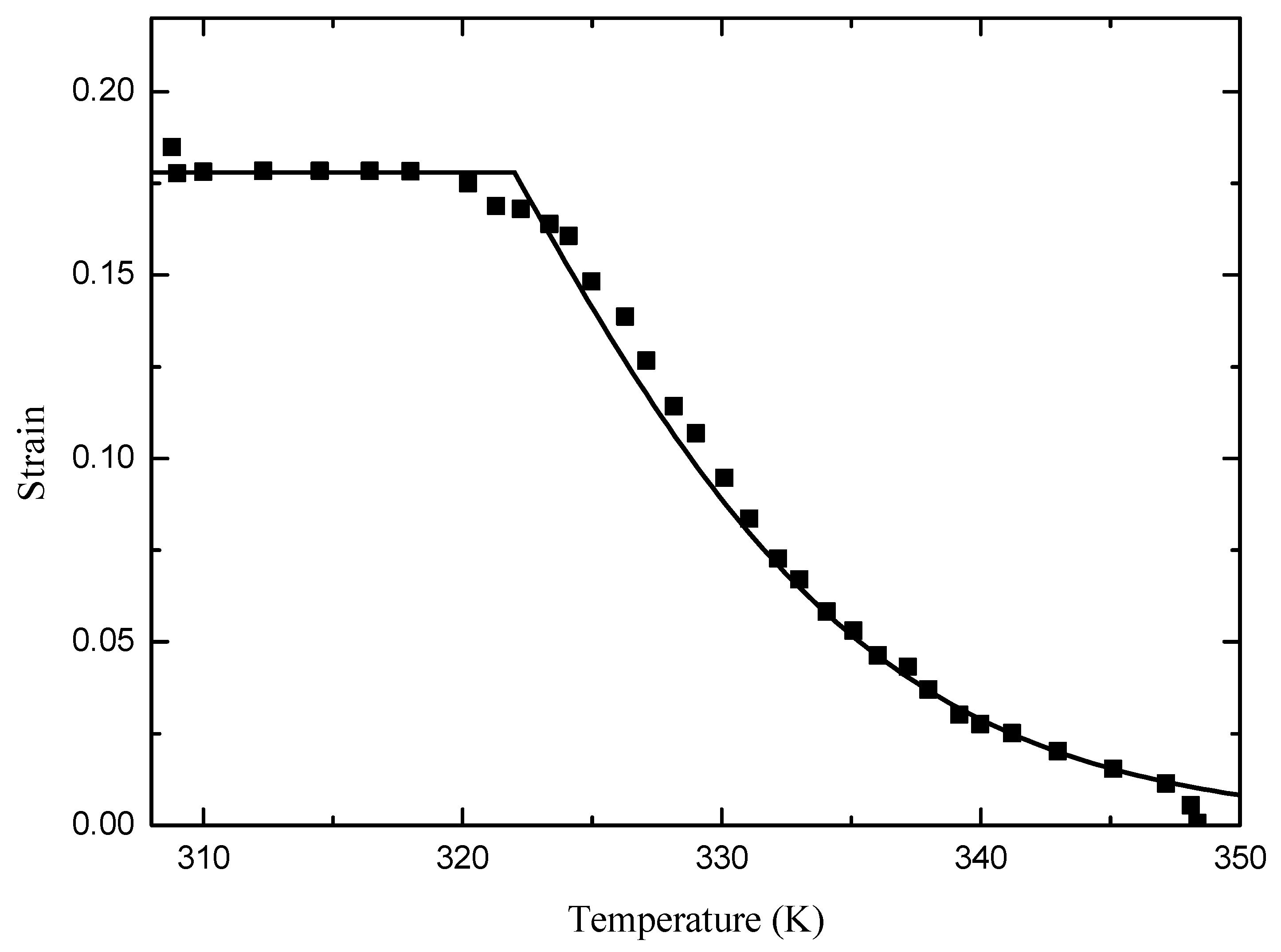
6.2. Data for Strain Recovery Effect at Heating

We next consider the data from [26] (Figure 5c), which are concerned with the strain recovery effect of a SMP sample in a heating process from 320 K to 350 K with the pre-strain 0.164.

The strain-temperature function Equation (57) is used to fit the data at issue, with the parameter values below:

$$h_0=0.164,\mathsf{\lambda }=1.7,T_0^{*}=322\mathrm{K},T_m=348\mathrm{K}.$$

Results are shown in Figure 3 by plotting the curve of the temperature against the axial Hencky strain. Again, good agreement with the given data is achieved.

7. Concluding Remarks

In the preceding sections, a new thermo-coupled elastoplastic $J_2$-flow models with evolving elastic behavior has been proposed to achieve an explicit, direct simulation of complicated inelastic behavior of SMPs displaying both the stress softening effect at unloading and the strain recovery effect at heating. The constitutive quantities incorporated in the proposed model are explicitly determined from suitable uniaxial data. Extensive test data for any given shapes of loading and unloading curves as well as the strain-temperature curve may be accurately, automatically fitted by means of single-variable shape functions. It has been demonstrated that all may be done in the scope of classical elastoplasticity and, therefore, that no additional variables need be introduced and treated. Usual implicit, complicated procedures both in searching for suitable forms of constitutive functions and in identifying values of unknown parameters may be bypassed.

This study represents a development of the model suggested in a most recent study [40]. Results in this reference are derived for certain usual deformation features of polymeric materials. However, new treatments need further be introduced for the purpose of simulating thermo-mechanical deformation features unique to SMPs. In fact, SMPs exhibit thermal effects and loading-unloading response features that differ in nature from those for usual polymers. As a consequence, the shape functions representing the loading curve and each unloading curve (cf., Figure 1) need be given in other suitable forms and, moreover, both thermal expansion and strain recovery need be considered in a unified manner. Here, new forms of shape functions that apply to deformation features of SMPs are presented in Section 4 and closed-form results with both thermal expansion and strain recovery effects are derived in Section 5. Good agreement with test data is achieved.

It should be pointed out that thermo-mechanical deformation features of SMPs may be simulated from various standpoints, as mentioned in the introduction section. Various constitutive models may be established based on additional variables associated with micro-structural mechanisms. Representatives are those based on either transition between micro-structural phases or evolution of macromolecular networks. For instance, transition between an active and a frozen phase is considered in [32] with a volume-fraction variable for the frozen phase, while evolution of a reversible and a permanent network is treated in [36,37,38]. It may be noted that the volume-fraction variable has been fruitfully used in modeling thermo-mechanical behavior of SMAs with the martensite-to-austenite phase transition mechanism. On the other side, various types of networks are directly related to certain aspects of cross-links and entanglements of chain-like macromolecules in polymeric materials.

Irrespective of the fact that the proposed model is straightforward in a sense without assuming any ad hoc variables of micro-structural origins, it may be of significance to explain how it accommodates itself to relevant underlying micro-mechanisms. For instance, the back stress $\mathit{\alpha }$, which plays an essential role in deriving the thermo-induced plastic flow responsible for the strain recovery effect in Section 5, may be explained based on the notion of a permanent network as introduced in [36,37,38]. In general, each macroscopic constitutive quantity introduced in the proposed model may be related to relevant micro-mechanisms via suitable averaged procedures. This respect need be studied in future.

It is known that thermo-mechanical responses of SMPs depend on both strain rate and thermo-mechanical history. For example, the loading curve and each unloading curve as shown in Figure 1 will be changed by strain rate and cyclic loading. In particular, cyclic thermo-mechanical loadings may lead to fatigue failure. Rate effects may be incorporated by introducing a rate-dependent stress limit in extending the proposed model. Furthermore, fatigue failure behavior may be simulated by extending the plastic flow Equation (5) to a new, free plastic flow equation without involving the usual loading-unloading conditions as stipulated in Equation (8). These may be done by a development of the most recent study [50,51]. Results will be reported elsewhere.

It should be noted that the anisotropy effect induced by plastic strain may be simulated by the proposed model with evolution of the back stress. For a SMP with initial anisotropy, such as a SMP composite with preferred directions, the thermo-elastic potential $\overline{W}(\tilde{\mathbf{\tau }},\tilde{\kappa },T)$ in Equation (2) should be restricted by the form-invariance requirements relative to a symmetry group representing the initial material symmetry. Detail may be found in [43].