Guided Self-Accelerating Airy Beams—A Mini-Review

Abstract

Owing to their nondiffracting, self-accelerating, and self-healing properties, Airy beams of different nature have become a subject of immense interest in the past decade. Their interesting properties have opened doors to many diverse applications. Consequently, the questions of how to properly design the spatial manipulation of Airy beams or how to implement them in different setups have become important and timely in the development of various optical devices. Here, based on our previous work, we present a short review on the spatial control of Airy beams, including the interactions of Airy beams in nonlinear media, beam propagation in harmonic potential, and the dynamics of abruptly autofocusing Airy beams in the presence of a dynamic linear potential. We demonstrate that, under the guidance of nonlinearity and an external potential, the trajectory, acceleration, structure, and even the basic properties of Airy beams can be adjusted to suit specific needs. We describe other fascinating phenomena observed with Airy beams, such as self-Fourier transformation, periodic inversion of Airy beams, and the appearance of spatial solitons in the presence of nonlinearity. These results have promoted the development of Airy beams, and have been utilized in various applications, including particle manipulation, self-trapping, and electronic matter waves.

1. Introduction

Diffraction is a fundamental phenomenon in physical optics, due to which beams bend and spread, and the peak intensity of the beam decreases upon propagation. Sometimes it is beneficial, as in the diffraction gratings, sometimes a nuisance, as in the diffraction limit. In situations where diffraction is not desired and needs to be overcome, the nondiffracting beams come to the fore. These beams are a class of nondispersive solutions of the Helmholtz wave equation that display exotic characteristics: they are nondiffracting, self-accelerating, and self-healing, among other properties. The representative nondiffracting beams include the radially symmetric Bessel beams and the asymmetric Airy beams.

In comparison with the Bessel beam, the most remarkable feature of an Airy beam is the self-acceleration in free space [1,2,3]. The Airy beam concept originated from quantum mechanics. In 1979, Berry and Balazs demonstrated that the Airy function is an eigenmode of the linear Schrödinger equation [1] and that it is the only nontrivial solution that does not expand with time and it accelerates in space. The paraxial wave equation—the wave equation in the paraxial approximation—has the same form as the linear Schrödinger equation. Based on this mathematical similarity between optics and quantum mechanics, one can get not only Airy beams and Airy pulses, but also other types of waves which satisfy the paraxial wave equation, such as surface plasmon polaritons [4,5], acoustic waves [6] and water waves [7,8], among others. Notably, the nondiffracting feature of an Airy beam comes from its infinite transverse extension and power, since the ideal Airy function is not square integrable. This feature is similar to the simple plane wave. Hence, to possess finite energy and become a physical quantity, the Airy beam must be truncated. In optics, this is simply achieved by an exponential aperture, as first put forward in 2007, by Siviloglou et al. [2,9]. The truncated Airy beam can still propagate for a long distance, preserving major characteristics of an ideal Airy beam, but eventually it will diffract and lose its unique structure and properties. Nonetheless, this method of generation makes the Airy beam experimentally available and of wide interest for applications in optical beam manipulation. However, this method also limits the light energy utilization and the stability of beams in the nonlinear domain. Still, by exploiting these unique characteristics of Airy beams, various application possibilities have been explored or implemented, for example, for Airy plasma guiding [10], routing surface plasmon polaritons [11], image signal transmission [12,13], laser filamentation [14], optical micromanipulation [15,16], optical trapping [17,18,19,20], light bullet generation [21,22,23,24], electron acceleration [25], and other applications [25,26,27,28,29].

In addition to research on Airy beams in free space and linear media, work has also been extended to nonlinear (NL) media and regimes. In the most common optical NL media, i.e., the Kerr, saturable and quadratic media, the nonlinearity is spatially modulated, so that the beam diffraction can be effectively balanced by the nonlinearity through a soliton-like beam generation process. In 2009, Ellenbogen et al. produced an Airy beam in an asymmetrically modulated quadratic optical NL medium by the three-wave mixing process [30]. This novel nonlinear generation method not only produced an Airy beam at a new wavelength and a higher energy, but also provided new possibilities for manipulating the dynamics of Airy beams in NL media [31,32,33,34,35]. According to the nonlinear Schrödinger equation, the nonlinearity plays a nontrivial role in controlling the persistence as well as the breakdown of Airy beams [36,37,38]. It has been demonstrated that the main lobe of an Airy beam experiences self-phase modulation in NL media that results in the self-focusing or trapping of the beam [33]. And the field distribution of the Airy beam varies differently in different NL media [36,39].

As is well known, the beam focusing is an efficient way to improve laser power density. Thanks to the self-accelerating feature of Airy beams, in 2010, Efremidis and Christodoulides proposed a novel abruptly autofocusing (AAF) beam [40]. The beam possesses a ring-shaped initial transverse Airy amplitude pattern, and accelerates in either the inward or outward direction, determined by the Airy wave function tail [41]. During propagation, the AAF beam can keep a low intensity profile initially, and then abruptly converge to a focal point where the intensity grows by orders of magnitude [40,42,43,44,45,46]. This abruptly autofocusing property of an AAF beam avoids the possible interaction of the beam with the transmission medium before focusing. It can be used in biomedical treatments, bottle beams, light bullets, and in other nonlinear settings.

To date, immense research work has been devoted to Airy beams, from theoretical predications to experimental verifications, from fundamental research to potential applications. Without doubt, it has become one of the hottest developing fields in linear and nonlinear optics [47,48,49,50]. In this short review, based on our previously published work, we discuss some robust and flexible manipulation techniques applied to Airy beams. The organization of the paper is as follows. Section 2 provides results and discussion. In Section 2.1, we describe the interaction of two Airy beams as they propagate simultaneously in a NL medium; in Section 2.2, we summarize Airy beam propagation in a harmonic potential; in Section 2.3, we discuss the controllable spatial modulation of AAF beams, under an action of different dynamic linear potentials. In Section 3, we conclude the paper.

2. Results and Discussion

In quantum mechanics, the Schrödinger equation (SE) for a quantum particle moving in free space is written as:

$$i\hslash \frac{\partial \psi }{\partial t}+\frac{{\hslash }^2}{2m}\frac{{\partial }^2\psi }{\partial x^2}=0,$$

(1)

where ℏ is the reduced Planck’s constant and m is the particle mass. This equation describes the development of the wave function $\psi$ of the particle, but in appropriate units it could also describe the development of an Airy wave packet.

In optics, the propagation of a scalar wave packet obeys the Helmholtz equation:

$$\left(\frac{{\partial }^2}{\partial x^2}+\frac{{\partial }^2}{\partial z^2}\right)\psi +k^2\psi =0,$$

(2)

where x and z are the transverse and longitudinal coordinates, and $k=2\pi n/{\lambda }_0$ is the wavenumber (n is the index of refraction and ${\lambda }_0$ the wavelength in free space). Under the paraxial approximation $|{\partial }_z^2\psi |\ll |2k{\partial }_z\psi |$, one obtains the paraxial wave equation,

$$i\frac{\partial \psi }{\partial z}+\frac{1}{2}\frac{{\partial }^2\psi }{\partial x^2}=0,$$

(3)

where now the variables x and z are the normalized transverse coordinate and the propagation distance, scaled by some characteristic transverse width $x_0$ and the corresponding Rayleigh range $k{x}_0^2$. Obviously, Equation (3) has the same form as Equation (1) in scaled units—it is just the SE without potential—so one of the accelerating solutions of Equation (3) is the well-known Airy function with the characteristic infinite oscillatory tail,

$$\psi (x,z)=\mathrm{Ai}\left(x-\frac{z^2}{4}\right)\exp \left[\frac{i}{12}\left(6xz-z^3\right)\right].$$

(4)

From this solution, it is not hard to see that the trajectory is determined by the transverse accelerating term $x-z^2/4$, so the beam propagates along a parabolic curve. Note that the intensity of an ideal Airy wave packet remains invariant during propagation, as displayed in Figure 1a. However, the ideal Airy beam does not exist in reality, due to its infinite energy. To make it realizable in an experiment, an exponentially tapered Airy beam is introduced [2,9],

$$\psi (x)=\mathrm{Ai}(x)\exp (ax),$$

(5)

where $a\ge 0$ is an arbitrary real decay parameter. In the momentum space, the corresponding Fourier transform is

$$\widehat{\psi }(k)=\exp (-a{k}^2)\exp \left[\frac{a^3}{3}+\frac{i}{3}\left(k^3-3a^{2}k\right)\right],$$

(6)

which is of limited energy. So, according to the Parseval’s theorem, the energy of the attenuated Airy beam is also limited. The propagation of the attenuated Airy beam is depicted by the solution

$$\begin{array}{c}\hfill \psi (x,z)=\mathrm{Ai}\left(x-\frac{z^2}{4}+iaz\right)\exp \left[\frac{i}{12}\left(6a^{2}z-12iax+6ia{z}^2+6xz-z^3\right)\right],\end{array}$$

(7)

as shown in Figure 1b. Compared with the ideal Airy beam, the tail of the truncated beam quickly decays during propagation, which makes the nondiffracting and self-accelerating properties preserved only over a finite distance. In Figure 1c, the healing property of the Airy beam is displayed. The main lobe of the Airy beam is screened out initially, but it recovers quickly during propagation, due to the transfer of energy from the tail to the head of the beam [19,51,52].

Similarly, the AAF exponentially apodized radially symmetric Airy beam is written as:

$${\phi }_0(r)=Ai[\pm (r_0-r)]\exp [\pm a(r_0-r)],$$

(8)

where $r_0$ is the initial radius of the main lobe, and ± corresponds to the inward or outward going beams, respectively.

2.1. Nonlinear Guidance

Based on the above analysis, one finds that the properties of Airy beams are stable in free space. Naturally, one wonders whether these concepts can be extended to inhomogeneous or nonlinear media. Indeed, it has been confirmed that Airy beams can exist in photonic lattices and give rise to interesting phenomena, such as accelerating lattice solitons [53]. Furthermore, we have investigated the interactions of Airy beams in different NL media [34,35]. The governing nonlinear Schrödinger equation (NLSE) can now be written as

$$i\frac{\partial \psi }{\partial z}+\frac{1}{2}\frac{{\partial }^2\psi }{\partial x^2}+\delta n\psi =0,$$

(9)

where $\delta n$—a function of the intensity ${|\psi (x)|}^2$—is the refractive index change. It acts as a potential in the Schrödinger equation. The index change depends both on the light and the material, and it may vary widely. In Kerr media, for example, this change is proportional to $n_{2}I$, where $n_2$ is the second-order nonlinear index and I is the intensity of the wave. For most materials, the value of $n_2$ is rather small, e.g., between ${10}^{-16}$ and ${10}^{-14}$ cm²/W for glasses and transparent crystals, but in liquid crystals it can reach ${10}^{-4}$ cm²/W. Thus, with a laser of 1 GW/cm², these nonlinear effects are easily observable over relatively short propagation distances (km in fibers and mm in liquid crystals).

For the sake of obtaining an accelerating solution of NLSE—a nonlinear accelerating beam—one introduces $x-z^2/4$ as a new variable, instead of x in Equation (9), to end up with

$$i\frac{\partial \psi }{\partial z}-i\frac{z}{2}\frac{\partial \psi }{\partial x}+\frac{1}{2}\frac{{\partial }^2\psi }{\partial x^2}+\delta n\psi =0.$$

(10)

Assuming the solution of Equation (10) of the form $\psi (x,z)=u(x)\exp [i(xz/2+z^3/24)]$, allows Equation (10) to be recast into

$$\frac{{\partial }^{2}u}{\partial x^2}+2\delta nu-xu=0,$$

(11)

which is simpler than Equation (9). We treat it as an initial value problem with a required asymptotic behavior $u(x)=\alpha \mathrm{Ai}(x)$ and $u^{\prime }(x)=\alpha {\mathrm{Ai}}^{\prime }(x)$ for large $x>0$; here $\alpha$ represents the strength of the nonlinearity induced by the assumed solution. Similar to the ordinary Airy beams, the nonlinear accelerating beams are accelerating along parabolic trajectories.

To investigate the interaction of Airy beams, we take the initial beam as a superposition of two Airy components

$$\psi (x)=A_1\mathrm{Ai}[(x-B)]\exp [a(x-B)]+\exp (il\pi )A_2\mathrm{Ai}[-(x+B)]\exp [-a(x+B)],$$

(12)

where B is the transverse position shift and l controls the phase shift. If $l=0$, the two components are in-phase, while if $l=1$, they are out-of-phase.

2.1.1. Kerr Medium

Initially, we consider the beam interaction in a Kerr NL medium, with $\delta n={|\psi (x)|}^2$. Since the energy is mainly stored in the main lobe of the Airy beam, a large distance between components will lead to a weak interaction, so we just consider the interaction for relatively small distances. The results are shown in Figure 2.

Obviously, the major difference between the first two rows is the attraction of beams when the beams are in-phase and the repulsion when they are out-of-phase. Also visible is the breathing or the filamentation of the beams when they strongly interact. In the in-phase case, for a large distance, the two Airy components form two parallel solitons, as depicted in Figure 2a1,h1. With decreasing distance between the beams, the attraction between components increases, and the bound breathing solitons form. In general, the smaller the distance, the stronger the attraction and the smaller the period of soliton breathing. Curiously, the intensity image shown in Figure 2e1 has a smaller period than the one in Figure 2d1, even though in that case $B=0$. The reason is that the main lobe of the Airy beam with $B=0$ is located at about $-1$, and there is still an interval between the two main lobes in the incidence, so the attraction is the biggest when $B=1$ and the period of the formed soliton is then the smallest.

The results for the out-of-phase beams are shown in Figure 2a2–h2. One can see that the soliton pairs formed from the incidence actually repel each other; the smaller the distance, the stronger the repulsion, until the beams overlap. Considering that the two Airy components are out-of phase, the main lobes will balance each other out at $B=1$, so the soliton pair shown in Figure 2e2 is generated from the secondary lobes, while the other two come from main lobes. This is why the repulsion of the soliton pair in Figure 2d2 is stronger than that in Figure 2e2. Notably, only two soliton pairs in Figure 2h2 are visible: the outer pair comes from the main lobes of the Airy components and the other from the secondary lobes. These results will be different when A is varied; for small A (less than 1), there will be no solitons generated; for large A (∼10), multiple soliton pairs will be produced, but the propagation may become unstable because of the catastrophic self-focusing effect.

The results for the in-phase beams when $A_1=A_2=4$ are shown in Figure 2a3–h3; from these, one finds repulsion between the two solitons, especially in the cases $B=0$ and $B=1$. As shown in Figure 2e3, when $B=1$, the refractive index change will make the solitons attract each other, and the attraction is quite strong over a long distance, but eventually the repulsion overtakes the attraction. The intensity of the superposed main lobes is enhanced, while the width is suppressed, in comparison with the case $B=0$. Thus, the two solitons generated in the splitting of the overlapping main lobes will experience a smaller repulsion force than in Figure 2d3. When B is further increased, the main lobe of one component will superpose with the high-order lobes of the other component, so the solitons will come from the overlapping main and high-order lobes, as shown in Figure 2h3. When the distance between two solitons is large, their interaction becomes weak, and they propagate in parallel, as in Figure 2a,h. In general, when the two interacting Airy beams are of different amplitudes, their energy distribution will be asymmetric, and the generated solitons will be of different intensities and mostly breathing.

2.1.2. Saturable Medium

In the saturable NL medium, the nonlinearity is of the form $\delta n={|\psi |}^2{/(1+|\psi |}^2)$. The behavior of interacting Airy beams is quite similar to the case of the Kerr medium, but the interactions also become “plastic”. As a rule, the in-phase case can generate individual solitons that are positioned centrally. For small amplitudes $A_1$ and $A_2$, the individual solitons or soliton pairs cannot be formed in the interaction. Importantly, the repulsion between soliton pairs formed in the saturable NL medium is stronger than that in the Kerr medium. Different from the Kerr case, the propagation in saturable NL medium is stable for arbitrary $A_1$ and $A_2$.

2.1.3. Soliton and Kerr Case

Thus far, we have considered the interaction of Airy beams in different NL media; in this subsection, we investigate the interaction between a solitary beam and a Kerr nonlinear accelerating beam. As it is well known, in the Kerr medium, Equation (9) supports a stationary soliton solution of the form

$$\psi (x,z)=\mathrm{sech}(x)\exp (iz/2).$$

(13)

In principle, the emerging breathing soliton comes from the soliton component, modulated by the lobes of the Kerr accelerating beam. When the distance between two components is big, the soliton will collide with the relatively weak lobes of the nonlinear accelerating beam. In this case, the soliton will exhibit fluctuations and the main lobes will preserve the accelerating property of the beam, because of the insufficient interaction between beams to produce solitons from the main lobe. When the distance between the beams is small, the main lobes interact with the soliton, and the propagation properties depend on the profile of the superposed beam. Owing to the conservation laws and the stability of both beams, the properties of the soliton and nonlinear accelerating beam are quite immune to the collision, although the main lobe is affected both in amplitude and width, but it still conserves accelerating property, which is different from the cases mentioned above.

We would like to note that interactions of Airy beams have also been carried out in other types of nonlinear media, for example, nonlocal nonlinear media [54,55] and photorefractive nonlinear media [56,57]. In recent years, nonlinear modulation of Airy beams in the temporal domain [58,59,60] has attracted special attention.

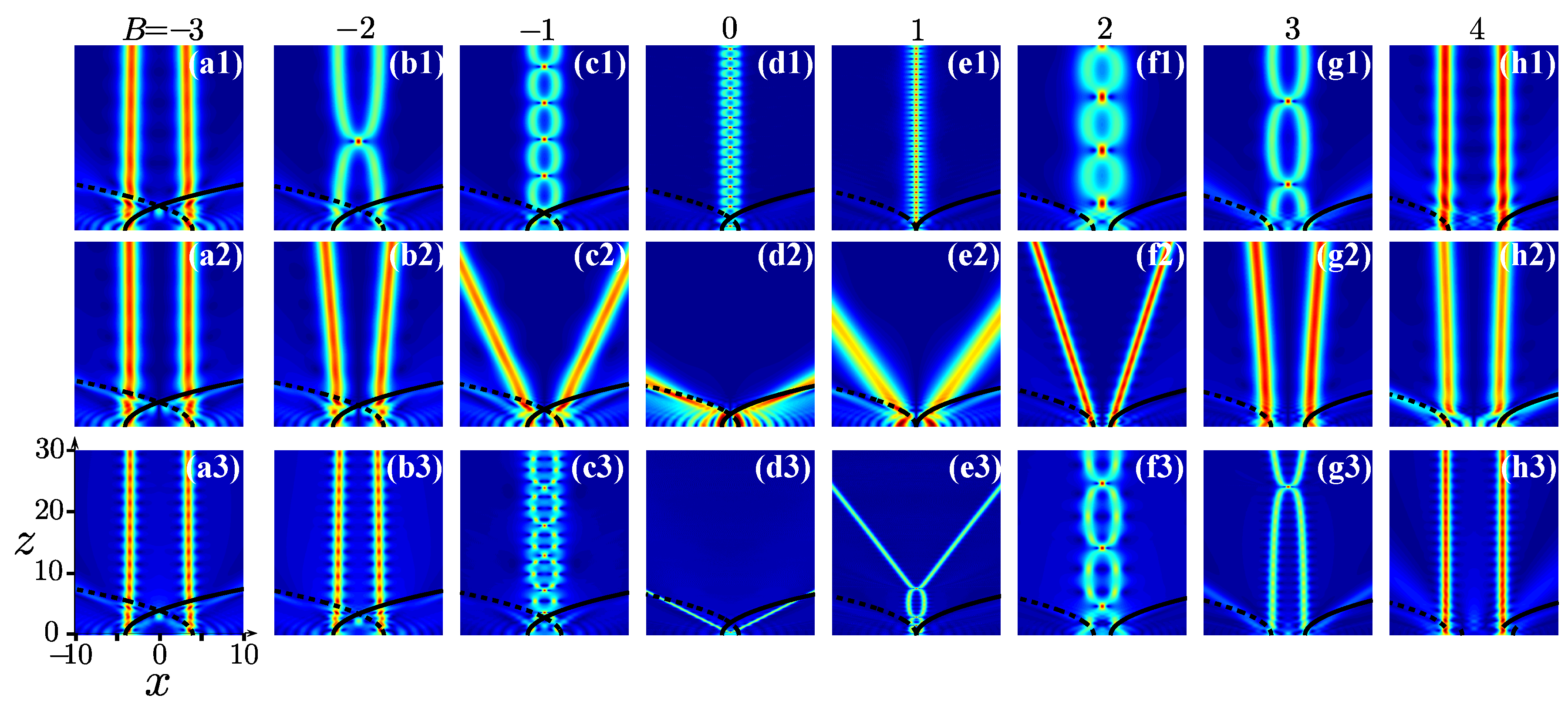
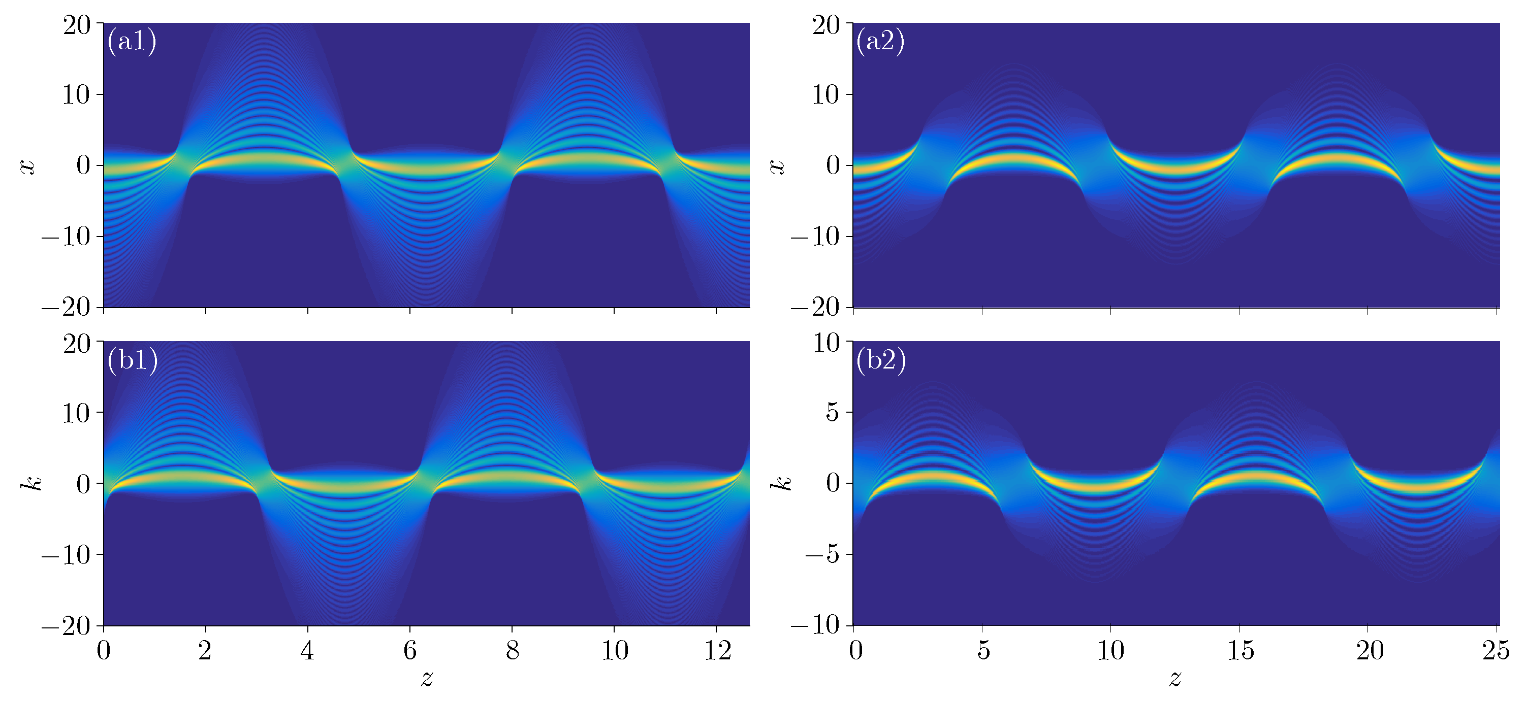
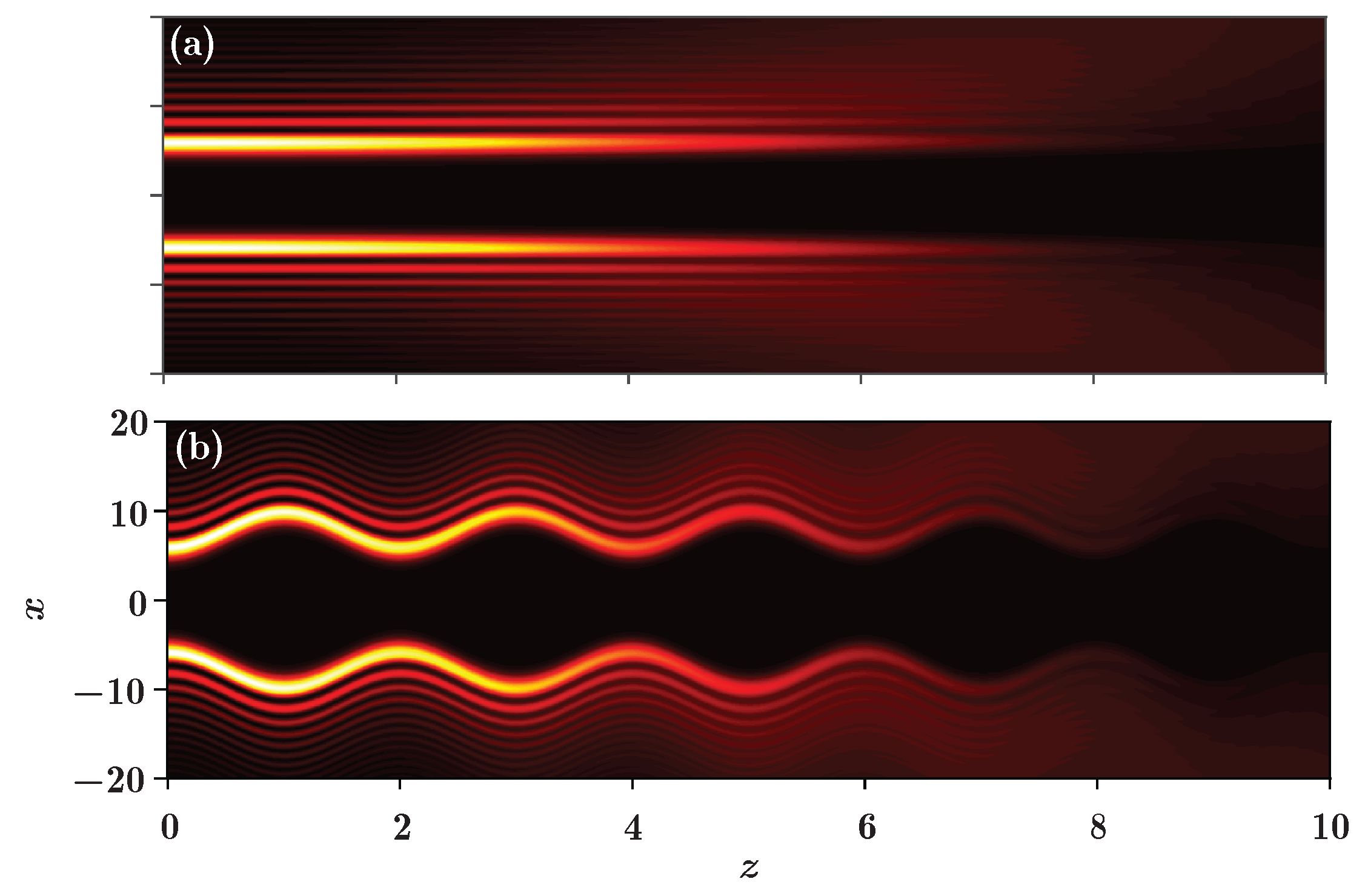
2.2. Harmonic Potential Guidance

In optics and photonics, an external potential embedded in the medium’s index of refraction is often used as an effective tool to modulate light beams. It comes in different forms, as exemplified by vastly different photonic crystal structures. In this subsection, we investigate the management of Airy beams by a harmonic potential added to the linear medium. Typically, such a potential is easily achieved in gradient-index (GRIN) media [61,62] and frequently utilized as a harmonic trap in Bose–Einstein condensates.

2.2.1. One-Dimensional Airy Beams

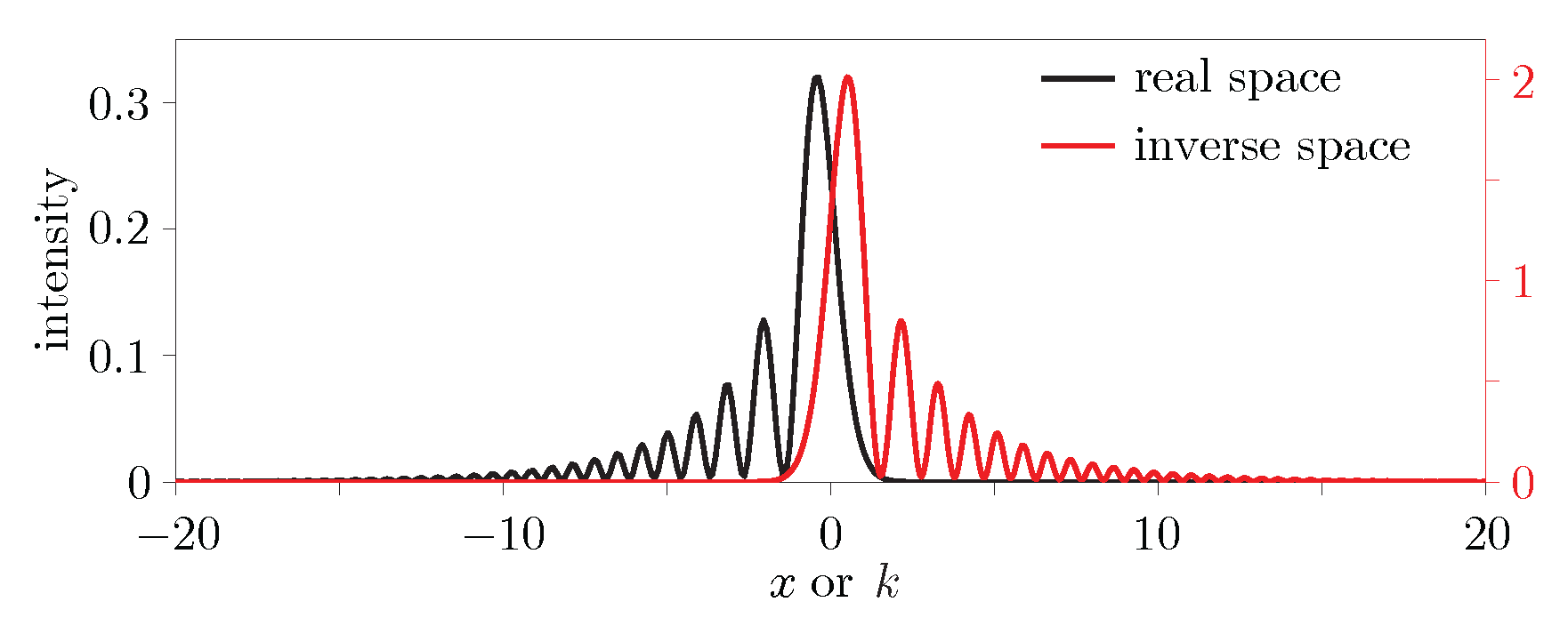
In the one-dimensional (1D) case, the paraxial propagation of a beam in a linear medium with an external harmonic potential is described by the following equation [63,64]:

$$i\frac{\partial \psi }{\partial z}+\frac{1}{2}\frac{{\partial }^2\psi }{\partial x^2}-\frac{1}{2}{\alpha }^2{x}^2\psi =0,$$

(14)

where $\alpha$ determines the width of the harmonic potential. The Fourier transformation (FT) of Equation (14) leads to the corresponding equation in the inverse space:

$$i\frac{\partial \widehat{\psi }}{\partial z}+\frac{1}{2}{\alpha }^2\frac{{\partial }^2\widehat{\psi }}{\partial k^2}-\frac{1}{2}{k}^2\widehat{\psi }=0.$$

(15)

Clearly, if $\alpha =1$, Equations (14) and (15) have the same form, so that both equations have the same solutions but expressed in real (x) and inverse (k) spaces [63], respectively. As before, we are interested in the behavior of Airy beams. The propagation of a truncated Airy beam in the harmonic potential is shown in Figure 3.

Generally, the solution of Equation (14) can be written as [63,64,65,66,67,68,69]:

$$\psi (x,z)={\int }_{-\infty }^{+\infty }\psi (\xi ,0)\sqrt{\mathcal{H}(x,\xi ,z)}d\xi ,$$

(16)

where

$$\begin{array}{c}\hfill \mathcal{H}(x,\xi ,z)=-\frac{i}{2\pi }\alpha csc\left(\alpha z\right)\exp \left\{i\alpha cot\left(\alpha z\right)\left[x^2+{\xi }^2-2x\xi sec\left(\alpha z\right)\right]\right\}\end{array}$$

(17)

is associated with the corresponding kernel. Combining Equations (16) and (17), after some algebra one arrives at

$$\psi (x,z)=f(x,z){\int }_{-\infty }^{+\infty }\left[\psi (\xi ,0)\exp \left(ib{\xi }^2\right)\right]\exp (-iK\xi )d\xi ,$$

(18)

where $b=\frac{\alpha }{2}cot\left(\alpha z\right)$, $K=\alpha xcsc\left(\alpha z\right),$ and

$$\begin{array}{c}\hfill f(x,z)=\sqrt{-\frac{i}{2\pi }\frac{K}{x}}\exp \left(ib{x}^2\right).\end{array}$$

One can see that the integral in Equation (18) is a Fourier transform of $\phi (x,0)\exp (ib{x}^2)$. In other words, the propagation of a beam in a harmonic potential is equivalent to an automatic FT, that is, to the periodic change from the beam to the FT of the beam with a parabolic chirp and back. It is worth mentioning that the same formula also represents a fractional Fourier transform of the initial beam [67,70,71], the “degree” of which is proportional to the propagation distance.

By choosing the input as $\psi (x,0)=Ai(x)\exp (ax)$, the solution in Equation (18) can be found using the following steps:

(i)

Find the Fourier transforms of $\psi (x,0)=\mathrm{Ai}(x)\exp (ax)$ and $\exp (ib{x}^2)$, which can be written as [2,9,63,64]:

$$\widehat{\psi }(k)=\exp \left(-a{k}^2\right)\exp \left[\frac{a^3}{3}+\frac{i}{3}\left(k^3-3a^{2}k\right)\right],$$

(19)

and

$$\sqrt{i\frac{\pi }{b}}\exp \left(-\frac{i}{4b}{k}^2\right),$$

(20)

respectively.

(ii)

Perform the convolution of the two Fourier transforms in Equations (19) and (20), and using the definition [72]

$$\mathrm{Ai}(x)=\frac{1}{2\pi i}{\int }_{-i\infty }^{+i\infty }\exp \left(xt-\frac{t^3}{3}\right)dt,$$

find the inverse Fourier transform:

$$\begin{array}{cc}\hfill \psi (x,z)=& -f(x,z)\sqrt{i\frac{\pi }{b}}\exp \left(\frac{a^3}{3}\right)\mathrm{Ai}\left(\frac{K}{2b}-\frac{1}{16b^2}+i\frac{a}{2b}\right)\hfill \\ & \times \exp \left[\left(a+\frac{i}{4b}\right)\left(\frac{K}{2b}-\frac{1}{16b^2}+i\frac{a}{2b}\right)\right]\exp \left[-i\frac{K^2}{4b}-\frac{1}{3}{\left(a+\frac{i}{4b}\right)}^3\right].\hfill \end{array}$$

(21)

From this expression, one obtains the accelerating trajectory of the initial beam:

$$x=\frac{1}{4{\alpha }^2}\frac{{\sin }^2(\alpha z)}{\cos (\alpha z)},$$

(22)

with the period $D=2\pi /\alpha$. Here, $z\ne (2m+1)\mathcal{D}/4$, where m is a positive integer. This trajectory is ideal, because it indicates that the Airy beam can accelerate all the way to infinity $x\to \pm \infty$, when $z\to (2m+1)D/4$. However, upon exponential apodization of the Airy beam, such an acceleration will stop when z is close to the points mentioned. At these points, the beam will turn around, accelerate in the opposite direction, and change the shape. We call these points the phase transition points, for the reasons explained below.

So, several issues concerning Equation (21) must be addressed:

(i)

When $z=m\mathcal{D}$, we have $\psi (x,z)=\psi (x,0)$—an initial beam recurrence.

(ii)

When $z=(2m+1)\mathcal{D}/2$, we have $\psi (x,z)=\psi (-x,0)$—an inversion of the initial beam.

(iii)

When $z=(2m+1)\mathcal{D}/4$, by directly solving Equation (18) for the FT of the initial beam, we have

$$\psi \left(x,z=\frac{2m+1}{4}\mathcal{D}\right)=\sqrt{-i\frac{s\alpha }{2\pi }}\exp \left(-a{\alpha }^2{x}^2\right)\exp \left[\frac{a^3}{3}+i\frac{s}{3}\left({\alpha }^3{x}^3-3a^2\alpha x\right)\right],$$

(23)

where $s=1$ if m is even and $s=-1$ if m is odd. This field is unrelated to the initial Airy beam—that is, it represents a new “phase” of the propagating beam.

Equation (23) displays a Gaussian intensity profile, which is completely different from the intensity profiles elsewhere during propagation. It is similar to the propagating Gaussian pulse as it bounces off the harmonic potential wall—but the Gaussian beam remains Gaussian in propagation, whereas this pulse inverts and becomes an inverse Airy beam. On the other hand, it is different from a free Gaussian wave packet hitting an infinite potential wall—there, during the bounce, the packet becomes a rapidly oscillating multi-peaked structure, owing to the interference between the incoming and the reflected beam. Since the inversion introduces a discontinuity in the velocity and a singularity in the acceleration, for lack of a better word, we refer to the phenomenon as the phase transition of the finite energy Airy beam, due to the harmonic potential. Correspondingly, $z=(2m+1)\mathcal{D}/4$ are the phase transition points.

When we introduce a transverse displacement $x_0$ of the beam, the initial beam is $\psi (x,0)=Ai(x-x_0)\exp [a(x-x_0)]$, and the solution can be written as:

$$\begin{array}{}& \hfill \psi (x,z)=& -f(x,z)\sqrt{i\frac{\pi }{b}}\exp \left(\frac{a^3}{3}\right)\mathrm{Ai}\left(\frac{K}{2b}-\frac{1}{16b^2}+i\frac{a}{2b}-x_0\right)\hfill (24)& & \times \exp \left[\left(a+\frac{i}{4b}\right)\left(\frac{K}{2b}-\frac{1}{16b^2}+i\frac{a}{2b}-x_0\right)\right]\exp \left[-i\frac{K^2}{4b}-\frac{1}{3}{\left(a+\frac{i}{4b}\right)}^3\right].\hfill \end{array}$$

The corresponding trajectory is:

$$x=\frac{1}{4{\alpha }^2}\frac{{\sin }^2(\alpha z)}{\cos (\alpha z)}+x_0\cos (\alpha z),$$

(25)

At the transition points, we have:

$$\begin{array}{c}\hfill \psi \left(x,z=\frac{2m+1}{4}\mathcal{D}\right)=\sqrt{-i\frac{s\alpha }{2\pi }}\exp (-i{x}_0\alpha x)\exp \left(-a{\alpha }^2{x}^2\right)\exp \left[\frac{a^3}{3}+i\frac{s}{3}\left({\alpha }^3{x}^3-3a^2\alpha x\right)\right].\end{array}$$

(26)

Comparing with the former case, the transverse displacement introduces a linear chirp at the transition points. There is no change of the period and phase transition points, so one can predict that the beam executes the same motion as before, but it is transversely stretched. One can also predict that with an increasing transverse displacement $|x_0|$, the beam will accelerate along an ever more elongated cosine curve.

To explore the phase transition region more clearly, we show the numerical simulations of trajectories, velocities, and accelerations of the beam during propagation in Figure 4, for different cases. One can observe that the accelerating trajectories are modulated by the transverse displacement; the beam acceleration with $x_0<0$ being opposite to the case with $x_0>0$. In addition, the beam inversion produces a discontinuity in the velocity and a singularity in the acceleration, which demonstrates nicely that the motion is not harmonic and that there exist two phase regions: the Airy phase and the single-peak phase. According to Equations (24) and (26), the single-peak structure only occurs at the phase transition points; before and after these points, the beam still exhibits multi-peak structure, having to reconnect the accelerating motion before the point with the decelerating motion after the point. The length of the single-peak phase is determined by the size of the decay parameter, as displayed in Figure 4b; the smaller a, the smaller the length, and the harder it is for the beam to make a sudden inversion, so the region in Figure 4c is narrower than that in Figure 4d. However, $x_0$ has no effect on the width of the single-peak phase region when a is fixed.

We next consider the initial beam with a linear chirp:

$$\psi (x,0)=\mathrm{Ai}(x-x_0)\exp [a(x-x_0)]\exp (i\beta x),$$

(27)

with $\beta$ being the constant wavenumber. Thus, the solution is written as:

$$\begin{array}{cc}\hfill \psi (x,z)=& -f(x,z)\sqrt{i\frac{\pi }{b}}\exp \left(\frac{a^3}{3}\right)\mathrm{Ai}\left(\frac{K^{\prime }}{2b}-\frac{1}{16b^2}+i\frac{a}{2b}-x_0\right)\hfill \\ & \times \exp \left[\left(a+\frac{i}{4b}\right)\left(\frac{K^{\prime }}{2b}-\frac{1}{16b^2}+i\frac{a}{2b}-x_0\right)\right]\exp \left[-i\frac{K^{\prime 2}}{4b}-\frac{1}{3}{\left(a+\frac{i}{4b}\right)}^3\right],\hfill \end{array}$$

(28)

with $K^{\prime }=K-\beta$. Clearly, the period $\mathcal{D}$ does not change and the phase transition point is still an odd integer multiple of the quarters of the period. Mathematically, the trajectory is given by

$$x=\frac{1}{4{\alpha }^2}\frac{{\sin }^2(\alpha z)}{\cos (\alpha z)}+x_0\cos (\alpha z)+\frac{\beta }{\alpha }\sin (\alpha z),$$

and is modulated greatly by the linear chirp. At the phase transition points, we have:

$$\begin{array}{cc}\hfill \psi \left(x,z=\frac{2m+1}{4}\mathcal{D}\right)=& \sqrt{-i\frac{s\alpha }{2\pi }}\exp [-i{x}_0(\alpha x-\beta )]\exp \left[-a{(\alpha x-\beta )}^2\right]\hfill \\ & \times \exp \left\{\frac{a^3}{3}+i\frac{s}{3}\left[{(\alpha x-\beta )}^3-3a^2(\alpha x-\beta )\right]\right\}.\hfill \end{array}$$

(29)

In this case, the beam is equivalent to an obliquely incident beam, but without the ballistic properties due to the harmonic potential [3,73].

If the initial finite energy Airy beam carries a quadratic chirp,

$$\psi (x,0)=\mathrm{Ai}(x-x_0)\exp \left[a(x-x_0)\right]\exp \left(i\beta x^2\right),$$

(30)

the analytical solution will be

$$\begin{array}{cc}\hfill \psi (x,z)=& -f(x,z)\sqrt{i\frac{\pi }{b^{\prime }}}\exp \left(\frac{a^3}{3}\right)\mathrm{Ai}\left(\frac{K}{2b^{\prime }}-\frac{1}{16b^{\prime 2}}+i\frac{a}{2b^{\prime }}-x_0\right)\hfill \\ & \times \exp \left[\left(a+\frac{i}{4b^{\prime }}\right)\left(\frac{K}{2b^{\prime }}-\frac{1}{16b^{\prime 2}}+i\frac{a}{2b^{\prime }}-x_0\right)\right]\exp \left[-i\frac{K^2}{4b^{\prime }}-\frac{1}{3}{\left(a+\frac{i}{4b^{\prime }}\right)}^3\right].\hfill \end{array}$$

(31)

Here, $b^{\prime }=b+\beta$, but the period in this case is still $\mathcal{D}$. However, the phase transition points are not the same as before; they are obtained as:

$$z=\frac{1}{\alpha }arctan\left(-\frac{\alpha }{2\beta }\right)+\frac{m}{2}\mathcal{D}.$$

(32)

Concerning the trajectory, it is now:

$$x=\frac{{\sin }^2(\alpha z)}{4\alpha [\alpha \cos (\alpha z)+2\beta \sin (\alpha z)]}+[\alpha \cos (\alpha z)+2\beta \sin (\alpha z)]x_0,$$

(33)

and obviously, the influence from the quadratic chirp is not negligible.

Comparing these two chirped cases, we note that in both cases the trajectories are modulated greatly. In the linear chirp case, the phase transition points and the period do not change, but the beam at the phase transition point has a transverse displacement. While in the quadratic chirp case, the phase transition point is moved, but the beam profile is not affected.

By now, it is apparent that the propagation of beams according to the linear Schrödinger equation with parabolic potential is intimately connected with the self-Fourier (SF) transform. Generally, for an arbitrary $\psi (x)$ propagating to $\pi /4$ in a harmonic potential, an SF beam will be obtained at that point [74]. Here, when a truncated Airy beam $\phi (x)=Ai(x)\exp (ax)$ propagates to $z=\pi /(4\alpha )$, we find the corresponding Fourier transform pair:

$$\mathcal{F}[\psi (x)](k)=\sqrt{\frac{2\pi }{\alpha }}\psi \left(-\frac{k}{\alpha }\right).$$

(34)

Therefore, the expression for the self-Fourier beam is:

$$\begin{array}{}& \hfill \psi (x)=-\sqrt[4]{2}\mathrm{Ai}\left(\sqrt{2}x-\frac{1}{4{\alpha }^2}+i\frac{a}{\alpha }\right)& \exp \left[a\left(\sqrt{2}x-\frac{1}{2{\alpha }^2}\right)\right]\times \hfill (35)& & \exp \left[-\frac{i}{2}\left(2\alpha x^2-\frac{\sqrt{2}}{\alpha }x+\frac{a^2}{\alpha }+\frac{1}{6{\alpha }^3}\right)\right].\hfill \end{array}$$

In Figure 5, the intensity of the SF beam is shown by the black curve, and the corresponding intensity in Fourier space is shown by the red curve. One can see that the beam profiles are the same except for the inversion, which is in accordance with the theoretical result presented in Equation (34). This way of generating SF beams is universal, it does not depend on the form of the initial beam. Furthermore, we have recently demonstrated that the linear and nonlinear Talbot effects might be interpreted as a fractional SF or a regular SF transform phenomenon, respectively [75,76]. Such SF beams may find potential applications in optical information processing, routing, and switching.

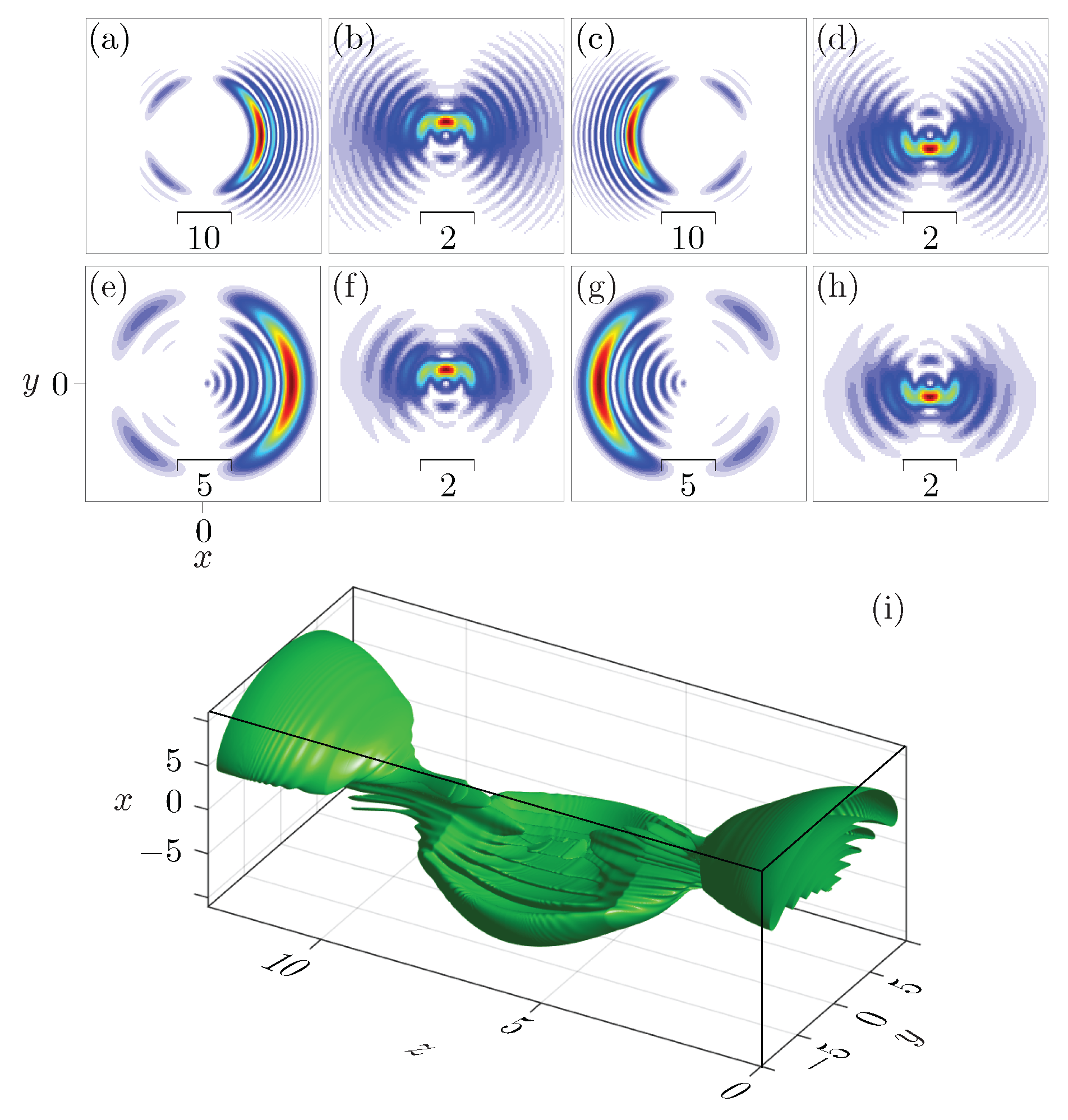
2.2.2. Two-Dimensional Case

Naturally, the harmonic oscillator model in Equation (14) is easily extended to two, three or even four dimensions [64]. In 2D, it has the form:

$$i\frac{\partial \psi }{\partial z}+\frac{1}{2}\left(\frac{{\partial }^2\psi }{\partial x^2}+\frac{{\partial }^2\psi }{\partial y^2}\right)-\frac{1}{2}{\alpha }^2\left(x^2+y^2\right)\psi =0,$$

(36)

with the initial beam being:

$$\psi (x,y,z=0)=\mathrm{Ai}(x)\mathrm{Ai}(y)\exp [a(x+y)].$$

(37)

By the separation of variables, the 2D problem can be reduced to two 1D cases [64,77]. The result is displayed in Figure 6. Similar to the 1D case, the 2D Airy beam displays inversion and phase transition (the gaps represent the single-peak regions) during propagation. From Figure 6c,d, one can clearly see that the beam at $z=\pi /(4\alpha )$ is still an SF beam, just like in the 1D case. Thus, the wave function is a product of two finite-energy Airy beams: one along x and the other along the y direction. In a 2D parabolic potential, the wave exhibits all the properties of 1D Airy beams: periodic inversion, phase transition, and anharmonic oscillation.

For the cases that cannot be treated with the variable separation method, e.g., when the initial beam is a superposition of AAF beams carrying orbital angular momentum [18,41,42,45,78], in the radially symmetric case one can switch to the polar coordinates. Then, the input can be written as:

$$\psi (r,\theta )=\mathrm{Ai}[\pm (r_0-r)]\exp [\pm a(r_0-r)]{\displaystyle \sum _{n=1}^4}\exp (in\theta ),$$

(38)

where ± represents the inward and outward AAF beams, $r_0$ determines the location of the main ring, and $\theta$ represents the spatial frequency in polar coordinates. An analytical propagating solution of Equation (38) is hard to obtain. However, using a fairly accurate approximation method developed in [18,79], the AAF beam propagation can be described as a superposition of Bessel beams:

$$\begin{array}{c}\hfill \psi (r,\theta ,z)\approx -A_{0}f(r,\theta ,z)\exp \left(ib{r}_0^2\right){\displaystyle \sum _{n=1}^4}{i}^{1-n}\exp (in\theta )J_n(r_{0}r),\end{array}$$

(39)

where $A_0\approx (1-a^2/r_0)\exp (a^3/3)$. The results are depicted in Figure 7. The first row of panels presents the intensity of an outward AAF beam; the second row of panels presents the intensity of an inward AAF beam.

In the 3D plot, one can see that the oscillation is more continuous, and there are no phase transition points.

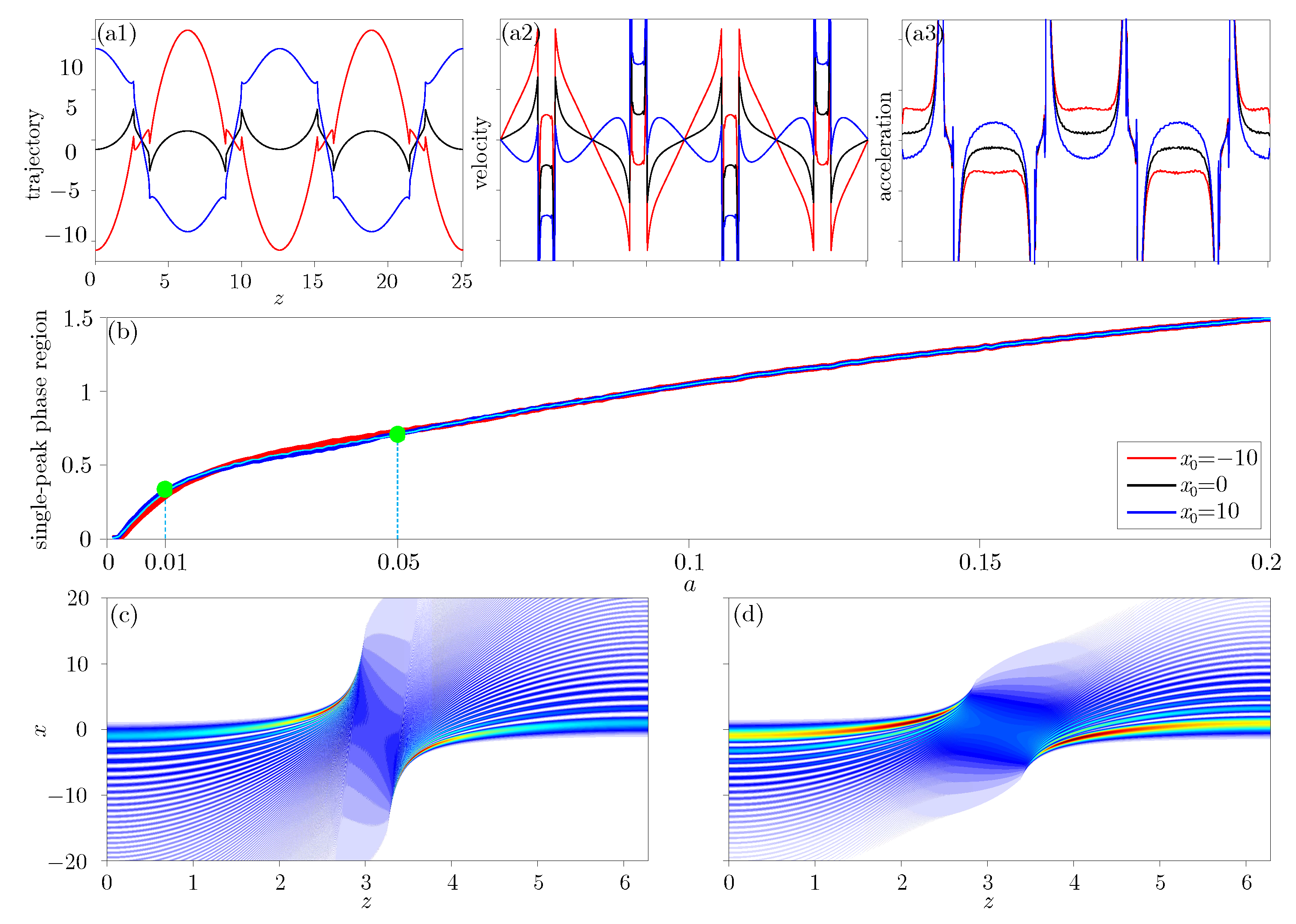
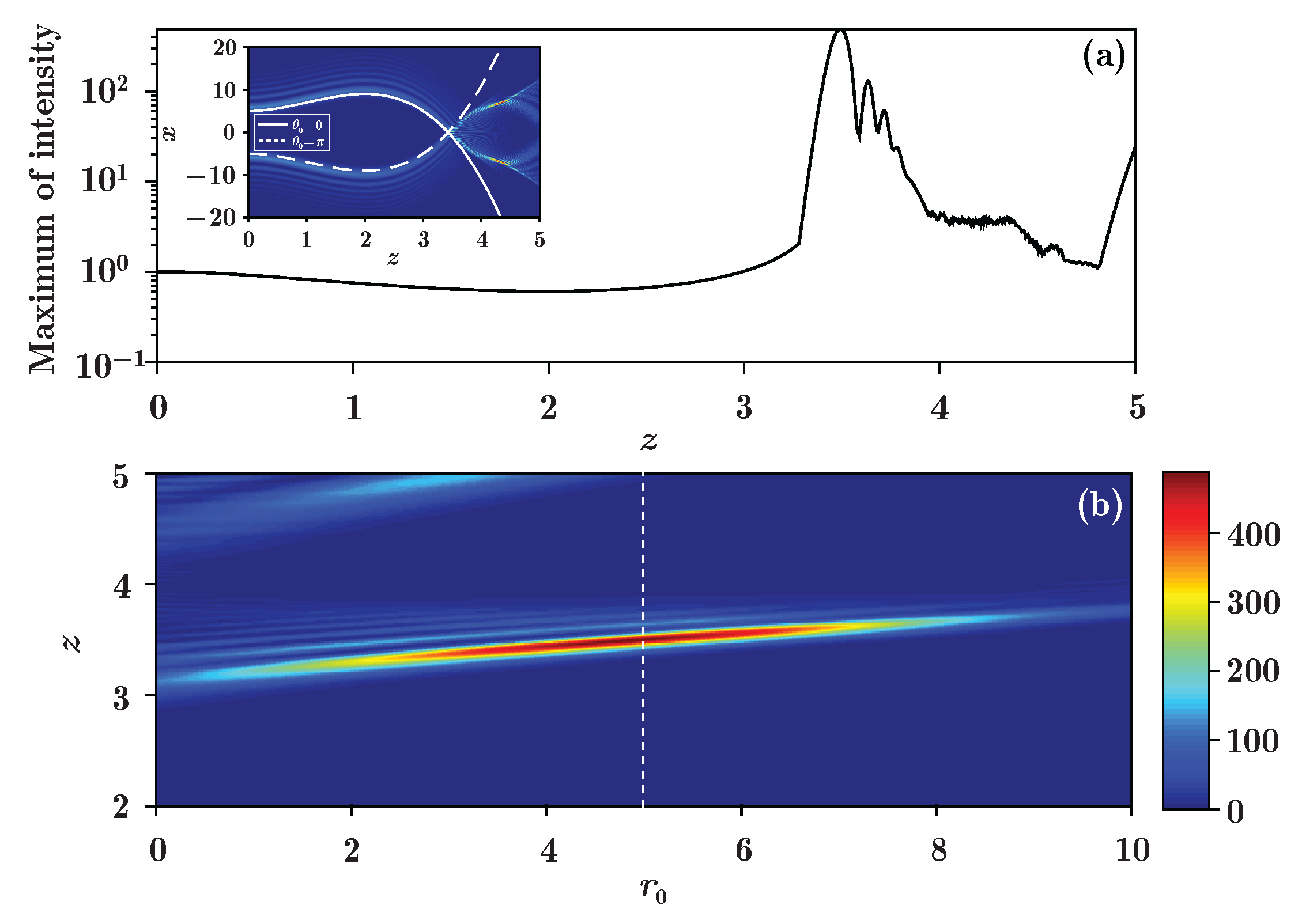
2.3. Dynamic Linear Potential Guidance

As mentioned in the introduction, the AAF beams are radially symmetric beams that possess autofocusing property. It has been shown that the propagation trajectory as well as the positions of autofocusing points of the AAF beams can be controlled by potentials [41]. In our investigation [80], we theoretically analyzed the propagation and autofocusing effect of the AAF beams in a dynamic linear potential. We found that the linear potential may weaken (even eliminate) or strengthen the autofocusing effect of the AAF beams, depending on the form of the linear potential. In this case, the governing equation is written as [41,81,82]:

$$i\frac{d\psi }{dz}+\frac{1}{2}\left(\frac{{\partial }^2\psi }{\partial r^2}+\frac{1}{r}\frac{\partial \psi }{\partial r}\right)-\frac{d(z)}{2}r\psi =0.$$

(40)

Here, the external potential is linear in r, with the scaling factor d that depends on the longitudinal coordinate; this is the so-called dynamical linear potential [81,82]. Again, it is hard to find an analytical solution of Equation (40), so we resort to an approximate analysis, by introducing an azimuthal modulation of the inward AAF beam:

$${\psi }_{\mathrm{az}}(x,y)=\mathrm{Ai}(r_0-r)\exp [a(r_0-r)]\exp \left(-\frac{{(\theta -{\theta }_0)}^2}{w_0^2}\right),$$

(41)

with $w_0$ being the width of the modulation, $\theta =arctan(y/x)$ being the azimuthal angle, ${\theta }_0$ representing the modulation direction. If the value of $w_0$ is small enough, the azimuthal modulation will result in a very narrow structure, so with $w_0\to 0$ the result will be quite similar to the one-dimensional finite-energy Airy beam. In this way, the AAF beam can be transferred into the 1D finite-energy Airy beam [81,83], as:

$$\psi (x,y)={\displaystyle \sum _{{\theta }_0=-\pi }^{+\pi }}\mathrm{Ai}(r_0-x_p)\exp [a(r_0-x_p)].$$

(42)

Thus, by an analogy with the analytical result in [81], we describe the autofocusing effect and the propagation of the AAF beam as follows:

$$\begin{array}{cc}\hfill \psi (x,y,z)=C& {\displaystyle \sum _{{\theta }_0=-\pi }^{+\pi }}\mathrm{Ai}\left[iaz+\left(\frac{1}{2}{f}_1-\frac{1}{4}{z}^2+(r_0-x_p)\right)\right]\exp \left[a\left(\frac{1}{2}{f}_1-\frac{1}{2}{z}^2+(r_0-x_p)\right)\right]\times \hfill \\ & \exp \left[i\left(\frac{1}{2}{a}^{2}z+\frac{1}{4}z{f}_1-\frac{1}{8}{f}_2-\frac{1}{12}{z}^3-\frac{1}{2}(r_0-x_p)g+\frac{1}{2}(r_0-x_p)z\right)\right],\hfill \end{array}$$

(43)

where, $g(z)={\int }_0^{z}d(t)dt$, $f_1(z)=f_0+{\int }_0^{z}g(t)dt$ and $f_2(z)={\int }_0^z{g}^2(t)dt$. The trajectory of each component in a linear dynamic potential is

$$x_p=r_0+\frac{1}{2}{f}_1-\frac{1}{4}{z}^2.$$

(44)

Clearly, the AAF beam can be effectively manipulated by the linear potential.

If there is no autofocusing during propagation, Equation (43) can be reduced to the following form:

$$\begin{array}{cc}\hfill \psi (x,y,z)=& \mathrm{Ai}\left[iaz+\left(\frac{1}{2}{f}_1-\frac{1}{4}{z}^2+(r_0-r)\right)\right]\exp \left[a\left(\frac{1}{2}{f}_1-\frac{1}{2}{z}^2+(r_0-r)\right)\right]\times \hfill \\ & \exp \left[i\left(\frac{1}{2}{a}^{2}z+\frac{1}{4}z{f}_1-\frac{1}{8}{f}_2-\frac{1}{12}{z}^3-\frac{1}{2}(r_0-r)g+\frac{1}{2}(r_0-r)z\right)\right],\hfill \end{array}$$

(45)

which becomes invalid when autofocusing happens. In this way, using Equations (43) and (45), the propagation of an AAF beam manipulated by a dynamic linear potential can now be reduced to a simple 1D case.

When we set $d(z)=1$, the trajectory of the beam is $x_p=r_0$, that is, a straight line, so the autofocusing does not occur during propagation, and the propagation can be described by Equation (45). For this case, the linear potential exerts a “pulling” influence that can balance the virtual force which makes the beam focus. While, if the potential is a periodic function $d(z)=1+4{\pi }^2\cos (\pi z)$, as in the former case, the potential also exerts a pulling effect, and the trajectory is a cosine-like curve, which is also periodic. The corresponding results are displayed in Figure 8.

For the case with $d(z)=13-12z$, from the corresponding trajectory $x_p=r_0-z^3+3z^2$, we know that the beam will undergo autofocusing during propagation, so the process should be described by Equation (43). From the inset in Figure 9, the two components (${\theta }_0=0$, ${\theta }_0=\pi$) separate before the focusing point, and then converge. Since the slope of the components at the colliding point is much bigger than without a potential, as in [40], this can be viewed as the components acquiring a larger speed because of the “pushing” effect, hence the autofocusing is strengthened. Similar to the former study, the maximum of the beam intensity (MBI) is also a function of both $r_0$ and the propagation distance, as displayed in Figure 9b; the MBI first increases and then decreases with the increasing of $r_0$. Besides this effect, one can also see that the location of the MBI also changes with $r_0$, the reason being that the autofocusing effect requires a longer distance to establish itself when $r_0$ increases. As stated above, the transverse and longitudinal coordinates are normalized to some characteristic transverse width $x_0$ and the corresponding Rayleigh range $k{x}_0^2$. The unit of intensity of the beam is arbitrary.

3. Conclusions

In conclusion, in this short review, we have briefly discussed the origin and the fundamental developments concerning Airy beams, and made a systematic review of the modulation of Airy beams under the guidance of nonlinearity and different potentials. This review is based on our recently published work. Our investigations will hopefully attract researchers who work on the related phenomena in other fields. Thus, the results presented here are not just limited to optics, but can lead to potential applications in biology, particle manipulation, microparticle trapping, Bose–Einstein condensates, signal processing and manipulating, and other disciplines. Actually, the Airy and other self-accelerating beams are among the hottest topics in optics. The investigations related to such beams are interesting and show impressive progress. Still, there are many unknown and important phenomena to be researched and new effects to be discovered concerning the accelerating beams.

References

1. Berry, M.V.; Balazs, N.L. Nonspreading wave packets. Am. J. Phys. 1979, 47, 264–267. [Google Scholar] [CrossRef]
2. Siviloglou, G.A.; Christodoulides, D.N. Accelerating finite energy Airy beams. Opt. Lett. 2007, 32, 979–981. [Google Scholar] [CrossRef] [PubMed]
3. Siviloglou, G.A.; Broky, J.; Dogariu, A.; Christodoulides, D.N. Ballistic dynamics of Airy beams. Opt. Lett. 2008, 33, 207–209. [Google Scholar] [CrossRef] [PubMed]
4. Minovich, A.; Klein, A.E.; Janunts, N.; Pertsch, T.; Neshev, D.N.; Kivshar, Y.S. Generation and Near-Field Imaging of Airy Surface Plasmons. Phys. Rev. Lett. 2011, 107, 116802. [Google Scholar] [CrossRef] [PubMed]
5. Li, L.; Li, T.; Wang, S.M.; Zhang, C.; Zhu, S.N. Plasmonic Airy Beam Generated by In-Plane Diffraction. Phys. Rev. Lett. 2011, 107, 126804. [Google Scholar] [CrossRef] [PubMed]
6. Lin, Z.; Guo, X.; Tu, J.; Ma, Q.; Wu, J.; Zhang, D. Acoustic non-diffracting Airy beam. J. Appl. Phys. 2015, 117, 104503. [Google Scholar] [CrossRef]
7. Fu, S.; Tsur, Y.; Zhou, J.; Shemer, L.; Arie, A. Propagation Dynamics of Airy Water-Wave Pulses. Phys. Rev. Lett. 2015, 115, 034501. [Google Scholar] [CrossRef] [PubMed]
8. Bar-Ziv, U.; Postan, A.; Segev, M. Observation of shape-preserving accelerating underwater acoustic beams. Phys. Rev. B 2015, 92, 100301. [Google Scholar] [CrossRef]
9. Siviloglou, G.; Broky, J.; Dogariu, A.; Christodoulides, D. Observation of Accelerating Airy Beams. Phys. Rev. Lett. 2007, 99, 213901. [Google Scholar] [CrossRef] [PubMed]
10. Polynkin, P.; Kolesik, M.; Moloney, J.V.; Siviloglou, G.A.; Christodoulides, D.N. Curved plasma channel generation using ultraintense Airy beams. Science 2009, 324, 229–232. [Google Scholar] [CrossRef] [PubMed]
11. Salandrino, A.; Christodoulides, D.N. Airy plasmon: A nondiffracting surface wave. Opt. Lett. 2010, 35, 2082–2084. [Google Scholar] [CrossRef] [PubMed]
12. Liang, Y.; Hu, Y.; Song, D.; Lou, C.; Zhang, X.; Chen, Z.; Xu, J. Image signal transmission with Airy beams. Opt. Lett. 2015, 40, 5686–5689. [Google Scholar] [CrossRef] [PubMed]
13. Jia, S.; Vaughan, J.C.; Zhuang, X. Isotropic three-dimensional super-resolution imaging with a self-bending point spread function. Nat. Photon. 2014, 8, 302–306. [Google Scholar] [CrossRef] [PubMed]
14. Polynkin, P.; Kolesik, M.; Moloney, J. Filamentation of Femtosecond Laser Airy Beams in Water. Phys. Rev. Lett. 2009, 103, 123902. [Google Scholar] [CrossRef] [PubMed]
15. Zheng, Z.; Zhang, B.F.; Chen, H.; Ding, J.; Wang, H.T. Optical trapping with focused Airy beams. Appl. Opt. 2011, 50, 43–49. [Google Scholar] [CrossRef] [PubMed]
16. Cao, R.; Yang, Y.; Wang, J.; Bu, J.; Wang, M.; Yuan, X.C. Microfabricated continuous cubic phase plate induced Airy beams for optical manipulation with high power efficiency. Appl. Phys. Lett. 2011, 99, 261106. [Google Scholar] [CrossRef]
17. Baumgartl, J.; Mazilu, M.; Dholakia, K. Optically mediated particle clearing using Airy wavepackets. Nat. Photon. 2008, 2, 675–678. [Google Scholar] [CrossRef]
18. Zhang, P.; Prakash, J.; Zhang, Z.; Mills, M.S.; Efremidis, N.K.; Christodoulides, D.N.; Chen, Z. Trapping and guiding microparticles with morphing autofocusing Airy beams. Opt. Lett. 2011, 36, 2883–2885. [Google Scholar] [CrossRef] [PubMed]
19. Schley, R.; Kaminer, I.; Greenfield, E.; Bekenstein, R.; Lumer, Y.; Segev, M. Loss-proof self-accelerating beams and their use in non-paraxial manipulation of particles’ trajectories. Nat. Commun. 2014, 5, 5189. [Google Scholar] [CrossRef] [PubMed]
20. Vettenburg, T.; Dalgarno, H.I.; Nylk, J.; Coll-Lladó, C.; Ferrier, D.E.; Čižmár, T.; Gunn-Moore, F.J.; Dholakia, K. Light-sheet microscopy using an Airy beam. Nat. Meth. 2014, 11, 541–544. [Google Scholar] [CrossRef] [PubMed]
21. Abdollahpour, D.; Suntsov, S.; Papazoglou, D.G.; Tzortzakis, S. Spatiotemporal Airy Light Bullets in the Linear and Nonlinear Regimes. Phys. Rev. Lett. 2010, 105, 253901. [Google Scholar] [CrossRef] [PubMed]
22. Chong, A.; Renninger, W.H.; Christodoulides, D.N.; Wise, F.W. Airy-Bessel wave packets as versatile linear light bullets. Nat. Photon. 2010, 4, 103–106. [Google Scholar] [CrossRef]
23. Ament, C.; Polynkin, P.; Moloney, J.V. Supercontinuum Generation with Femtosecond Self-Healing Airy Pulses. Phys. Rev. Lett. 2011, 107, 243901. [Google Scholar] [CrossRef] [PubMed]
24. Kim, K.Y.; Hwang, C.Y.; Lee, B. Slow non-dispersing wavepackets. Opt. Express 2011, 19, 2286–2293. [Google Scholar] [CrossRef] [PubMed]
25. Voloch-Bloch, N.; Lereah, Y.; Lilach, Y.; Gover, A.; Arie, A. Generation of electron Airy beams. Nature 2013, 494, 331–335. [Google Scholar] [CrossRef] [PubMed]
26. Gu, Y.; Gbur, G. Scintillation of Airy beam arrays in atmospheric turbulence. Opt. Lett. 2010, 35, 3456–3458. [Google Scholar] [CrossRef] [PubMed]
27. Baumgartl, J.; Čižmár, T.; Mazilu, M.; Chan, V.C.; Carruthers, A.E.; Capron, B.A.; McNeely, W.; Wright, E.M.; Dholakia, K. Optical path clearing and enhanced transmission through colloidal suspensions. Opt. Express 2010, 18, 17130–17140. [Google Scholar] [CrossRef] [PubMed]
28. Zhao, J.; Chremmos, I.D.; Song, D.; Christodoulides, D.N.; Efremidis, N.K.; Chen, Z. Curved singular beams for three-dimensional particle manipulation. Sci. Rep. 2015, 5, 12086. [Google Scholar] [CrossRef] [PubMed]
29. Libster-Hershko, A.; Epstein, I.; Arie, A. Rapidly Accelerating Mathieu and Weber Surface Plasmon Beams. Phys. Rev. Lett. 2014, 113, 123902. [Google Scholar] [CrossRef] [PubMed]
30. Ellenbogen, T.; Voloch-Bloch, N.; Ganany-Padowicz, A.; Arie, A. Nonlinear generation and manipulation of Airy beams. Nat. Photon. 2009, 3, 395–398. [Google Scholar] [CrossRef]
31. Lotti, A.; Faccio, D.; Couairon, A.; Papazoglou, D.G.; Panagiotopoulos, P.; Abdollahpour, D.; Tzortzakis, S. Stationary nonlinear Airy beams. Phys. Rev. A 2011, 84, 021807. [Google Scholar] [CrossRef]
32. Fattal, Y.; Rudnick, A.; Marom, D.M. Soliton shedding from Airy pulses in Kerr media. Opt. Express 2011, 19, 17298–17307. [Google Scholar] [CrossRef] [PubMed]
33. Rudnick, A.; Marom, D.M. Airy-soliton interactions in Kerr media. Opt. Express 2011, 19, 25570–25582. [Google Scholar] [CrossRef] [PubMed]
34. Zhang, Y.Q.; Belić, M.; Wu, Z.K.; Zheng, H.B.; Lu, K.Q.; Li, Y.Y.; Zhang, Y.P. Soliton pair generation in the interactions of Airy and nonlinear accelerating beams. Opt. Lett. 2013, 38, 4585–4588. [Google Scholar] [CrossRef] [PubMed]
35. Zhang, Y.Q.; Belić, M.R.; Zheng, H.B.; Chen, H.X.; Li, C.B.; Li, Y.Y.; Zhang, Y.P. Interactions of Airy beams, nonlinear accelerating beams, and induced solitons in Kerr and saturable nonlinear media. Opt. Express 2014, 22, 7160–7171. [Google Scholar] [CrossRef] [PubMed]
36. Kaminer, I.; Segev, M.; Christodoulides, D.N. Self-Accelerating Self-Trapped Optical Beams. Phys. Rev. Lett. 2011, 106, 213903. [Google Scholar] [CrossRef] [PubMed]
37. Panagiotopoulos, P.; Abdollahpour, D.; Lotti, A.; Couairon, A.; Faccio, D.; Papazoglou, D.G.; Tzortzakis, S. Nonlinear propagation dynamics of finite-energy Airy beams. Phys. Rev. A 2012, 86, 013842. [Google Scholar] [CrossRef]
38. Hu, Y.; Huang, S.; Zhang, P.; Lou, C.; Xu, J.; Chen, Z. Persistence and breakdown of Airy beams driven by an initial nonlinearity. Opt. Lett. 2010, 35, 3952–3954. [Google Scholar] [CrossRef] [PubMed]
39. Chen, R.P.; Yin, C.F.; Chu, X.X.; Wang, H. Effect of Kerr nonlinearity on an Airy beam. Phys. Rev. A 2010, 82, 043832. [Google Scholar] [CrossRef]
40. Efremidis, N.K.; Christodoulides, D.N. Abruptly autofocusing waves. Opt. Lett. 2010, 35, 4045–4047. [Google Scholar] [CrossRef] [PubMed]
41. Hwang, C.Y.; Kim, K.Y.; Lee, B. Dynamic Control of Circular Airy Beams With Linear Optical Potentials. IEEE Photon. J. 2012, 4, 174–180. [Google Scholar] [CrossRef]
42. Hwang, C.Y.; Kim, K.Y.; Lee, B. Bessel-like beam generation by superposing multiple Airy beams. Opt. Express 2011, 19, 7356–7364. [Google Scholar] [CrossRef] [PubMed]
43. Chremmos, I.; Efremidis, N.K.; Christodoulides, D.N. Pre-engineered abruptly autofocusing beams. Opt. Lett. 2011, 36, 1890–1892. [Google Scholar] [CrossRef] [PubMed]
44. Papazoglou, D.G.; Efremidis, N.K.; Christodoulides, D.N.; Tzortzakis, S. Observation of abruptly autofocusing waves. Opt. Lett. 2011, 36, 1842–1844. [Google Scholar] [CrossRef] [PubMed]
45. Chremmos, I.; Zhang, P.; Prakash, J.; Efremidis, N.K.; Christodoulides, D.N.; Chen, Z. Fourier-space generation of abruptly autofocusing beams and optical bottle beams. Opt. Lett. 2011, 36, 3675–3677. [Google Scholar] [CrossRef] [PubMed]
46. Chremmos, I.D.; Efremidis, N.K. Band-specific phase engineering for curving and focusing light in waveguide arrays. Phys. Rev. A 2012, 85, 063830. [Google Scholar] [CrossRef]
47. Hu, Y.; Siviloglou, G.A.; Zhang, P.; Efremidis, N.K.; Christodoulides, D.N.; Chen, Z. Self-accelerating Airy Beams: Generation, Control, and Applications. In Nonlinear Photonics and Novel Optical Phenomena; Chen, Z., Morandotti, R., Eds.; Springer: New York, NY, USA, 2012; Volume 170, pp. 1–46. [Google Scholar]
48. Bandres, M.A.; Kaminer, I.; Mills, M.; Rodriguez-Lara, B.M.; Greenfield, E.; Segev, M.; Christodoulides, D.N. Accelerating Optical Beams. Opt. Phot. News 2013, 24, 30–37. [Google Scholar] [CrossRef]
49. Chen, Z.; Xu, J.; Hu, Y.; Song, D.; Zhang, Z.; Zhao, J.; Liang, Y. Control and novel applications of self-accelerating beams. Acta Opt. Sin. 2016, 36, 1026009. (In Chinese) [Google Scholar] [CrossRef]
50. Levy, U.; Derevyanko, S.; Silberberg, Y. Light Modes of Free Space. In Progress in Optics; Visser, T.D., Ed.; Elsevier: Amsterdam, The Netherlands, 2016; Volume 61, pp. 237–281. [Google Scholar]
51. Broky, J.; Siviloglou, G.A.; Dogariu, A.; Christodoulides, D.N. Self-healing properties of optical Airy beams. Opt. Express 2008, 16, 12880–12891. [Google Scholar] [CrossRef] [PubMed]
52. Zhong, H.; Zhang, Y.; Zhang, Z.; Li, C.; Zhang, D.; Zhang, Y.; Belić, M.R. Nonparaxial self-accelerating beams in an atomic vapor with electromagnetically induced transparency. Opt. Lett. 2016, 41, 5644–5647. [Google Scholar] [CrossRef] [PubMed]
53. Makris, K.G.; Kaminer, I.; El-Ganainy, R.; Efremidis, N.K.; Chen, Z.; Segev, M.; Christodoulides, D.N. Accelerating diffraction-free beams in photonic lattices. Opt. Lett. 2014, 39, 2129–2132. [Google Scholar] [CrossRef] [PubMed]
54. Shen, M.; Gao, J.; Ge, L. Solitons shedding from Airy beams and bound states of breathing Airy solitons in nonlocal nonlinear media. Sci. Rep. 2015, 5, 9814. [Google Scholar] [CrossRef] [PubMed]
55. Shen, M.; Li, W.; Lee, R.K. Control on the anomalous interactions of Airy beams in nematic liquid crystals. Opt. Express 2016, 24, 8501–8511. [Google Scholar] [CrossRef] [PubMed]
56. Wiersma, N.; Marsal, N.; Sciamanna, M.; Wolfersberger, D. Spatiotemporal dynamics of counterpropagating Airy beams. Sci. Rep. 2015, 5, 13463. [Google Scholar] [CrossRef] [PubMed]
57. Diebel, F.; Bokić, B.M.; Timotijević, D.V.; Savić, D.M.J.; Denz, C. Soliton formation by decelerating interacting Airy beams. Opt. Express 2015, 23, 24351–24361. [Google Scholar] [CrossRef] [PubMed]
58. Driben, R.; Hu, Y.; Chen, Z.; Malomed, B.A.; Morandotti, R. Inversion and tight focusing of Airy pulses under the action of third-order dispersion. Opt. Lett. 2013, 38, 2499–2501. [Google Scholar] [CrossRef] [PubMed]
59. Zhang, L.; Liu, K.; Zhong, H.; Zhang, J.; Li, Y.; Fan, D. Effect of initial frequency chirp on Airy pulse propagation in an optical fiber. Opt. Express 2015, 23, 2566–2576. [Google Scholar] [CrossRef] [PubMed]
60. Hu, Y.; Tehranchi, A.; Wabnitz, S.; Kashyap, R.; Chen, Z.; Morandotti, R. Improved Intrapulse Raman Scattering Control via Asymmetric Airy Pulses. Phys. Rev. Lett. 2015, 114, 073901. [Google Scholar] [CrossRef] [PubMed]
61. Lu, D.; Hu, W.; Zheng, Y.; Liang, Y.; Cao, L.; Lan, S.; Guo, Q. Self-induced fractional Fourier transform and revivable higher-order spatial solitons in strongly nonlocal nonlinear media. Phys. Rev. A 2008, 78, 043815. [Google Scholar] [CrossRef]
62. Zhou, G.; Chen, R.; Ru, G. Propagation of an Airy beam in a strongly nonlocal nonlinear media. Laser Phys. Lett. 2014, 11, 105001. [Google Scholar] [CrossRef]
63. Zhang, Y.Q.; Liu, X.; Belić, M.R.; Zhong, W.P.; Petrović, M.S.; Zhang, Y.P. Automatic Fourier transform and self-Fourier beams due to parabolic potential. Ann. Phys. 2015, 363, 305–315. [Google Scholar] [CrossRef]
64. Zhang, Y.Q.; Belić, M.R.; Zhang, L.; Zhong, W.P.; Zhu, D.Y.; Wang, R.M.; Zhang, Y.P. Periodic inversion and phase transition of finite energy Airy beams in a medium with parabolic potential. Opt. Express 2015, 23, 10467–10480. [Google Scholar] [CrossRef] [PubMed]
65. Agarwal, G.; Simon, R. A simple realization of fractional Fourier transform and relation to harmonic oscillator Green’s function. Opt. Commun. 1994, 110, 23–26. [Google Scholar] [CrossRef]
66. Bernardini, C.; Gori, F.; Santarsiero, M. Converting states of a particle under uniform or elastic forces into free particle states. Eur. J. Phys 1995, 16, 58–62. [Google Scholar] [CrossRef]
67. Ozaktas, H.M.; Zalevsky, Z.; Kutay, M.A. The Fractional Fourier Transform with Applications in Optics and Signal Processing; Wiley: New York, NY, USA, 2001. [Google Scholar]
68. Bandres, M.A.; Gutiérrez-Vega, J.C. Airy-Gauss beams and their transformation by paraxial optical systems. Opt. Express 2007, 15, 16719–16728. [Google Scholar] [CrossRef] [PubMed]
69. Kovalev, A.A.; Kotlyar, V.V.; Zaskanov, S.G. Diffraction integral and propagation of Hermite-Gaussian modes in a linear refractive index medium. J. Opt. Soc. Am. A 2014, 31, 914–919. [Google Scholar] [CrossRef] [PubMed]
70. Mendlovic, D.; Ozaktas, H.M. Fractional Fourier transforms and their optical implementation: I. J. Opt. Soc. Am. A 1993, 10, 1875–1881. [Google Scholar] [CrossRef]
71. Mendlovic, D.; Ozaktas, H.M.; Lohmann, A.W. Graded-index fibers, Wigner-distribution functions, and the fractional Fourier transform. Appl. Opt. 1994, 33, 6188–6193. [Google Scholar] [CrossRef] [PubMed]
72. Vallée, O.; Soares, M. Airy Functions and Applications to Physics, 2nd ed.; Imperial College Press: Singapore, 2010. [Google Scholar]
73. Hu, Y.; Zhang, P.; Lou, C.; Huang, S.; Xu, J.; Chen, Z. Optimal control of the ballistic motion of Airy beams. Opt. Lett. 2010, 35, 2260–2262. [Google Scholar] [CrossRef] [PubMed]
74. Caola, M.J. Self-Fourier functions. J. Phys. A Math. Gen. 1991, 24, L1143–L1144. [Google Scholar] [CrossRef]
75. Zhang, Y.Q.; Belić, M.; Zheng, H.B.; Chen, H.; Li, C.B.; Song, J.P.; Zhang, Y.P. Nonlinear Talbot effect of rogue waves. Phys. Rev. E 2014, 89, 032902. [Google Scholar] [CrossRef] [PubMed]
76. Zhang, Y.Q.; Belić, M.R.; Petrović, M.S.; Zheng, H.B.; Chen, H.X.; Li, C.B.; Lu, K.Q.; Zhang, Y.P. Two-dimensional linear and nonlinear Talbot effect from rogue waves. Phys. Rev. E 2015, 91, 032916. [Google Scholar] [CrossRef] [PubMed]
77. Yang, B.; Zhong, W.P.; Belić, M.R. Self-Similar Hermite-Gaussian Spatial Solitons in Two-Dimensional Nonlocal Nonlinear Media. Commun. Theor. Phys. 2010, 53, 937–942. [Google Scholar]
78. Panagiotopoulos, P.; Papazoglou, D.G.; Couairon, A.; Tzortzakis, S. Sharply autofocused ring-Airy beams transforming into non-linear intense light bullets. Nat. Commun. 2013, 4, 2622. [Google Scholar] [CrossRef] [PubMed]
79. Zhang, Y.Q.; Liu, X.; Belić, M.R.; Zhong, W.P.; Wen, F.; Zhang, Y.P. Anharmonic propagation of two-dimensional beams carrying orbital angular momentum in a harmonic potential. Opt. Lett. 2015, 40, 3786–3789. [Google Scholar] [CrossRef] [PubMed]
80. Zhong, H.; Zhang, Y.; Belić, M.R.; Li, C.; Wen, F.; Zhang, Z.; Zhang, Y. Controllable circular Airy beams via dynamic linear potential. Opt. Express 2016, 24, 7495–7506. [Google Scholar] [CrossRef] [PubMed]
81. Efremidis, N.K. Airy trajectory engineering in dynamic linear index potentials. Opt. Lett. 2011, 36, 3006–3008. [Google Scholar] [CrossRef] [PubMed]
82. Chremmos, I.D.; Chen, Z.; Christodoulides, D.N.; Efremidis, N.K. Abruptly autofocusing and autodefocusing optical beams with arbitrary caustics. Phys. Rev. A 2012, 85, 023828. [Google Scholar] [CrossRef]
83. Zhang, Z.; Liu, J.J.; Zhang, P.; Ni, P.G.; Prakash, J.; Hu, Y.; Jiang, D.S.; Christodoulides, D.N.; Chen, Z.G. Generation of autofocusing beams with multi-Airy beams. Acta Phys. Sin. 2013, 62, 034209. [Google Scholar]
Figure 1. (a) Propagation of the ideal Airy beam according to Equation (3). The inset in the right corner represents the energy distribution of the beam at z = 0 ; (b) Same as (a), but for a truncated Airy beam, with a = 0.1 ; (c) Self-healing process of the truncated Airy beam. The white dashed line is the theoretical trajectory.
Applsci 07 00341 g001
Figure 2. Soliton formation in the interaction of two in-phase (a1h1) and out-of-phase (a2h2) incident Airy beams with A 1 = A 2 = 3 , in the Kerr medium. (a3h3) The same as (a1h1), but with A 1 = A 2 = 4 . The distance between beams is chosen by varying B (on the top of the figure). Black solid and dashed curves represent the ideal accelerating trajectories of the main lobes. Reproduced with permission from [35], Copyright the Optical Society of America, 2014.
Applsci 07 00341 g002
Figure 3. (Color online) Propagation of a finite energy Airy beam in a harmonic potential. (a1,a2) Real space; (b1,b2) Inverse space. Periodic inversion and an automatic Fourier transform of the beam are evident. The parameters are: a = 0.1 , α = 1 (a1, b1) and α = 0.5 (a2, b2). Reproduced with permission from [63], Copyright Elsevier, 2015.
Applsci 07 00341 g003
Figure 4. (a) Numerical trajectory (a1), velocity (a2) and acceleration (a3) of the Airy beam during propagation in a harmonic potential. Red, black, and blue curves correspond to the transversely displaced beams, with displacements x 0 = 10 , 0, and 10, respectively, and with a = 0.1 ; (b) The width of the single-peak phase region versus the decay parameter a. (c,d) Corresponding to the green dots in (b). In the left panel, a = 0.01 ; in the right, a = 0.05 . Other parameters: α = 0.5 . Reproduced with permission from [64], Copyright the Optical Society of America, 2015.
Applsci 07 00341 g004
Figure 5. (Color online) Comparison of intensities of an Airy beam at z = π / 4 in real space and inverse space, corresponding to Figure 3a. Intensities in real and frequency spaces refer to the left and right y scales, respectively. Reproduced with permission from [63], Copyright Elsevier, 2015.
Applsci 07 00341 g005
Figure 6. Propagation of a 2D finite energy Airy beam ψ ( x , y ) = exp ( a x ) Ai ( x ) exp ( a y ) Ai ( y ) in a harmonic potential. (a) Iso-surface plot; (b) Intensity in the cross section x y = 0 ; (c) Intensity of the beam at π / ( 4 α ) in the real spaces; (d) The corresponding intensity at π / ( 4 α ) in the inverse space. The parameters are a = 0.1 and α = 0.5 . Reproduced with permission from [64], Copyright the Optical Society of America, 2015.
Applsci 07 00341 g006
Figure 7. Propagation of circular Airy beams. From left to right: Intensity distributions at z = 0 , z = D / 4 , z = D / 2 , and z = 3 D / 4 . Intervals inside give the relative measure of the beam size. (ad) Outward abruptly autofocusing (AAF) beam; (eh) Inward AAF beam; (i) Iso-surface plot of the propagation of the inward AAF beam. Parameters: α = 0.5 , a = 0.1 and r 0 = 10 . Reproduced with permission from [79], Copyright the Optical Society of America, 2015.
Applsci 07 00341 g007
Figure 8. (a) Analytical intensity distribution of an AAF beam during propagation in the x z plane at y = 0 , according to Equation (43), for d = 1 ; (b) Same as (a), but for d ( z ) = 1 + 4 π 2 cos ( π z ) . Reproduced with permission from [80], Copyright the Optical Society of America, 2016.
Applsci 07 00341 g008
Figure 9. Manipulation of an AAF beam by a dynamical linear potential. (a) Maximum of the beam intensity during propagation for d ( z ) = 13 12 z and r 0 = 5 . The maximum of the beam intensity at z = 0 is 1. Inset shows the propagation of the components corresponding to θ 0 = 0 and θ 0 = π , and the corresponding theoretical trajectories; (b) The maximum of the beam intensity as a function of r 0 and z. The white dashed line corresponds to the curve in (a). The decay parameter is a = 0.05 . Reproduced with permission from [80], Copyright the Optical Society of America, 2016.
Applsci 07 00341 g009